


Abstract
The exploration of the lunar south polar region and the ground truthing of polar volatiles is one of the top priorities for several space agencies and private partners. Here we use Moon Mineralogy Mapper surficial water ice detections to investigate the location of water-ice-bearing permanently shaded regions (PSRs) near the south pole. We extract a variety of parameters such as their temperature regime, slope, hydrogen content, number of ice detections, depth stability for water ice and dry ice, and mobility aspects. We identify 169 water-ice-bearing PSRs and use their characteristics to identify sites that allow us to access the highest abundances of volatiles, sites that can be visited to characterize the lateral or vertical distribution of volatiles (water ice and dry ice), and sites that allow for the fastest recovery of a scientifically interesting sample. Collectively, 37 PSRs are identified as sites of interest, including 11 that would address more than one mission objective and may be, for that reason, higher-priority targets of exploration. These PSRs are found in Shoemaker, Faustini, Cabeus, Malapert, Nobile, Sverdrup, Wiechert J, and Haworth craters, as well as three unnamed craters (PSRs 57, 120, and 89). These sites are all located within 6° of the south pole. We present case studies for a relatively short traverse mission (20–50 km) to PSR 89, a medium-length traverse (∼100 km) to Sverdrup 1, and a longer traverse (∼300 km) to Cabeus that can serve as a guide in planning upcoming exploration missions.

Original content from this work may be used under the terms of the Creative Commons Attribution 4.0 licence. Any further distribution of this work must maintain attribution to the author(s) and the title of the work, journal citation and DOI.
1. Introduction
The International Space Exploration Coordination Group (ISECG), a forum composed of 14 space agencies, developed a Global Exploration Roadmap (GER; ISECG 2007) that provides a framework for coordinated efforts regarding robotic and human space exploration for years to come. The overarching goal of the GER is to expand human presence into the solar system and understand our place in the universe. To achieve those goals, the GER, a space exploration program, begins with the existing International Space Station, continues to the lunar vicinity, to the lunar surface, and then to Mars (ISECG 2011, 2013, 2018). The most recent version of the GER (ISECG 2018) focuses on the lunar vicinity and the lunar surface, introducing the Deep Space Gateway, a facility to be developed in lunar orbit for astronauts to occupy and use to access the lunar surface. It also recognizes the growing interest of the private sector in space exploration. NASA is currently leading efforts along those lines with its Artemis program, which aims to send humans to the Gateway and then to the lunar surface by 2024 (NASA 2019a). The early steps of this program involve the robotic exploration of the lunar south polar region and the ground truthing of polar volatiles, with the collaboration of other space agencies and private partners.
Several studies have been conducted to identify the most promising sites where lunar polar volatiles could be studied, either in the north or in the south polar region. These studies have mostly relied on the analysis of remote sensing data sets that suggest the potential presence of volatiles. For example, Lemelin et al. (2014) used the locations of permanently shaded regions (PSRs) from the Lunar Orbiter Laser Altimeter (LOLA), temperature maps from Diviner, hydrogen abundances from the Lunar Prospector Neutron Spectrometer (LPNS), and slope maps from LOLA to identify regions that have the highest scientific potential with regard to the study of polar volatiles. Five regions of interest have been identified in the north polar region, and seven regions of interest have been identified in the south polar region. The latter are Haworth, Shoemaker, Faustini, Cabeus, de Gerlache, and Amundsen craters, as well as a region between Haworth and Shoemaker craters (86 81S, 2151E). PSRs are prime locations to prospect for volatiles, as their low temperature should allow water ice and other volatiles to be stable, if present, either at the surface or in the subsurface. The Lunar Exploration Analysis Group (LEAG) Volatile Specific Action Team conducted a similar study, adding constraints for illumination that affects solar power production and Earth visibility that may allow direct-to-Earth communication. They identified two broad regions of interest: Cabeus crater and a region that includes Shoemaker and Faustini craters and extends a few degrees north and south (LEAG 2014). Another study by the European Space Agency suggested larger regions of study by relaxing the threshold on hydrogen abundance and the proximity to PSRs used to define regions of interest (ESA 2015). Flahaut et al. (2020) identified potential regions of interest for both volatile and geologic investigations. They expanded the data sets used elsewhere to include more recent ones such as LOLA 1064 nm normal albedo data (Lucey et al. 2014; Lemelin et al. 2016), Lyman Alpha Mapping Project (LAMP) UV off/on band albedo ratio (Gladstone et al. 2012; Hayne et al. 2015), and the Lunar Energetic Neutron Detector (LEND) Water Equivalent Hydrogen (WEH) data (Sanin et al. 2016). These data sets all provide indications on the potential presence of water ice at the surface or within the uppermost meter. Flahaut et al. (2020) identified 11 regions of interest: a broad region around the south pole (including Haworth, Shoemaker, Faustini, Shackleton, de Gerlache, Nobile, and Sverdrup craters), as well as smaller areas around Cabeus crater, the northern half of Amundsen crater, Amundsen C crater, Idel'son crater, Wiechert E crater, Wiechert J crater, and Ibn Bajja crater. Cannon & Britt (2020) proposed a conceptual model for how ice deposits may have formed and evolved near the lunar poles and developed an Ice Favorability Index (IFI) map. Some of the highest IFI values are found in Cabeus crater, where the Lunar Crater Observation and Sensing Satellite (LCROSS) impact experiment excavated a water-bearing plume of debris (Colaprete et al. 2010).
In parallel, the ISECG constructed a Design Reference Mission (Hufenbach et al. 2015; ISECG 2018) that involves a sequence of five notional landing sites to explore a variety of scientifically important locations in the south polar region and address long-standing questions in lunar research (not solely regarding volatiles). These landing sites are as follows: Malapert massif on the lunar near side, Shackleton crater at the lunar south pole, Schrödinger basin on the lunar far side, Antoniadi crater on the lunar far side, and the center of the South Pole-Aitken basin (600S, 1599W) on the lunar far side. Robotic and human missions to support that initiative are planned (e.g., the Volatiles Investigating Polar Exploration Rover (VIPER), and Artemis III landing; NASA 2020) or have been proposed (e.g., Potts et al. 2015; Steenstra et al. 2016), including the definition of potential traverses (Allender et al. 2019). The VIPER rover built by NASA is scheduled to launch by late 2023 for a 100-Earth-day mission (NASA 2020). It should be capable of traversing an incline of ∼15° and be telerobotically driven at about 0.5 miles per hour (0.8 km per hour). The rover will carry a 1 m drill, The Regolith and Ice Drill for Exploring New Terrains (TRIDENT), and three science instruments: a Neutron Spectrometer System (NSS), a Near-Infrared Volatiles Spectrometer System (NIRVSS), and a Mass Spectrometer Observing Lunar Operations (MSolo).
That surge in lunar mission activity was recently augmented by an important discovery: the only spatially resolved (∼280 m pixel–1) and unambiguous spectral identification of water ice, at the uppermost surface, from Moon Mineralogy Mapper (M3) observations (Li et al. 2018). Li et al. (2018) used indirect lighting, sunlight scattered off crater walls, or other nearby topographic highs in the PSRs to determine whether water ice is present based on the identification of diagnostic overtone and combination mode vibrations for H2O near 1.3, 1.5, and 2.0 μm. Here we use these recent water ice detections along with other remote sensing data sets to provide an up-to-date assessment of the most favorable south polar locations to access volatiles. We build a database of water-ice-bearing locations and complement them with information that could be used by space agencies or companies to help them identify the best location for their respective instrument or mission, with the perspective of a coordinated exploration effort. This information includes temperature regime, slope, hydrogen content, number of water ice detections, and mobility aspects (e.g., distance to potential landing sites). As an example, we use this database to identify (1) sites that would allow sampling the highest concentration of volatiles, (2) sites that would allow us to best characterize the lateral distribution of volatiles, (3) sites that would allow us to best characterize the vertical distribution of volatiles (water ice and dry ice), or (4) sites that would allow the fastest recovery of a scientifically interesting sample. We identify high-priority sites for future exploration as those that would allow us to undertake more than one of these scientific investigations. We discuss their potential volatile sources and some in-situ resource utilization (ISRU) considerations. We then present potential traverses to three of these sites, landing in regions that are the most often illuminated (Mazarico et al. 2011), such as Malapert massif and the edge of Shackleton crater as suggested by Hufenbach et al. (2015) and ISECG (2018). These potential traverses have different lengths (∼20 to 50, ∼100, ∼300 km) and could thus serve to illuminate trades that can be made between different mission scenarios.
The results are governed by a single objective: to evaluate the lateral and vertical distribution of ices in the vicinity of orbital ice detections in the uppermost surface of the regolith. That objective addresses the National Research Council (NRC 2007) Concept 4a investigation to determine the compositional state (elemental, isotopic, mineralogic) and compositional distribution (lateral and depth) of the volatile component in the lunar polar regions, which is in a prioritized list of exploration objectives outlined by NRC (2007). No consideration of other investigations is utilized here, although visiting the water-ice-bearing PSRs identified herein could help address other aspects of the NRC (2007) Concept 4.
2. Data Sets
In this study, we used a variety of remote sensing data sets relevant to provide an assessment of the most favorable south polar locations to access volatiles. The spatial resolution and extent of each data set depend on its regional or local use. For the regional survey, we used the location of PSRs poleward of 65°S at a spatial resolution of 240 m pixel–1 (LPSR_65S_240M_201608) derived from LOLA data as described in Mazarico et al. (2011). When multiple PSRs were located in a given crater, we numbered these PSRs using the crater name (e.g., Cabeus 1, Cabeus 2, etc.). We used spectral identification of surficial water ice derived from M3 data by Li et al. (2018). These represent 1119 detections poleward of ∼75°S at a spatial resolution of 280 m pixel–1. We used the minimum, maximum, and average annual bolometric temperatures derived from Diviner at a spatial resolution of 240 m pixel–1 (Paige et al. 2010). We used Diviner data and the method of Paige et al. (2010) and Siegler et al. (2016) to model the stability of water ice (H2O) and dry ice (CO2) in the top meter of the regolith poleward of ∼80°S at a spatial resolution of ∼480 m pixel–1. These models are constrained by Diviner data and used here to provide more complete temporal coverage than the Diviner data (e.g., Williams et al. 2019). We used hydrogen abundances derived by LPNS available at a spatial resolution of 05 pixel–1 (or ∼15 km pixel–1; Feldman et al. 2001), which gives indications about the bulk hydrogen content in the upper meter of the regolith. We also used the LPNS hydrogen content reconstructed by Teodoro et al. (2010) using a pixon image reconstruction algorithm at a spatial resolution of ∼5 km pixel–1 poleward of ∼80°S. Teodoro et al. (2010) used the low-altitude (30 km) LP epithermal neutron data and the location of shaded regions based on the Kaguya Laser ALTimeter (LALT) to estimate the proportion of epithermal neutrons arising from water-ice-bearing shaded regions versus dry sunlit regolith. We used the pixon reconstructed data to calculate the WEH in the upper meter of the south polar PSRs based on using the equation of Lawrence et al. (2006). It should be noted that the WEH does not take into account the modeled stability of water ice (H2O) in the top meter of the regolith of Siegler et al. (2016). Thus, in some PSRs, the WEH values presented herein may be concentrated and locally higher than reported. We used a digital elevation model (DEM) poleward of 75°S at a spatial resolution of 120 m pixel–1 derived from LOLA data and calculated the regional slope values.
For the regional illumination survey, we used the illumination conditions over the 75°–90°S polar cap derived from LOLA topographic maps (Mazarico et al. 2011). The average visibility of the solar disk was computed over the whole region at a spatial resolution of 120 m pixel–1 over a full lunar cycle (∼18.6 yr) with a temporal resolution of 1 hr. The position of the Sun and its angular size are obtained from the JPL lunar ephemerides. The values are bound between 0 (permanent shadow) and a maximum of 1, and they indicate the percentage of time where each pixel is sunlit. All the data mentioned herein are available from the Planetary Data System, except the spectral identification of surficial water ice derived from M3, which was available from Li et al. (2018) upon request. All the data derived from LOLA (the location of PSRs, the DEM, the slope map, and the illumination conditions) were derived from the LRO-L-LOLA-4-GDR-V1.0 version of LOLA altimetry data.
For the local survey of PSRs, we use some of the previously mentioned data sets at higher spatial resolution. We used a DEM at a spatial resolution of 80 m pixel–1 derived from LOLA data and calculated slope values for the case studies.
For the local illumination survey (Section 5), we used the same approach as for the regional survey but used LOLA DEMs with resolutions down to 50 m pixel−1 and investigated the illumination conditions for the 2024–2030 time frame. For each studied point, the whole time series was computed, again considering the Sun as an extended limb-darkened source, to allow us to compute additional metrics, such as longest period of solar illumination and longest period of total darkness, which are of interest to assessing their exploration value and potential.
3. Methods
Our methods aim to answer the following questions: (1) In which PSRs is the water ice located? (2) Where would it be safe to land to access those water-ice-bearing sites? (3) What are the mobility considerations between potential landing sites and water-ice-bearing sites? To answer these questions, we characterized the horizontal distribution of water ice, the potential vertical distribution of volatiles (including water ice and dry ice), and all water-ice-bearing PSRs. We then identified potential landing sites. Finally, we characterized the mobility between potential landing sites and water-ice-bearing sites.
The identification and characterization of the water-ice-bearing sites, reported in terms of a database, were then used to provide a framework for coordinated exploration efforts. We identified the optimal site that could help address different goals, such as (1) sites that will best characterize the lateral distribution of water ice, (2) sites that will best characterize the vertical distribution of volatiles (water ice and dry ice), or (3) sites that will allow the fastest recovery of a scientifically interesting sample. We then identified potential traverses to visit three of these sites, following a short (∼50 km), medium (∼100 km), and long (∼300 km) traverse mission (Section 5).
3.1. Characterize the Horizontal Distribution of Water Ice
We first aimed to determine in which PSRs water ice has been spectrally detected. To do so, we superimposed the location of PSRs and the 1119 water ice detections from M3 in ArcMap. It should be noted that, given the spatial resolution of the PSR data set we use, PSRs considered here can range from 240 m in size up to ∼35 km in size (e.g., in Shoemaker crater). PSRs smaller than 240 m in size, which includes microcold traps down to 1 cm in size (Hayne et al. 2020), have not been included in the analysis. We consider that a PSR contains water if an M3 detection point falls inside or within one M3-sized pixel (280 m) of it. We also counted the number of M3 points that fall inside each water-ice-bearing PSR polygon and calculate the density of M3 points per PSR area. As the locations of M3 points are found poleward of 75°S, we constrained our analysis to this latitudinal range. It should also be noted that nondetections of surficial water ice by M3 do not necessarily indicate the absence of water ice but perhaps, in some cases, reflect poor scattering conditions at the time of observations.
3.2. Characterize the Vertical Distribution of Volatiles
Thermal models (Paige et al. 2010; Siegler et al. 2016; Kring & Siegler 2019; Kring et al. 2020a, 2020b) indicate that ices can exist at the surface and/or in the subsurface depending on location within PSRs as the temperature regimes (minimum, maximum, and average annual temperature) vary horizontally. Those temperature regimes affect the stability of ices at the surface and at depth. Thermal models (Kring & Siegler 2019; Kring et al. 2020a, 2020b) suggest a gradient in water ice/dry ice values that get increasingly smaller toward the deeper, colder portions of the PSRs. To paint such a portrait, we used the depth of stability of water ice (H2O) and dry ice (CO2) derived using Diviner data and the method of Siegler et al. (2016), poleward of 80°S at a spatial resolution of ∼1 km pixel–1. We then calculated the minimum and maximum stability depths for each of these two volatiles substances in each water-ice-bearing PSR identified in Section 3.1.
We focus here on locations where ice is stable within the uppermost meter of the regolith (Kring & Siegler 2019; Kring et al. 2020a, 2020b), as in situ techniques will likely survey down to this depth, although stability depths can extend to hundreds of meters in some locations. It is important to understand that the calculated depths indicate where water ice and dry ice are thermally stable under current geologic conditions, assuming that volatiles were transported to and deposited in those locations. In all cases, volatiles may be from the solar wind and micrometeoritic impact events, two ongoing sources of material being delivered to the surfaces of the PSRs today (e.g., Crider & Vondrak 2000; Hurley et al. 2017). A discussion regarding the PSR ages and potential sources of volatiles is presented in Section 4.6.5.
3.3. Characterize Water-ice-bearing PSRs
For each water-ice-bearing PSR identified in Section 3.1, we calculated a variety of additional zonal statistics such as the minimum, maximum, and average hydrogen content, the maximum WEH content, annual average temperature, and slope. We also determined the minimum slope navigability necessary to access at least one M3 point from outside each PSR. To do so, we reclassified the slope layer into 5° slope ranges (0°–5°, 5°–10°, 10°–15°, 15°–20°, 20°–25°, 25°+) and visually determined the minimum slope range necessary to access at least one M3 detection from outside each PSR. Finally, we evaluated the illumination conditions surrounding the PSRs. We calculated "buffers" around each PSR with Euclidian distances extending to 1, 5, and 10 km away from the PSR boundaries and extracted the maximum illumination value within each of these regions.
3.4. Identify Potential Landing Sites
Here we aimed to determine where is it possible to safely land to access the identified water-ice-bearing PSRs. To provide a first-order assessment of potential landing sites, we decided to use slope and illumination conditions as constraints. We labeled landing sites with slopes shallower than 5° as safe, based on NASA's Human Landing System (HLS) requirements (NASA 2019b), which specify that the HSL should provide vertical orientation of 0°–5° (goal) from local vertical for surface operations (HLS-R-0071). Although the goal of our study is not to determine potential landing sites specifically for crewed missions, we use this specification as a general guideline. As access to sunlight will be critical for a variety of solar-powered missions, we also labeled landing sites as safe if they are illuminated at least 45% of the time. This threshold value is great enough to allow landing on a variety of topographically high terrains between craters at various latitudes. We reclassified the slope and illumination data sets into binary values of 1, when they met the thresholds, and no data when they did not. We added the two layers and converted the pixels that meet both thresholds into polygonal shapefiles.
3.5. Characterize the Mobility between Potential Landing Sites and Water-ice-bearing Sites
We then quantitatively established whether it is possible to safely get from a given landing site area to each water-ice-bearing PSR and, if so, what is the least cost path. We used the "Cost Distance" tool in ArcGIS to do so. This tool allows us to calculate the least cost path between a source (the landing site polygons) and a destination (each water-ice-bearing PSR) using a "cost" raster.
We established that the mobility "cost" for traveling from a landing site to a water-ice-bearing PSR is primarily dictated by the terrain slope. We thus calculated the cost distance between potential landing sites and each water-ice-bearing PSR using five different cost values (from the lower to the highest): 0°–5°, 0°–10°, 0°–15° (the navigable slope range for the VIPER rover; NASA 2020), 0°–20°, and 0°–25°. We reclassified the slope data set according to each threshold into binary values of 1 for a slope value within the threshold and 0 (no data) for a slope value beyond the threshold and then calculated the cost distance. This resulted in a raster of distances between potential landing sites and each water-ice-bearing PSR for each slope range. We then extracted the minimum distance for each PSR and each slope range. We did not use illumination conditions to characterize the mobility between potential landing sites and water-ice-bearing sites, as the illumination conditions can drastically change from a pixel to another in a short time frame, which cannot be summarized in a global study. Illumination conditions will be investigated in the case studies (Section 5). It should also be noted that the minimum distances calculated do not account for hazard avoidance.
This sequence of overlapping geographic regions determined using each criterion, like the methodology of Lemelin et al. (2014), will highlight specific points on the lunar surface that meet the bounding mission criteria and thus enhance the probability of mission success.
4. Results
4.1. Horizontal Distribution of Water Ice
We find that 169 PSRs contain surficial M3 water ice detections (Figure 1). These PSRs are found at various latitudes within our observational range (75°−90°S). The water-ice-bearing PSR at the lowest latitude is PSR 11 (75766733S, 21911555W), while the one at the highest latitude is Shackleton (89678166S, 1268822E). These PSRs are distributed almost evenly on the near side (98 PSRs) and on the far side (71 PSRs). Each of these PSRs contains between 1 and 134 water ice detections. The majority of PSRs (145) contain between 1 and 5 water ice detections, 15 PSRs contain between 6 and 10 water ice detections (e.g., Cabeus 1 has 9 detections; Figure 2), and 12 PSRs contain 11 or more ice detections. Of the 27 PSRs that contain 6 or more water ice detections, 22 are located on the near side and 5 on the far side. Of the 1119 water ice detections from M3, a total of 820 detections are distributed in the 169 water-ice-bearing PSRs. This implies that 299 water ice detections from M3 fall outside the ≥240 m in size PSRs. These water ice detections are likely found in PSRs smaller than the spatial resolution of the PSR data set or might consist of transient water features.

Figure 1. PSRs containing one or more M3 surficial water ice detection. The left panel presents the global portrait poleward of 75°S. The right panel presents an overview of the location and density of M3 detections (white points) closer to the pole (85°–90°S). PSRs in pale blue have 1–5 water ice detections (145), PSRs in medium blue contain 6–10 detections (15), and PSRs in dark blue contain 11–134 detections (12). The red point shows the location of the LCROSS impact site in Cabeus crater. The LOLA DEM is shown as a base map.
Download figure:
Standard image High-resolution image
Figure 2. Distribution of surficial water ice detections by M3 in Cabeus crater. Six PSRs (black outline) within Cabeus crater host water ice at the uppermost surface based on M3 observations (white stars). They are denoted as Cabeus 1–6. These surficial detections are in regions with average annual temperatures generally around 50 K or higher. LCROSS (red point) impacted the coldest portion of the Cabeus 1 PSR, with average annual temperatures generally around 40 K, and detected a chemically complex ice mixture.
Download figure:
Standard image High-resolution image4.2. Vertical Distribution of Volatiles
Water ice is stable at the surface at least in some area for the 169 PSRs investigated; however, it can start to be stable at greater depths in other areas of these same PSRs as the temperature regimes vary horizontally. For 80 PSRs, the maximum value of the depth of stability of water ice varies between the surface and the top 50 cm of the regolith. For 26 other PSRs, it varies between 50 cm and 1 m. This suggests that probing the top meter of the regolith at any location in these 106 PSRs should allow us to sample water ice (if present). For 55 PSRs, water ice starts to become stable beyond 1 m deep in certain portions. Studying the vertical distribution of volatiles in the top meter of the regolith in these PSRs is possible but would be constrained to local areas. The depth of stability of dry ice also varies considerably for the 169 PSRs studied. For 37 PSRs, dry ice may be stable at the uppermost surface. For 56 PSRs, it may start to become stable within 50 cm of the regolith, and for 14 PSRs between 50 cm and 1 m of the regolith. For 54 PSRs, dry ice may start to be stable at depths greater than 1 m.
Looking at these two data sets together, we find that 76 PSRs of the 106 PSRs that should allow us to sample water ice (if present) at any location in the top meter of the regolith could also locally contain dry ice in the top meter (Figure 3). Eight water-ice-bearing PSRs are located outside the latitudinal range (∼80°–90°S) of the thermal model; thus, we cannot assess the depth of stability of water ice and dry ice in these locations.

Figure 3. Location of the 76 water-ice-bearing PSRs that should allow us to sample water ice (if present) at any location in the top meter of the regolith and could also locally contain dry ice in the top meter. Left: maximum depth of stability of water ice. Right: minimum calculated depth of thermal stability of dry ice. PSRs in white represent surface stability, PSRs in light blue represent stability in the top 50 cm, and PSRs in dark blue represent stability between 0.5 and 1 m. The LOLA DEM is shown as a base map.
Download figure:
Standard image High-resolution imageModels of ice stability are consistent with observations in Cabeus crater (Figure 2). Whereas water ice, dry ice, and other constituents are implicated in thermal modeling of the floor of Cabeus where the LCROSS experiment (84675S, 48725W) excavated those components, no surficial water ice is detected in M3 data of that site. Surficial water ice is detected in slightly warmer regions of Cabeus, where average annual temperature is ∼50 K rather than ∼40 K. The LCROSS impact revealed the presence of a complex ice mixture composed of water ice (5.6% ± 2.9% by mass) and other volatile compounds such as light hydrocarbons, sulfur-bearing species, and carbon dioxide (Colaprete et al. 2010; Gladstone et al. 2010). This is also in line with observations from the LEND, which suggests that the highest abundance of WEH within the top meter of the regolith is found near the LCROSS impact site (Sanin et al. 2016). As previously argued (Kring & Siegler 2019), the relatively pure water ice may thus be found near the margins of PSRs, which may be attractive for initial ISRU recovery, whereas science objectives (NRC 2007) will require access of the coldest portions of the PSRs to analyze dry ice and other constituents.
4.3. Characteristic of Water-ice-bearing PSRs
4.3.1. Hydrogen
We find that minimum hydrogen abundance ranges between 23 and 168 ppm and the maximum abundance ranges between 28 and 178 ppm. The maximum values are found in Cabeus 1 and 2 (178 ppm). The average hydrogen abundance ranges between 23 and 171 ppm. Based on the average hydrogen abundance content of each PSR, we find that 6 PSRs have hydrogen abundances similar to equatorial values (≤50 ppm), 54 PSRs have enhanced hydrogen abundances compared to the equatorial regions (51–100 ppm), 88 PSRs have elevated hydrogen abundances (101–150 ppm), and 21 PSRs have high hydrogen abundances (151–171 ppm). It should be noted, however, that the spatial resolution of the LPNS hydrogen content is coarser (∼15 km pixel–1) than most of the PSRs studied herein and thus includes neutron counts arising from sunlit (dry) and shaded (ice-bearing) surfaces. The LPNS counts decoupled to account for sunlit and shaded surfaces using the pixon reconstruction algorithm of Teodoro et al. (2010) suggest that if most hydrogen is located in the shaded regions, the water-ice-bearing PSRs studied herein should contain between 0.04 and 2.05 wt% WEH (based on a spatial resolution of 5 km pixel–1). The pixon reconstructed data are, however, only available for the 138 water-ice-bearing PSRs located poleward of ∼80°S.
4.3.2. Temperature
Temperature information was extracted for 150 of the 169 water-ice-bearing PSRs. The 19 PSRs for which no information is available are those that are either outside of the latitudinal range covered by the Diviner temperature maps or limited to only 1 pixel in size (240 by 240 m). For the 150 PSRs for which we have information, the minimum annual temperature ranges between ∼20 and 45 K, maximum annual temperature ranges between 63 and 260 K, and the average annual temperature ranges between 35 and 88 ppm. The relatively high maximum annual temperature values reported here are usually restricted to a few pixels on the edge of the PSRs, which can be influenced by the presence of sunlit and shaded surfaces at finer spatial scale. These PSRs are on average very cold, all below the volatility temperature (Tv ) of H2O (106.6 K), where Tv is the temperature at which the pure solid would evaporate to a vacuum at a rate of 1 mm per billion years (Zhang & Paige 2009, 2010). However, only 18 of these PSRs stay perennially below the volatility temperature of H2O (their maximum annual temperature is colder than 106.6 K), suggesting that water ice in these PSRs may be accessible at the surface. In the other 132 PSRs for which temperature data are available, the water ice is also potentially present in the subsurface, as warmer temperatures (110–130 K) favor the downward migration of volatiles (Schorghofer & Taylor 2007). Thermophysical models suggest that the regolith temperature generally increases with depth (Hayne et al. 2017; Woods-Robinson et al. 2019), which should also favor the downward migration of volatiles. We also note that 57 PSRs have average annual temperatures ≤54 K, which would also allow us to sequester CO2 (volatility temperature of 54.3 K; Zhang & Paige 2010) and other volatile compounds. This is the case for Cabeus 1 and 2, Haworth, Shoemaker, Faustini, and several unnamed PSRs.
4.3.3. Slope
The minimum slope in the water-ice-bearing PSRs is always shallower than 15° and in most cases shallower than 5°. The maximum slope values range between 5° (some PSRs are relatively flat) and 54°. The average slope values range between 3° and 27°. These slope values provide a good overview of the general accessibility of the PSRs. However, they do not inform on where the flat portion of the PSR is relative to the M3 surficial water ice detections and the nearby sunlit region. Indeed, some PSRs likely occur in the central portion of bowl-shaped craters that potentially have steep walls. To provide further information on navigability, we visually examined each PSR to assess which slope range links the "sunlit" region outside the PSR to at least one M3 detection inside the PSR. We find that at least one M3 detection could be visited while navigating on slopes shallower than: 5° for 50 PSRs (e.g., Figure 4), 10° for 55 PSRs, 15° for 30 PSRs, 20° for 21 PSRs, and 25° for 11 PSRs. Visiting M3 detections in two PSRs would necessitate navigating on slopes steeper than 25°: Shackleton and PSR 51, a small PSR between Haworth and Shoemaker. Thus, most water-ice-bearing PSRs (135) could be visited while navigating on slopes shallower than 15°. Figure 4 presents the three PSRs that would allow us to visit the most water ice detections while navigating on slopes shallower than 5°: Sverdrup 1, Malapert, and Wiechert J, with 93, 17, and 17 water ice detections, respectively. Sverdrup 1 and Malapert are characterized by a large flat terrain outside of their respective PSR. However, the shallow slope access to water ice detections in Wiechert J consists of a relatively small portion of the crater floor and may require a landing on the crater floor.

Figure 4. Terrain slope in and around three PSRs with abundant water ice detections. Several locations where water ice was detected from orbit are accessible while navigating solely on slopes shallower than 5°, from outside to inside the crater. The black outlines represent the PSRs, and the white stars represent surficial water ice detection from M3 (Li et al. 2018).
Download figure:
Standard image High-resolution image4.3.4. Illumination Conditions
The immediate regions surrounding the 169 water-ice-bearing PSRs are generally poorly illuminated. Only 20 PSRs occur near regions that are illuminated at least 45% of the time within 1 km of their boundary. These PSRs occur in Kuhn, Nefed'ev, and unnamed PSRs. A maximum illumination value of 55% occurs within 1 km of the boundary of PSRs 129 and 144. The illumination conditions drastically improve when considering a 5 km region surrounding the PSR boundary, with 88 PSRs containing a region that is illuminated at least 45% of the time. These PSRs include Shackleton, Faustini, de Gerlache 1, de Gerlache 3, Sverdrup 2, Sverdrup 1, Malapert, Malapert C, Cabeus B, Nefed'ev, Wiechert A, Kuhn, Cabeus 5, Wiechert J, and unnamed PSRs (from the most to the least illuminated). The maximum value of 90% is measured for PSR 107 and Shackleton. When considering a 10 km region surrounding the PSR boundary, almost all water-ice-bearing PSRs (122) contain a region that is illuminated at least 45% of the time, and still up to 90% of the time for PSR 107 and Shackleton.
4.4. Potential Landing Sites
Figure 5 shows potential landing sites identified in this study, which is based on two criteria: slopes shallower than 5°, and surface illuminated at least 45% of the time. At lower latitudes (75°–85°S), potential landing sites are relatively widespread and include the floor of impact structures such as Schrödinger basin and Zeeman crater. These two craters are located on the far side of the Moon and would not allow direct-to-Earth communications. At higher latitudes (85°–90°S), potential landing sites are mostly found on high grounds between large craters, such as around Shackleton crater or between Faustini and Amundsen craters. These sites include and expand on the 50 most illuminated places in the south polar region by Mazarico et al. (2011).

Figure 5. Potential landing sites in the south polar region. These potential landing sites (red pixels) are illuminated at least 45% of the time and have slopes shallower than 5°. The left panel shows the south polar region (75°–90°S). The right panel shows the region closer to the pole (85°–90°S). Red stars mark the locations of the most illuminated places in the south polar region according to Mazarico et al. (2011). The black outlines represent water-ice-bearing PSRs based on Li et al. (2018). The LOLA DEM is shown as a base map.
Download figure:
Standard image High-resolution image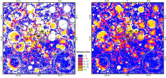
Figure 6. Distance between potential landing sites and water-bearing PSRs in the south polar region (75°–90°S). These distances are calculated from potential landing sites identified in Figure 5 and water-bearing PSRs (black outline), based on slope constraints. Left: distance calculated while traveling on slopes shallower than 10°. Right: distance calculated while traveling on slopes shallower than 15°. The black outlines represent water-ice-bearing PSRs. White pixels represent areas that are not accessible based on the slope constraints (i.e., no distance was calculated).
Download figure:
Standard image High-resolution image4.5. Surface Mobility
We investigated the surface mobility between potential landing sites (illuminated at least 45% of the time on slopes shallower than 5°) and the 169 water-ice-bearing PSRs (Figure 6). We find that six PSRs are accessible (not necessarily their M3 water ice detections) while traversing slopes shallower than 5° only. The minimum distance traveled to access these PSRs varies between ∼2 and 15 km. These PSRs each contain only one water ice detection, except for the PSR located ∼15 km from the landing site, which contains four (PSR 140). If roving on slopes shallower than 10° is allowed, 133 PSRs are accessible. The minimum distance traveled to access these PSRs varies between ∼1 and 95 km. Thus, roving on slopes shallower than 10° allows us to access most water-ice-bearing PSRs, but the distances traveled can be quite long. All, however, are within the 100 km radial distance of an exploration zone as defined by NASA (2015). If roving on slopes up to 15° is allowed, 161 PSRs are accessible. The minimum distance traveled to access these PSRs varies between ∼0.6 and 54 km. Thus, if roving on slopes up to 15° is possible, then almost all PSRs can be accessed and traverse distances become considerably shorter than on 10° slopes. If roving on slopes up to 20° is allowed, 168 PSRs are accessible (i.e., all PSRs except the floor of Shackleton crater). The minimum distance traveled to access these PSRs varies between 0.3 and 42 km. If roving on slopes up to 25° is allowed, 168 PSRs are still accessible (all PSRs except the floor of Shackleton crater). The minimum distance traveled to access these PSRs varies between 0.3 and 41 km. The minimum distance traveled on slopes up to 25° decreases on average by 686 m compared to distances traveled on slopes shallower than 20°. Generally, the capacity to travel on 15° slopes is the best compromise to maximize the number of accessible PSRs and minimize the distance traveled. There appears to be no significant advantage on roving on slopes ≥20°, besides, perhaps, visiting individual water-ice-bearing outcrops.
In Section 4.3.3, we characterized the mobility between the "sunlit" region (or non-PSR region) outside the PSR and at least one M3 detection inside the PSR. We found that at least one M3 detection could be visited while navigating on slopes shallower than 5° from outside of the PSR to inside for Sverdrup 1, Malapert, and Wiechert J. If we now consider a landing site illuminated at least 45% of the time on slope shallower than 5°, the Sverdrup 1 and Malapert PSRs are accessible while navigating on slopes shallower than 10°, while the Wiechert J PSR is accessible while navigating on slopes shallower than 15°. This is because the illumination conditions used herein would not allow landing on the bottom of the given craters.
4.6. Framework for a Coordinated Exploration Effort
In this section we aim to provide a framework for a coordinated exploration effort. As our results have shown, there are a wide variety of water-ice-bearing PSRs. These PSRs contain different properties in terms of hydrogen abundance, WEH, temperature regimes, slope, and illumination conditions. Thus, while different missions will have different scientific and exploration goals, as well as different engineering capabilities, the database of water-ice-bearing PSRs can serve as a guide in planning such missions. To illustrate the types of trades that can be made when selecting a mission profile, here we provide a few examples of site selections that address different mission goals constrained by different scientific objectives and engineering limits.
4.6.1. Sites That Would Allow Sampling the Highest Concentration of Volatiles
To identify sites that provide opportunities to sample the highest concentration of volatiles, we sorted sites in terms of hydrogen abundance as a proxy for water ice and other volatiles within the database. We selected the PSRs that contain on average more than 150 ppm of hydrogen. This results in 21 PSRs, all located on the near side (Table 1). It should be noted that Li et al. (2018) report no bias in the distribution of surficial water ice detections between the near side and far side. Cabeus 1 is the PSR that contains the highest hydrogen abundances and the highest WEH (0.90 wt%) and includes the location of the LCROSS impact site. Cabeus 1 also contains nine surficial water ice detections, which minimizes the chance of visiting a false-positive detection. Other PSRs in Cabeus crater (Cabeus sites 3, 4, and 6) also contain more than 150 ppm of hydrogen and could potentially be visited during the same mission or as part of a coordinated multimission effort. To maximize the chances of success of a given mission, one could instead visit other PSRs that contain the greatest number of surficial ice detections: Shoemaker (134 detections) and Faustini (34 detections). In an initial phase of exploration, one can set aside hydrogen-rich sites that contain less than five surficial water ice detections as primary target locations. However, these sites could be visited as a secondary mission objective.
Table 1. Sites That May Provide Access to the Samples with the Highest Water Ice Abundances
| ID | Name | Latitude (deg) | Longitude (deg) | M3 Detections | Slope (deg) | Hydrogen | Temperature (K) | ||||||
|---|---|---|---|---|---|---|---|---|---|---|---|---|---|
| Counts | Counts km−2 | Max | Mean | Access | Mean (ppm) | Max WEH (wt%) | Min | Max | Mean | ||||
| 37 | Cabeus 1 | −84.4630 | −46.2819 | 9 | 0.03 | 23 | 10 | 5–10 | 171 | 0.90 | 24 | 243 | 51 |
| 87 | −87.8363 | 71.2220 | 1 | 0.80 | 18 | 13 | 15–20 | 168 | 0.11 | 29 | 213 | 52 | |
| 69 | −87.0522 | 55.1529 | 1 | 1.21 | 14 | 5 | 5–10 | 166 | 0.14 | 30 | 111 | 46 | |
| 29 | Cabeus 6 | −83.9778 | −39.3304 | 1 | 5.15 | 15 | 11 | 15–20 | 164 | 0.13 | 42 | 120 | 66 |
| 31 | Cabeus 4 | −84.6090 | −36.7282 | 3 | 0.08 | 24 | 11 | 5–10 | 164 | 0.41 | 29 | 166 | 55 |
| 0 | −87.0182 | 34.5081 | 1 | 25.36 | 10 | 8 | 5–10 | 160 | 0.14 | 29 | 201 | 54 | |
| 2 | −87.0402 | 34.4292 | 1 | 25.36 | 9 | 8 | 5–10 | 160 | 0.14 | 28 | 179 | 53 | |
| 60 | −87.1276 | 40.7185 | 1 | 0.03 | 29 | 21 | 20–25 | 160 | 0.14 | 25 | 220 | 47 | |
| 64 | −86.7877 | 53.6756 | 2 | 0.18 | 22 | 14 | 10–15 | 160 | 0.14 | 36 | 145 | 58 | |
| 65 | −87.0377 | 52.7505 | 1 | 0.37 | 13 | 9 | 10–15 | 160 | 0.14 | 28 | 153 | 46 | |
| 53 | −86.9776 | 32.5309 | 3 | 0.36 | 25 | 18 | 15–20 | 160 | 0.14 | 14 | 106 | 40 | |
| 99 | −88.0593 | 89.0393 | 2 | 0.61 | 26 | 20 | 20–25 | 159 | 0.11 | 32 | 205 | 61 | |
| 70 | −86.7949 | 60.9391 | 3 | 0.13 | 32 | 22 | 15–20 | 158 | 0.14 | 29 | 212 | 48 | |
| 76 | −86.6214 | 68.0028 | 1 | 0.14 | 15 | 8 | 0–5 | 158 | 0.13 | 32 | 162 | 51 | |
| 85 | Shoemaker | −88.0517 | 45.4880 | 134 | 0.13 | 28 | 9 | 10–15 | 157 | 0.24 | 2 | 109 | 44 |
| 38 | Cabeus 3 | −85.3607 | −42.2199 | 1 | 0.03 | 27 | 13 | 10–15 | 156 | 0.60 | 25 | 176 | 58 |
| 102 | Faustini | −87.1557 | 84.0797 | 34 | 0.05 | 30 | 11 | 10–15 | 154 | 0.37 | 14 | 201 | 47 |
| 28 | −84.5571 | 30.2439 | 1 | 1.07 | 15 | 7 | 5–10 | 154 | 0.11 | 42 | 214 | 75 | |
| 98 | −89.2155 | 73.3287 | 2 | 0.30 | 24 | 12 | 10–15 | 152 | 0.10 | 34 | 217 | 64 | |
| 58 | Nobile 4 | −86.3591 | 48.8306 | 6 | 0.05 | 33 | 24 | 20–25 | 152 | 0.28 | 42 | 217 | 74 |
| 95 | −86.3257 | 84.6736 | 1 | 1.91 | 17 | 10 | 0–5 | 151 | 0.08 | 42 | 182 | 71 | |
Note. These 21 PSRs contain on average more than 150 ppm hydrogen (here sorted by mean hydrogen content). These sites are all located on the near side (within ±90° of longitude).
Download table as: ASCIITypeset image
4.6.2. Sites for Characterizing the Lateral Distribution of Water Ice
Determining the compositional distribution (lateral and depth) of the volatile component in lunar polar regions is one of the high-priority goals in lunar science (NRC 2007). The NRC (2007) report articulates the need to study the transport and depositional processes involved in volatile deposits, which, if known, would provide a better model for predicting the sizes of resource reservoirs. To identify sites that may best characterize the lateral distribution of water ice, we identified the PSRs that contain the highest number of surficial water ice detections by M3 (Li et al. 2018). We constrained our analysis on sites that contain at least 10 surficial water ice detections, plus Cabeus 1 with nine detections. These represent 13 PSRs, including nine PSRs on the near side (Table 2). Three PSRs contain the highest number of detections: Shoemaker (134), Sverdrup 1 (93), and Haworth (80). Sverdrup 1 appears particularly interesting, as its slopes are shallower than Shoemaker and Haworth. The remaining 10 PSRs also appear to be good candidates, except for Shackleton, for which the water ice detections are located on the walls of the crater, which consist of slopes steeper than 25°.
Table 2. Sites That Would Allow Us to Best Characterize the Lateral Distribution of Water Ice
| ID | Name | Latitude (deg) | Longitude (deg) | M3 Detections | Slope (deg) | Hydrogen | Temperature (K) | ||||||
|---|---|---|---|---|---|---|---|---|---|---|---|---|---|
| Counts | Counts km−2 | Max | Mean | Access | Max (ppm) | Max WEH (wt%) | Min | Max | Mean | ||||
| 85 | Shoemaker | −88.0517 | 45.4880 | 134 | 0.13 | 28 | 9 | 10–15 | 168 | 0.24 | 2 | 109 | 44 |
| 127 | Sverdrup 1 | −88.2432 | −143.9156 | 93 | 0.17 | 26 | 7 | 0–5 | 141 | 0.12 | 28 | 125 | 55 |
| 62 | Haworth | −87.5109 | −2.2324 | 80 | 0.08 | 31 | 9 | 5–10 | 145 | 0.31 | 14 | 128 | 42 |
| 120 | −88.7290 | 168.8992 | 36 | 0.41 | 22 | 6 | 5–10 | 141 | 0.15 | 28 | 174 | 47 | |
| 102 | Faustini | −87.1557 | 84.0797 | 34 | 0.05 | 30 | 11 | 10–15 | 168 | 0.37 | 14 | 201 | 47 |
| 108 | Shackleton | −89.6782 | 126.8822 | 34 | 0.15 | 35 | 27 | 25+ | 152 | 0.17 | 20 | 173 | 63 |
| 154 | Wiechert J | −85.0288 | −140.3766 | 17 | 0.05 | 30 | 12 | 0–5 | 94 | 0.06 | 36 | 180 | 66 |
| 25 | Malapert | −84.1452 | 5.9438 | 17 | 0.09 | 33 | 15 | 0–5 | 97 | 0.05 | 37 | 206 | 66 |
| 54 | Nobile 2 | −84.5522 | 60.2933 | 15 | 0.08 | 24 | 9 | 0–5 | 121 | 0.13 | 31 | 137 | 57 |
| 89 | −88.9996 | −42.9735 | 10 | 0.24 | 17 | 5 | 0–5 | 140 | 0.84 | 33 | 123 | 53 | |
| 57 | −87.3678 | −30.7628 | 10 | 0.31 | 25 | 11 | 5–10 | 135 | 0.08 | 27 | 96 | 47 | |
| 42 | Nobile 3 | −84.2905 | 56.3477 | 10 | 0.10 | 34 | 23 | 20–25 | 120 | 0.12 | 39 | 250 | 64 |
| 37 | Cabeus 1 | −84.4630 | −46.2819 | 9 | 0.03 | 23 | 10 | 5–10 | 178 | 0.90 | 24 | 243 | 51 |
Note. These best sites are PSRs for which the highest number of M3 detections have been found. Here we show the characteristic of 12 PSRs for which at least 10 water ice detections have been reported and one PSR in Cabeus crater (Cabeus 1) for which nine detections have been reported. PSRs are sorted by their number of M3 detections of water ice. Sites within ±90° of longitude are located on the near side. Shackleton appears in italics, as accessing the M3 detections would require to navigate on slopes steeper than 25°.
Download table as: ASCIITypeset image
4.6.3. Sites for Characterizing the Vertical Distribution of Volatiles
The surficial detections of water ice by M3 are limited to the uppermost surface. However, to determine the resource potential of an area for a sustainable exploration program and to determine whether there is a stratigraphy of volatiles that can be used to address science objectives, it is necessary to evaluate the distribution of volatiles as a function of depth in the regolith. To identify sites that provide the best opportunities to characterize the vertical distribution of volatiles, we identified the PSRs for which water ice and dry ice may be thermally stable within the top meter of the regolith. We searched for the PSRs for which the maximum depth of stability of water ice is smaller than 1 m (implying that anywhere in a given PSR water ice could be present somewhere between the surface and 1 m below) and the minimum depth of stability of dry ice is also smaller than 1 m (implying that somewhere in a given PSR dry ice should be present in the top meter).
We find that 76 PSRs meet these criteria (Figure 3, Table 3). However, in most of these PSRs, only one M3 surficial detection has been reported. Thus, to maximize the chances of successfully finding surficial detections in situ, we identify 11 sites that contain at least 10 surficial water ice detections, including Cabeus 1 (nine detections), which could be used to validate LCROSS measurements. Within these 11 PSRs (Table 3), water ice becomes stable between the surface and a maximum of 43 cm deep. Dry ice becomes stable either at the surface or at a depth of ∼10 cm. Thus, if present in the subsurface, water ice and dry ice may be accessible by shallow trenching or using a 1 m drill.
Table 3. Sites That Allow Us to Best Characterize the Vertical Distribution of Volatiles
| ID | Name | Latitude (deg) | Longitude (deg) | M3 Detections | H2O Depth (m) | CO2 Depth (m) | |||
|---|---|---|---|---|---|---|---|---|---|
| Counts | Counts km−2 | Min | Max | Min | Max | ||||
| 85 | Shoemaker | −88.0517 | 45.4880 | 134 | 0.24 | 0.00 | 0.11 | 0.00 | 2.50 |
| 127 | Sverdrup 1 | −88.2432 | −143.9156 | 93 | 0.12 | 0.00 | 0.32 | 0.00 | 2.50 |
| 62 | Haworth | −87.5109 | −2.2324 | 80 | 0.31 | 0.00 | 0.36 | 0.00 | 2.50 |
| 120 | −88.7290 | 168.8992 | 36 | 0.15 | 0.00 | 0.25 | 0.09 | 2.50 | |
| 102 | Faustini | −87.1557 | 84.0797 | 34 | 0.37 | 0.00 | 0.43 | 0.00 | 2.50 |
| 25 | Malapert | −84.1452 | 5.9438 | 17 | 0.17 | 0.00 | 0.24 | 0.00 | 2.50 |
| 154 | Wiechert J | −85.0288 | −140.3766 | 17 | 0.06 | 0.00 | 0.31 | 0.00 | 2.50 |
| 54 | Nobile 2 | −84.5522 | 60.2933 | 15 | 0.05 | 0.00 | 0.18 | 0.00 | 2.50 |
| 57 | −87.3678 | −30.7628 | 10 | 0.13 | 0.00 | 0.15 | 0.00 | 2.50 | |
| 89 | −88.9996 | −42.9735 | 10 | 0.84 | 0.00 | 0.14 | 0.12 | 2.50 | |
| 37 | Cabeus 1 | −84.4630 | −46.2819 | 9 | 0.08 | 0.00 | 0.11 | 0.00 | 2.50 |
Download table as: ASCIITypeset image
4.6.4. Sites That Would Allow the Fastest Recovery of a Scientifically Interesting Sample
To identify sites that would allow the fastest recovery of a scientifically interesting sample, we evaluated the distance from potential landing sites to PSR boundaries. We classified the PSRs from the shortest distance to be traveled between the landing site and the PSR boundary while navigating on slopes shallower than 5°, then 10°, 15°, 20°, and 25°. We excluded PSRs that would require navigating more than 10 km in all slope ranges, PSRs containing five or fewer surficial water ice detections, and PSRs for which the water ice detections are located on slopes steeper than 20°.
This resulted in the identification of 14 PSRs (Table 4), including Nobile 2, Malapert crater, Sverdrup 1, Faustini, Wiechert J, Shoemaker, and several unnamed PSRs. Accessing these PSRs requires navigating on slopes steeper than 5°, and thus no distance to a PSR is reported for the 0°–5° slope range. A Nobile 2 site appears to be the most promising location, because it is within ∼4 km of a landing site with access across 0°–10° slopes (or within ∼2 km if a portion of the traverse can accommodate 15° slopes) and 15 water ice detections. It also contains favorable illumination conditions with an average illumination of 45% within 1 km of the PSR boundary and 54% within 5 km (Euclidian distance) of the PSR boundary. Seven other PSRs are accessible while navigating on 0°–10° slopes, including Malapert and Sverdrup 1. Sverdrup 1 contains the most favorable illumination conditions of the 14 PSRs, with average illumination reaching 77% of the time, within 10 km of the PSR boundary. Faustini, Wiechert J, and Shoemaker craters and PSR 120 are accessible when navigating on 0°–15° slopes. However, their distance to the closest landing site is under 10 km only when navigating on 0°–20° slopes occasionally.
Table 4. PSRs That Are Located the Closest to Potential Landing Sites While Navigating on Different Slopes Ranges and for Which More Than Five Surficial Water Ice Detections Have Been Reported
| ID | Name | Latitude (deg) | Longitude (deg) | M3 Detections | Minimum Distance to PSR (m) | Illumination (%) | ||||||
|---|---|---|---|---|---|---|---|---|---|---|---|---|
| Counts | Counts km−2 | 10° | 15° | 20° | 25° | 1 km | 5 km | 10 km | ||||
| 54 | Nobile 2 | −84.5522 | 60.2933 | 15 | 0.08 | 3836 | 2028 | 2028 | 2028 | 45 | 54 | 54 |
| 123 | −88.3241 | 147.4953 | 6 | 0.12 | 5326 | 3509 | 2326 | 2326 | 10 | 71 | 71 | |
| 57 | −87.3678 | −30.7628 | 10 | 0.31 | 7549 | 7479 | 7467 | 7467 | 9 | 37 | 62 | |
| 101 | −84.1835 | −88.9602 | 6 | 0.10 | 15,243 | 8323 | 8323 | 8323 | 23 | 44 | 47 | |
| 25 | Malapert | −84.1452 | 5.9438 | 17 | 0.09 | 15,413 | 9792 | 5906 | 1800 | 43 | 55 | 55 |
| 120 | −88.7290 | 168.8992 | 36 | 0.41 | 16,356 | 10,400 | 6601 | 6391 | 6 | 44 | 64 | |
| 127 | Sverdrup 1 | −88.2432 | −143.9156 | 93 | 0.17 | 20,741 | 8583 | 4527 | 3684 | 29 | 55 | 77 |
| 84 | −89.0405 | −22.2154 | 9 | 0.16 | 23,192 | 7222 | 6180 | 6180 | 13 | 45 | 45 | |
| 15 | −82.1734 | 11.1022 | 8 | 0.03 | 1618 | 869 | 869 | 47 | 54 | 55 | ||
| 26 | −84.2441 | −13.1782 | 7 | 0.17 | 4106 | 3319 | 3240 | 35 | 46 | 46 | ||
| 78 | −88.7248 | −13.7107 | 6 | 0.11 | 6824 | 5276 | 3725 | 12 | 45 | 52 | ||
| 102 | Faustini | −87.1557 | 84.0797 | 34 | 0.05 | 10,433 | 4784 | 4243 | 5 | 65 | 68 | |
| 154 | Wiechert J | −85.0288 | −140.3766 | 17 | 0.05 | 11,204 | 7548 | 6720 | 41 | 45 | 50 | |
| 85 | Shoemaker | −88.0517 | 45.4880 | 134 | 0.13 | 13,843 | 9134 | 8160 | 2 | 24 | 47 | |
Download table as: ASCIITypeset image
4.6.5. Summary of Site Assessments
We identified 36 water-ice-bearing PSRs (all PSRs shown in tables excluding Shackleton) with the highest hydrogen abundances that allow us to best characterize the lateral distribution of water ice, that allow us to best characterize the vertical distribution of water ice, or that allow the fastest recovery of a scientifically interesting sample. To maximize the scientific results from upcoming missions, sites that would allow us to fulfill more than one science objective should be visited in priority. Eleven PSRs should allow this endeavor and are presented in Figure 8 and Table 5. These PSRs are Shoemaker, Faustini, Cabeus 1, Malapert, Nobile 2, Sverdrup 1, Wiechert J, Haworth, and unnamed PSRs 57, 120, and 89. These sites are located within 6° of the pole and could thus constitute regions of interest for the Artemis III program.

Figure 8. The 11 water-ice-bearing south polar PSRs that would allow us to study more than one of the following objectives: the highest hydrogen abundances, the lateral distribution of water ice, the vertical distribution of volatiles, or the fastest recovery of a scientifically interesting sample. Sites in dark green allow us to study all four objectives, in medium green three objectives, and in light green two objectives. All sites are located within 6° of the south pole, in line with the Artemis III landing area. The LOLA DEM is shown as a base map.
Download figure:
Standard image High-resolution imageTable 5. The 11 PSRs That Would Allow Us to Fulfill More Than One Science Objective Should and Are Thus Considered as High-priority Targets
| ID | Name | Latitude (deg) | Longitude (deg) | Area (km2) | M3 Detections | Science Objective | Age (Ga) | ||||
|---|---|---|---|---|---|---|---|---|---|---|---|
| Counts | Counts km−2 | Highest Abun. | Lateral Dist. | Vertical Dist. | Fastest Sample | ||||||
| 85 | Shoemaker | −880,517 | 454,880 | 1071 | 134 | 0.13 | X | X | X | X | 4.15 |
| 102 | Faustini | −871,557 | 840,797 | 660 | 34 | 0.05 | X | X | X | X | 4.10 |
| 25 | Malapert | −841,452 | 59,438 | 191 | 17 | 0.09 | X | X | X | ⋯ | |
| 37 | Cabeus 1 | −844,630 | −462,819 | 285 | 9 | 0.03 | X | X | X | 3.50 | |
| 54 | Nobile 2 | −845,522 | 602,933 | 178 | 15 | 0.08 | X | X | X | 3.80 | |
| 57 | −873,678 | −307,628 | 32 | 10 | 0.31 | X | X | X | ⋯ | ||
| 120 | −887,290 | 1,688,992 | 87 | 36 | 0.41 | X | X | X | ⋯ | ||
| 127 | Sverdrup 1 | −-882,432 | −1439,156 | 541 | 93 | 0.17 | X | X | X | 3.80 | |
| 154 | Wiechert J | −850,288 | −1,403,766 | 367 | 17 | 0.05 | X | X | X | 3.20 | |
| 62 | Haworth | −875,109 | −22,324 | 1009 | 80 | 0.08 | X | X | 4.18 | ||
| 89 | −889,996 | −429,735 | 42 | 10 | 0.24 | X | X | ⋯ | |||
Note. The absolute model age for some of these PSRs is also given (Deutsch et al. 2020).
Download table as: ASCIITypeset image
4.6.6. Potential Volatile Sources and ISRU Considerations for High-priority PSRs
The absolute model age for 20 large (count areas ≥100 km2) south polar (80°–90°S) craters that host surface ice has been calculated by Deutsch et al. (2020), which can provide information regarding the potential sources of the volatiles expected to be present at those sites. In sites older than 3.8 Ga (e.g., Nobile 2, Sverdrup 1, Faustini, Shoemaker, Haworth), volatiles may have been derived from impacting asteroids, comets, impact-generated degassing of the Moon, and volcanic degassing of the mantle. Sites with ages between ∼3 and ∼3.8 Ga (e.g., Wiechert J, Cabeus 1) may have trapped volatiles released mostly by volcanism, sporadic impact events, and the ever-present solar wind and micrometeoritic impacts. Volatile deposits on the floors of those craters could have been modified by ballistic sedimentation of ejecta from nearby craters and buried by that ejecta (Kring 2020). The age of the PSR in Malapert crater, as well as unnamed PSRs 57, 120, and 89, was not calculated, and thus their potential sources of volatiles are unknown.
The potential sources of the volatiles expected to be present at those sites are, however, likely different in the uppermost meter of the surface (where most science and ISRU missions will have access) than at greater depths. Nominally, sites within the 11 identified PSRs of interest would have accumulated ∼3–4 m of regolith using a typical regolith production rate of 1 m per billion years (Hörz et al. 1991). Model calculations suggest that small impact cratering events would have episodically buried volatiles that accumulate through the surface, producing multiple horizons of ice within those 4 m of regolith (e.g., Figure 5 of Crider & Vondrak 2003). However, as the distinct ages of craters in Table 5 imply, significant amounts of impact ejecta were also being distributed throughout the region. For example, in Shoemaker crater (Figure 8), ejecta layers from Faustini, Amundsen, and Nobile were , and m thick, respectively (Kring et al. 2020a, 2020b). Thus, if ice accumulated in the ∼50-, ∼200-, and ∼100-million-year intervals between those impacts, it may have been buried beneath that ejecta, far below the 1–4 m of regolith easily accessible at the surface. Moreover, the ejecta landed with velocities of order 100 and 1000 km hr−1 (Kring 2020), which may have severely modified the distribution of any ices in the regolith being buried. It thus seems reasonable to anticipate that the volatiles detected at the surface from orbit were deposited after the last major impact event to blanket each of the 11 sites identified here. Although impact cratering during the basin-forming epoch may have dominated the flux of volatiles delivered to the lunar surface (Lucey et al. 2020), those impact events may not have dominated material in the uppermost meters of the sites in Figure 8. Instead, their surfaces may have accumulated volatiles from sporadic impact events, volcanically vented gases (Kring 2014; Kring et al. 2014; Needham & Kring 2017; Wilson et al. 2019), crustal degassing (Taylor et al. 2018), micrometeorites (Hurley et al. 2017), and solar wind (Hurley et al. 2017). For example, in Faustini, after Nobile and potentially Imbrium, Schrödinger, and Orientale ejecta landed at ∼3.8 Ga, the regolith may have accumulated volatiles from circa 3.5 Ga volcanism, sporadic impacts, micrometeorites, and the solar wind. If accumulation in the regolith only occurred within the past 2 Ga (Siegler et al. 2016), after a shift in the polar axis (Siegler et al. 2016), the volatiles within the site identified here may be dominated by sporadic impacts, such as those that may have occurred in pulses 800 (Kring et al. 1996; Kring 2007, 2008; Terada et al. 2020) and 470 Ma (Schmitz et al. 2001; Swindle et al. 2014), micrometeorites, and solar wind. If the uppermost meter of regolith in the 11 sites only caries a volatile signature from the last billion years, then it may be dominated by micrometeorites and solar wind.


The size of the 11 high-priority PSRs can be used to estimate the amount of water ice present and thus inform ISRU possibilities. The PSRs in Haworth (1009 km2), Shoemaker (1071 km2), and Faustini (660 km2) craters are the largest among the high-priority PSRs. If water ice exists in the thermal stability zone described in Section 3.2 for these craters, then the PSRs in Haworth and Shoemaker may each have 9 × 10⁹–3 × 10¹⁰ kg of water ice, while the PSR in Faustini may have 6 × 10⁹–2 × 10¹⁰ kg of water ice, assuming that 5.6 ± 2.9 wt% H2O is present in the regolith, as determined from the LCROSS experiment (Kring et al. 2020a, 2020b). These are upper limit values, because thermal stability does not ensure deposition, nor preservation against other processes such as impact gardening. The Sverdrup 1 PSR (541 km2) would have a similar amount of water ice, although somewhat smaller than the PSR in Faustini.
For ISRU purposes, an annual production rate of 10 metric tons or 15 metric tons of H2O has been suggested for NASA planning purposes (G. Sanders 2020, personal communication). At that rate, a 600,000–2,000,000 yr supply might exist within the uppermost meter of Haworth and Shoemaker craters' regolith. In another study (Kornuta et al. 2019), an annual production demand of 2450 metric tons of lunar water is anticipated. At that rate, Haworth crater may have a 3600 yr supply. Thus, validating the surface detection of water ice and evaluating the horizontal and vertical distribution of any ice will be important for a sustainable exploration program that utilizes in situ resources.
4.6.7. Notable Exceptions
There are two notable exceptions of craters that have been previously identified as potential sites to study volatiles that are not being proposed here, Shackleton and Amundsen. As mentioned above, the analysis of M3 data suggests that the walls of Shackleton crater contain water ice. However, these walls are steep (>25°), and thus we do not recommend visiting the site, mostly based on mobility difficulties. However, even if mobility was not an issue, visiting Shackleton would only allow us to study one of the four potential science objectives described herein (the lateral distribution of volatiles) and thus does not appear as one of the most promising sites. Amundsen crater has also been suggested as a potentially interesting site to study polar volatiles (e.g., Lemelin et al. 2014; Flahaut et al. 2020), as they may be stable in a large PSR on the floor of the crater. However, it was excluded from our analysis owing to the lack of surficial water ice detection by M3. Amundsen crater is an appealing target (it has a broad flat floor, a central peak, and favorable illumination conditions and temperature regime), as it provides an opportunity to conduct telerobotic subsurface surveys of water and dry ice across thermal gradients (Kring 2017; Allender et al. 2019) in areas where it should exist in the upper meter of regolith (Kring et al. 2020a, 2020b) and has geologic targets that address a large number of other NRC (2007) science objectives (Lemelin et al. 2014).
5. Case Studies
We chose 3 of the 11 most promising sites to study polar volatiles and present case studies in them with three different traverse lengths: a relatively short distance mission (20–50 km) to PSR 89, a medium-length mission (∼100 km) to Sverdrup 1, and a longer distance mission (∼300 km) to Cabeus crater. For each of these sites, we identified the landing site as one of the 50 most often illuminated places calculated by Mazarico et al. (2011) and identified alternative landing sites in some cases that could shorten the mission. For each of these landing sites, we calculated the maximum and average number of days of uninterrupted and interrupted Sun periods between 2030 and 2023 January 1 using a 120 m pixel–1 LOLA DEM (Table 6). We then calculated the "cost" of traveling from the given landing site to surficial water ice detections in each PSR. A cost raster was established using slope (here at 30 m pixel–1) and illumination as constraints. Mobility was allowed on slopes <15° only. The slope values (0°–15°) were reclassified into values ranging between 0 (low cost for shallow slopes) and 10 (high cost for steeper slopes). The illumination data set (0%–100%) was also reclassified into values ranging between 0 (low cost for high illumination) and 10 (high cost for low illumination). These two reclassified data sets were then added and weighted equally to create a cost raster. We calculated the least cost path (including the cost distance and the cost backlink) between each landing site and selected sampling sites (surficial M3 detections) to derive potential traverses.
Table 6. Illumination Conditions for the Potential Landing Sites Identified in the Three Case Studies Using a 120 m pixel–1 LOLA DEM and the Method of Mazarico et al. (2011) for the Period between 2030 and 2023 January 1
| Landing Site | Maximum (days) | Average (days) | ||||
|---|---|---|---|---|---|---|
| Uninterrupted Sun | Interrupted Sun | Uninterrupted Night | Uninterrupted Sun per Month | Interrupted Sun per Month | Uninterrupted Night per Month | |
| PSR 89 | ||||||
| 016 | 175.04 | 203.08 | 12.58 | 27.15 | 27.75 | 8.36 |
| A | 19.75 | 19.75 | 23.08 | 17.33 | 18.38 | 18.18 |
| Sverdrup 1 | ||||||
| 004 | 176.58 | 292.83 | 5.50 | 31.69 | 34.13 | 3.83 |
| A | 19.42 | 19.42 | 17.04 | 17.32 | 18.57 | 18.19 |
| B | 21.42 | 21.42 | 14.21 | 22.19 | 22.50 | 13.32 |
| C | 13.62 | 13.62 | 23.25 | 11.23 | 11.50 | 24.28 |
| Cabeus | ||||||
| 030 | 117.00 | 174.50 | 11.29 | 29.22 | 29.75 | 6.29 |
Download table as: ASCIITypeset image
5.1. A Short-distance Mission to PSR 89
PSR 89 was identified as one of the sites that provides a good opportunity to characterize the lateral (it contains 10 water ice detections) and vertical distribution of volatiles (both water ice and dry ice, if present, would be thermally stable in the top meter of the regolith). It contains elevated hydrogen abundances, with an average value of 140 ppm. Its temperature regime is cold, with a minimum annual temperature of 33 K, a maximum annual temperature of 123 K, and an average annual temperature of 53 K. Here we present two potential traverses to this PSR, a ∼50 km traverse that lands at one of the 50 most illuminated places in the south polar region (Mazarico et al. 2011), and a ∼20 km traverse that lands at one of the potential landing sites identified in Section 4.4 (Figure 9). This mission would operate on the near side of the Moon.

Figure 9. Potential traverses across water-ice-bearing PSR 89. A ∼50 km traverse (solid line) could land at site 016 of Mazarico et al. (2011) (8868S, 6842W) and sample multiple water ice detections inside and outside PSRs 89 and 90. Alternatively, a ∼20 km traverse (dashed line) would land at site A (8852S, 4912W) and sample multiple water ice detections inside and outside PSRs 80 and 89. The stars represent M3 detections of surficial water ice, and the polygons represent water-ice-bearing PSRs (PSRs 89, 26, and 24 are part of the 40 most promising PSRs).
Download figure:
Standard image High-resolution imageThe ∼50 km traverse would land at site 016, at 8868S, 6842W, on the rim of de Gerlache crater. This site is illuminated on average 83% of the time and is located on the near side of the Moon. The traverse would then go toward PSR 89, sampling surficial water ice detection 348 on the way (traveling length of 20,473 m). This represents an interesting opportunity to sample a water ice detection that is not collocated with the PSR polygons used herein and could thus inform on the potential presence of water ice in PSRs smaller than 240 m or on transient water ice deposits. The traverse would then enter the PSR and sample sites 343 (3679 m) and 398 (4316 m). It would exit the PSR and sample site 401 (4899 m), another water ice detection outside the PSR. Two other water ice detections (399 and 400) could be sampled along the way, between sites 398 and 401. Ice detection 400 is located inside a small PSR (PSR 90). If ended here, the traverse length would be 33,367 m. Different options are available after sampling site 401. Here we suggest returning to the landing site, for a total traverse length of 55,239 m. Alternatively, nearby PSRs 75, 80, 84, or 94 could be visited, as their surface slopes are also shallower than 15°. Such a traverse could be accomplished by a Lunar Prospecting Rover (LPR) class rover. This (canceled) rover designed by ESA had mission requirements consisting of a mobile range of 50 km, an average illumination fraction >0.25, and Earth visibility for direct-to-Earth communication (e.g., Carpenter et al. 2015; Flahaut et al. 2020).
The ∼20 km traverse would land at site A located at 8852S, 4912W (identified in Section 4.4). This site is illuminated on average 47% of the time and is located on the near side of the Moon. The traverse would then go toward PSR 80, sampling ice detection 320 along the way (6646 m) outside the PSR and then sampling detection 321 inside PSR 80 (3120 m). The traverse would then head toward PSR 89, sampling detection 338 (4308 m) before entering the PSR and then sampling detections 363 (3576 m) and 381 (1419 m) both inside the PSR. If ended here, the traverse length would be 19,069 m. Sampling site 381 is located approximately 300 m from the PSR boundary; thus, exiting the PSR would represent a total traverse of ∼20 km. Such a traverse could be accomplished by a VIPER-class rover. That rover has a mobile range of ∼20 km for a 100-Earth-day mission duration (NASA 2020).
5.2. A Medium-length Traverse Mission to Sverdrup 1
Sverdrup 1 was identified as one of the sites that provides an opportunity to characterize the lateral (it contains 93 water ice detections) and vertical (both water ice and dry ice should be thermally stable within the top meter of the regolith) distribution of volatiles. It was also identified as one of the sites that would allow the fastest recovery of a scientifically interesting sample, as it is located less than 10 km away from a potential landing site (illuminated at least 45% of the time with slopes shallower than 5°) while navigating on slopes shallower than 15°. It contains enhanced hydrogen abundances, with an average value of 104 ppm. Its temperature regime is cold, with a minimum annual temperature of 32 K, a maximum annual temperature of 187 K, and an average annual temperature of 55 K. Sverdrup crater is 3.8 Ga (Deutsch et al. 2020). Here we present one potential traverse to this PSR, a ∼90 km traverse that lands at one of the 50 most illuminated places in the south polar region (Mazarico et al. 2011) on the rim of Shackleton crater, and also propose alternative landing sites that could shorten the mission (Figure 10). This mission would operate on the far side of the Moon.

Figure 10. Potential traverse across the water-ice-bearing Sverdrup 1 PSR. The landing site could take place at site 004 (8978S, 15573W; Mazarico et al. 2011) and sample multiple water ice detections from M3. Left: slope. Right: illumination conditions. The stars represent M3 detections of surficial water ice, the polygons represent water-ice-bearing PSRs (Sverdrup 1 and PSR 120 are part of the 40 most promising PSRs), and the bold black line represents a potential traverse. The landing site for a short-duration mission to PSR 89 is also shown (Site 016).
Download figure:
Standard image High-resolution imageA ∼90 km traverse would begin at landing site 004 (8978S, 15573W; Mazarico et al. 2011), on the rim of Shackleton crater. This site is illuminated on average 87% of the time. The traverse would then analyze a scientifically interesting sample at our site 510 (7403 m), in water-ice-bearing PSR 107. The traverse would then head toward Sverdrup crater, to site 315 (34,306 m), another small PSR (PSR 115). The traverse would then enter the Sverdrup 1 PSR and head toward to the coldest area (avg. T = 44 K) at site 228 (10,493 m). The traverse would then head toward site 335 (13,263 m) on the edge of the Sverdrup 1 PSR. It could then follow the edge of the PSR and sample 13 surficial ice detections until reaching point 432 to exit the PSR (15,598 m). The traverse would then climb outside of Sverdrup crater and sample a final water ice detection at site 503 (11,191 m). This traverse would have a length of 92,254 m. From this point, the traverse could go to a topographically high point on the margin of Sverdrup, sample nearby water-ice-bearing PSRs 120 and 126, or go back to Shackleton crater.
As for the short-duration mission presented in Section 5.1, landing in one of the 50 most illuminated places of the south polar region adds a considerable length to the mission. Landing in a less illuminated region could help shorten the mission, such as landing sites A, B, or C presented in Figure 7. Landing at site C would allow us to keep nearly the same traverse but reverse the sample station order. Landing at site A or B would exclude sampling sites 510 and 315. With either of these options, the length of the traverse could be shortened nearly by half (∼51 km).

Figure 7. Distance between potential landing sites (black pixels) and water-bearing PSRs (black outline) in Sverdrup, Malapert, and Wiechert J craters while navigating on slopes shallower than 15° (Figure 7). White pixels represent areas that are not accessible based on the slope constraint. White stars represent M3 detections of surficial water ice from Li et al. (2018). Three potential landing sites (which minimize the distance traveled) are present around Sverdrup 1 within Sverdrup crater: A (8797S, 11320W) is the closest to a PSR boundary (∼12 km), while B (8781S, 16030W) and C (8770S, 16870W) are farther away (∼14 to 15 km). In Malapert crater, a potential landing site (A) is present ∼10 km from a PSR boundary. In Wiechert J crater, a potential landing site is located ∼13 km from a PSR boundary. Red stars represent the most illuminated places derived by Mazarico et al. (2011).
Download figure:
Standard image High-resolution image5.3. A Long-duration Mission to Cabeus
Cabeus crater (and its different water-ice-bearing PSRs) was identified as the site that would allow sampling the highest concentration of volatiles, with average hydrogen abundances reaching 171 ppm in Cabeus 1. Cabeus crater is 3.5 Ga (Deutsch et al. 2020); it is thus a younger catchment than the Sverdrup catchment. It was also identified as one of the sites that would allow us to best characterize the lateral (Cabeus 1 contains nine water ice detections) and vertical (water ice and dry ice are both stable within the top meter of the regolith in Cabeus 1) distribution of volatiles. The temperature regime in Cabeus 1 is cold, with a minimum annual temperature of 24 K, a maximum annual temperature of 243 K, and an average annual temperature of 51 K. Here we present one potential traverse to this PSR, a ∼300 km traverse that begins at a landing site from among the 50 most illuminated places in the south polar region (Mazarico et al. 2011) on Malapert massif (Figure 11). This mission would operate on the near side of the Moon.

Figure 11. Potential traverse across Cabeus crater. The landing site could take place at site 030 of Mazarico et al. (2011) (8596S, 320W) on Malapert massif and sample multiple water ice detections from M3. Left: slope. Right: illumination conditions. The stars represent M3 detections of surficial water ice, the polygons represent water-ice-bearing PSRs (Cabeus 1–4, Haworth, and PSR 78 are part of the 37 most promising PSRs), the green circle represents the LCROSS impact site, and the bold black line represents a potential traverse.
Download figure:
Standard image High-resolution image
The ∼300 km traverse would land at site 030, at 8596S, 320W, on Malapert massif. This site is illuminated on average 81% of the time and has been suggested as a potential lunar base by Basilevsky et al. (2019). The traverse would travel to PSR 15 and sample site 278 (31,929 m). It would then drive into Cabeus crater, head toward PSR Cabeus 4, and sample sites 88 (71,767 m) and 81 (2967 m). It would then head toward Cabeus 1, sample sites 69 (20,404 m) and 57 (8360 m), and exit the PSR while traveling to site 66 (15,584 m), a water ice detection outside PSRs. The LCROSS impact site is in Cabeus 1, between sites 57 and 66, and would be sampled along the way. The traverse would then head toward Cabeus 3, sampling site 86 (23,252 m) before entering the PSR, then site 90 (4056 m) inside the PSR. The traverse would head outside of Cabeus, to site 300, which is located next to PSR 39 (71,456 m). It would then sample sites 326 (15,548 m) and 322 (9142 m), water ice detections outside PSRs, and travel back to Malapert massif (27,364 m). This traverse would have a length of 301,829 m. As opposed to the previous two potential missions presented, a mission to Cabeus could not be shortened considerably while landing at one of the potential landing sites presented in Section 4.4. The potential landing site located the closest to site 278 is located ∼10 km away, which would reduce the traverse length by ∼20 km each way for a total traverse length of ∼260 km. We note, however, that such a long-duration mission to Cabeus crater could be conducted as a "stand-alone" mission or could be integrated into the traverse proposed by Allender et al. (2019) for the ISECG-GER design reference mission for humans on the lunar surface. A portion of this traverse (near sites 278, 300, 326, and 322) was also previously studied as the "North Haworth" region by Heldmann et al. (2016) for the NASA's Resource Prospector (now VIPER) mission.
6. Conclusion
We conducted a systematic study of the 169 water-ice-bearing PSRs (based on M3 observations) in the south polar region of the Moon to identify promising sites to study volatiles. We built a database of water-ice-bearing PSRs, including information that could be used to help identify the best location for missions designed to validate the detections of water ice at the surface and extend those observations to determine the lateral and vertical extent of that ice, noting that multiple missions are possible and may involve several space agencies and commercial partners. The exploration sites are constrained by surface and subsurface temperatures, slope, hydrogen content, number of water ice detections, thermal stability depths for water ice and dry ice, and mobility range (e.g., distance from potential landing sites to sites of detected water ice). Using this database, we identified 21 sites that provide access to samples with the highest abundance of volatiles, 13 sites that provide the best opportunities to characterize the lateral distribution of volatiles, 11 sites that provide the best opportunities to characterize the vertical distribution of volatiles (water ice and dry ice), and 14 sites that would allow the fastest recovery of a scientifically interesting sample. Together, these sites occur in 37 different water-ice-bearing PSRs. Among them are 11 PSRs that meet more than one of those criteria and may therefore be of particular interest for exploration. These PSRs are Shoemaker, Faustini, Cabeus 1, Malapert, Nobile 2, Sverdrup 1, Wiechert J, Haworth, and unnamed PSRs 57, 120, and 89.
These sites and their characteristics illustrate the trades available between different mission scenarios and illustrate those sites that may warrant a high-resolution (i.e., 0.5 m scale) evaluation of Narrow Angle Camera and Terrain Camera imagery. Potential traverses to 3 of the 11 most promising sites further show the trades available between different mission scenarios. The traverses differ in distance between a landing site and ice-detection site: a 20–50 km traverse to PSR 89, a ∼100 km traverse to Sverdrup 1, and a ∼300 km traverse to Cabeus. In all cases, the landing site occurs in one of the high-illumination points in the south polar region (Mazarico et al. 2011) and provides access to more than one PSR where multiple M3 surficial water ice detections exist.
The database of water-ice-bearing PSRs can be found in Zenodo as an Excel table or an ESRI shapefile (doi:10.5281/zenodo.4646092). The authors would like to thank Richard Elphic and two anonymous reviewers for their comments and suggestions, which greatly improved the quality of the manuscript. The authors would also like to thank Simon Trottier and Geneviève Crevier at the Université de Sherbrooke for their help with the geospatial data analysis, and G. (Jerry) Sanders for information about anticipated ISRU water production rates. This research was undertaken, in part, thanks to funding from the Canada Research Chair in Northern and Planetary Geological Remote Sensing (950-232175) and an NSERC Discovery grant held by Myriam Lemelin. D.A.K. was supported by NASA Solar System Exploration Research Virtual Institute contract 80NSSC20M0016. This is LPI Contribution No. 2608. LPI is operated by USRA under a cooperative agreement with the Science Mission Directorate of the National Aeronautics and Space Administration.