


Abstract
Using the Hubble Space Telescope, Saturn was observed in 2018, 2019, and 2020, just after the northern hemisphere summer solstice. Analysis of multispectral imaging data reveals three years of cloud changes associated with a 70° N storm that began in 2018. Additionally, there is an increase in equatorial brightness and perhaps haze optical depth at 0° to 7° N. There are small midsummer changes at the north pole, with a thin blue feature near the polar hexagon's outer edge disappearing between 2019 and 2020 and increasingly reddish polar haze. Zonal winds at most latitudes remain close to values obtained by the Cassini mission with a slight increase of winds in the equatorial zone. Yearly cloud changes, while noticeable, are small compared with the changes observed between the Voyager (northern spring) and Cassini (southern summer to northern spring) eras, but further observations will provide a longer baseline for comparison.
Export citation and abstract BibTeX RIS

Original content from this work may be used under the terms of the Creative Commons Attribution 4.0 licence. Any further distribution of this work must maintain attribution to the author(s) and the title of the work, journal citation and DOI.
1. Introduction
The Hubble Outer Planet Atmospheres Legacy (OPAL) program is a yearly Director's Discretionary Time observing campaign to image each of the outer planets. Although the campaign began in 2014, Saturn was not observed until 2018, as the NASA Cassini mission was still in operation and included frequent observations of that planet. The goal of OPAL is to provide time coverage of the planets' atmospheres that includes adequate cadence for studying atmospheric dynamics while also covering a long temporal baseline for trending changes in cloud structure, color, and zonal winds. Each planet is observed near its respective Earth opposition and includes enough Hubble orbits to obtain complete global coverage over two planetary rotations to allow the extraction of zonal wind fields.
Saturn's dynamical activity and the seasonal insolation cycle drive aerosol and cloud structure changes. The seasonal cycle, produced by the tilt of the rotation axis of the planet, its oblateness, the orbital eccentricity, and ring shadows, mainly affects the upper atmosphere (Fletcher et al. 2018). Previous studies of Saturn's cloud structure and colors find a strong seasonal influence on hemispheric asymmetry and latitudinal variation (West et al. 2009; Pérez-Hoyos et al. 2016; Sanz-Requena et al. 2018). Analysis of Hubble data from 1991 to 2004, using three different instruments and covering wavelengths from 231 to 2370 nm, showed dramatic color changes at the south pole (Karkoschka & Tomasko 2005). Equatorial changes were noted on timescales of months, largely due to the 1994 planet-encircling equatorial storm. Attempts to find aerosol model fits from the center to limb scans and principal component analysis produced mixed results, depending on the spectral coverage used (Karkoschka & Tomasko 2005). However, they deduced that most latitude variation is in the upper tropospheric aerosols (P ∼100–300 mbar). Prior to Cassini's arrival, Pioneer and ground-based data indicated that the clouds in the north were thicker than those in the south, but that trend began to reverse in 2007–2008 (West et al. 2009).
Saturn's latitudinally banded structure (particularly in methane absorption bands) is thought to be tied to its zonal winds, as on Jupiter, though the correlation between band edges and wind jet locations is not as well defined; see Figure 1 (e.g., Karkoschka & Tomasko 2005; DelGenio et al. 2009; West et al. 2009). Unlike Jupiter, very large changes have been observed in Saturn's zonal wind structure, particularly at the equator (Sánchez-Lavega et al. 2003, 2004; Porco et al. 2005; DelGenio et al. 2009). Cassini measurements from continuum band images in 2004 indicated a slower equatorial jet than was observed by Voyager, but higher than that determined from Hubble observations (Sánchez-Lavega et al. 2000, 2003, 2004; Porco et al. 2005; García-Melendo et al. 2011). This may be partially due to altitude changes and corresponding thermal wind shear (Pérez-Hoyos & Sánchez-Lavega 2006) or to quasi-periodic oscillations in the winds (Flasar et al. 2005; Fouchet et al. 2008). Cassini data acquired later in the mission showed a small increase in equatorial wind velocity, but still below the Voyager-measured winds; the only features observed to move at the very high Voyager velocities were associated with a 2015 storm measured by Hubble (Sánchez-Lavega et al. 2016). Tracking of long-lived features on Hubble Space Telescope (HST) and ground-based images throughout 2018 showed that discrete features moved at the speeds of the Cassini zonal winds except at the equator, where discrete features moved faster but with variable results (Hueso et al. 2020). Thus, any oscillation or seasonally induced component of the winds is not yet well characterized.

Figure 1. 2018 to 2020 global Saturn maps (northern hemisphere only). These color composites were made from images acquired at 631 (R), 502 (G), and 395 nm (B), and the color scale is stretched to show details. In 2018, a storm system is visible at 70° N (Sánchez-Lavega et al. 2020), and the faint wave-like feature at 80° N is the polar hexagon. The Cassini zonal wind profile (García-Melendo et al. 2011) is overplotted to show the correspondence between colored band edges and wind jet peaks.
Download figure:
Standard image High-resolution imageHere we analyze data from the first three years of the Hubble OPAL program's observations of Saturn. Owing to the current view from Earth, we focus on changes occurring in the northern hemisphere, as Saturn moves away from the northern hemisphere summer solstice. Although the OPAL data set is limited in viewing angles, as a dedicated observing program, it provides more constant spectral coverage and temporal cadence than was available prior to Cassini. In Section 2, we describe the available OPAL data sets, including spectral and longitudinal coverage. Section 3 documents how the cloud colors have changed over time, results from principal component analyses, and comparative color and opacity indices. In Section 4, we discuss changes in the zonal wind profiles and solar insolation and how they may correspond with the observed color variations. Finally, we summarize our findings and future work as the OPAL program extends into the next Saturnian season.
2. Observations
Saturn was observed with the Hubble Wide Field Camera 3 (WFC3) UVIS channel on 2018 June 6, 2019 June 20, and 2020 July 4 over two rotations of the planet in each cycle. In 2019, some partial Hubble orbits were lost due to failures in the guide star lock, so only a single rotation was completed in all filters. The filter sets were chosen to span from ultraviolet to near-infrared wavelengths, including methane band filters. In 2019, and subsequent years, the narrowband F658N filter was exchanged for another methane band filter at 892 nm to provide more information on cloud altitude. Table 1 summarizes the coverage and filters used in each year's observations.
Table 1. OPAL Saturn Data Sets
| WFC3 | Coverage | Minnaert | ||||
|---|---|---|---|---|---|---|
| Filter | 2018 | 2019 | 2020 | k | PCA | Scan |
| F225W | Full | Partial | Full | 0.55 | X | X |
| F275W | Full | Partial | Full | 0.45 | X | X |
| F343N | Full | Partial | Full | 0.40 | X | X |
| F395N | Full | Full | Full | 0.40 | X | X |
| F467W | Full | Partial | Full | 0.75 | X | X |
| F502N | Full | Full | Full | 0.65 | X | X |
| F631N | Full | Full | Full | 0.80 | X | X |
| F658N | Full | 0.86 | ||||
| FQ727N | Full | Partial | Full | 0.90 | X | X |
| F763M | Full | Full | Full | 0.85 | X | X |
| FQ889N | Full | Full | 1.00 | X |
Download table as: ASCIITypeset image
Each year's data are calibrated through the WFC3 pipeline and deposited in the Mikulski Archive for Space Telescopes. Each image is postprocessed to remove cosmic rays and fringing (in narrowband long-wavelength filters; see Wong 2011 and Wong et al. 2020) and navigated for the planet center using an iterative limb and ring fit (Simon et al. 2015). The images are converted from radiance to reflectance units (I/F) by dividing by solar flux, correcting for limb darkening using a Minnaert function, and mapping into full global mosaics that are made available for public and scientific use 10.17909/T9G593 (Simon et al. 2015). The uncertainties on I/F are on the order of 1%–2% in most filters and 3%–5% in the FQ889N filter (Simon et al. 2018).
3. Analysis
3.1. Latitudinal Color Variations
The 2018–2020 global maps show little large-scale longitudinal structure, beyond the high-latitude storms (65°–70° N) observed in 2018, Figure 1. However, there is latitudinal variation and banded structure evident in each of the global, three-color composite maps. From date to date, some of the bands changed slightly in color, and this is most obviously observed by comparing latitudinal profiles; see Figure 2. To compute the profiles, scans were taken on individual Minnaert and limb-corrected images, one per data and filter; images were chosen to avoid features like the 2018 polar storms. To avoid any potential cloud features or residual limb effects, pixels ± 0 5 of the central meridian longitude were averaged, within 018 latitude bins (i.e., 500 points from the equator to pole).

Figure 2. Latitudinal brightness scans in each filter for 2018 (black), 2019 (blue), and 2020 (red). The largest changes in I/F are observed at the storm latitudes (65°–80° N) and at the equator (0°–15° N).
Download figure:
Standard image High-resolution imageThe most notable feature is increased I/F at the equator in all filters from 395 to 763 nm. Temporal changes are also seen over a narrower wavelength range (467–763 nm), particularly between 60° and 80° N, with smaller variations elsewhere. These wavelengths are most sensitive to changes in the tropospheric clouds and hazes. The UV and methane gas absorption band filters most sensitive to stratospheric opacity and aerosols show little I/F variation from year to year. Similarly, Karkoschka & Tomasko (2005) noted little change in I/F from 1995 to 2003 at the UV wavelengths sensitive to stratospheric haze. However, they did observe an increased I/F at southern polar latitudes at wavelengths from ∼600 to 1080 nm, and a decrease at 410 nm at most southern latitudes.
High-pass-filtered versions of the HST maps can also be used to investigate the detailed morphology of cloud systems present on the planet in each year; see Figure 3. The 2018–2020 maps show similar morphologies and features without major changes except at the polar latitudes, which were significantly modified by the convective storms in 2018 and 2020. Some cloud systems visible in the maps are long lived and can be seen throughout the three years of OPAL observations. These include subpolar vortexes at 60°–65° N (del Río-Gaztelurrutia et al. 2018) and a remnant anticyclonic vortex at 42° N (near 50° W longitude in 2018) from the 2010–2011 Great White Storm (Sánchez-Lavega et al. 2012; Sayanagi et al. 2013; Fletcher et al. 2017). Wavy features appear in the northern limit of the equatorial zone (Hueso et al. 2020), and small spots are present at 30° N in similar number and sizes in each of the three years shown.

Figure 3. Unsharp mask (high-pass) filtered maps of Saturn's northern hemisphere show the evolution of discrete features and cloud systems over the 2018–2020 time period. Individual color channels (same as in Figure 1) were separately high-pass filtered before combination into color composites.
Download figure:
Standard image High-resolution image3.2. Principal Component Analyses
To understand how Saturn's spectrum changes with latitude, a map was made combining longitude sections from the three years of observation and including all filters common to all sets. The color 3 yr map is shown in Figure 4, top. This 3 yr map allows comparison of both latitudinal differences, as well as temporal variations, using a common set of principal components. The coloration of individual bands changes from year to year, with 25° to 35° N becoming redder from 2018 to 2019 and changing back in 2020. The distinct narrow band at 50° N gets redder in 2019 and remains that way in 2020. Lastly, high latitudes from 65° N to the pole vary the most, first appearing less red in 2019, with the entire region becoming quite red in 2020. This is primarily due to the decreased reflectance at bluer wavelengths (Figure 2) produced by the intense convective activity in 2018 and 2020 (Sánchez-Lavega et al. 2020, 2021).

Figure 4. Combined 3 yr map made with data from 2018 (left), 2019 (middle), and 2020 (right). Top: quasi-true color map as in Figure 1, spanning 260° to 350° W (2018), 220° to 310° W (2019), and 270° to 360° W (2020). Bottom: combined 3 yr map of principal component amplitudes, with PC1 (R), PC2 (G), PC3 (B).
Download figure:
Standard image High-resolution imageTo understand these changes further, first, a principal component analysis was run on each year's global maps separately, as well as across the combined 3 yr map, and the contribution to the overall spectrum from the first six components are shown in Table 2. The combined 3 yr components were also mapped and are shown in Figure 4, bottom. The same latitude bands show variation in both the color composite maps (Figure 4, top) and the principal component maps (Figure 4 bottom).
Table 2. Saturn Principal Component Variance
| Map | PC1 | PC2 | PC3 | PC4 | PC5 | PC6 |
|---|---|---|---|---|---|---|
| 2018 | 76.8% | 20.9% | 1.0% | 0.7% | 0.3% | 0.2% |
| 2019 | 77.3% | 20.9% | 0.6% | 0.5% | 0.3% | 0.2% |
| 2020 | 75.5% | 21.9% | 1.5% | 0.6% | 0.2% | 0.2% |
| 3 yr | 76.4% | 21.2% | 1.1% | 0.7% | 0.3% | 0.2% |
Download table as: ASCIITypeset image
For each year, and for the 3 yr map, PC1 contains the majority of the image variation. Even with coarse spectral coverage, PC1 corresponds to variations in tropospheric aerosol opacity and cloud-top height, in agreement with Karkoschka & Tomasko (2005), as its coefficients mirror Saturn's overall spectrum; see Figure 5, top left. PC2's coefficients have an overall red spectral slope and contribute around 21% of the image variation; see Figure 5, top middle. PC2 is nearly identical in shape to that found by Karkoschka & Tomasko (2005), and which they attributed to the optical depth of stratospheric aerosols.

Figure 5. Principal component spectral shape and latitudinal profiles. Top: the first three PCs plotted for each annual map and for the combined 3 yr map. There is little variation in the shape of PC1 or PC2 with date. Bottom: zonal-average PC coefficient profiles as a function of latitude, for each year's data. In PC1 and PC2, the largest variations are near the equator, while the PC3 amplitude only varies between 60° and 80° N, encompassing the polar storm latitude.
Download figure:
Standard image High-resolution imagePC3 accounts for about 1% of the image variation and has a slightly bowl-shaped spectral shape, indicating sensitivity at green to red wavelengths, and there is some slight difference in the shape for the 1 yr and 3 yr data sets; see Figure 5, top right. PC4 through PC6 are contributions from other minor variations in the spectral shape and contribute <1% to the image variance. Our PC3 is similar to the combined PC3 and PC4 in Karkoschka & Tomasko (2005), which they attributed to tropospheric aerosol particle size. However, their PC3 was spectrally flat, except for a feature near 410 nm.
Karkoschka & Tomasko (2005) found that their PC1 increased most notably at the southern polar latitudes, with a slight decrease at midlatitudes, as Saturn moved from equinox to southern summer solstice. PC2 was highest at the south pole and showed little change over time, except possibly increasing slightly at most latitudes in 1998. Although its variations are small, PC3 was lower at the south pole in 1995 and increased at most southern hemisphere latitudes from 1995 to 2003, consistent with the overall I/F change they observed at 410 nm.
Latitudinal profiles of our retrieved principal component coefficients are shown for each year of observation in Figure 5, bottom panels. In PC1, the north pole is darker than the equator, similar to the prior results for the south pole (Karkoschka & Tomasko 2005). From 2018 to 2020, PC1 increased slightly at the equator and decreased from 60° to 70° N, with only slight changes at the north pole. PC2 is largest at the equator, opposite of the Karkoschka & Tomasko (2005) results, indicating more stratospheric haze at low latitudes, even accounting for the larger seasonal coverage in Karkoschka & Tomasko (2005). PC2 increases at the equator slightly over time, with low magnitude variations seen at other latitudes. PC3 shows the least change, and only from 60° to 80° N. For PC1 and PC2, spatial variation is much greater than temporal variation over the 3 yr span observed, while for PC3, the magnitudes of the temporal and spatial variation are of the same order.
The PC changes noted in this analysis are much smaller in magnitude than those found from the 1995 to 2003 comparisons in Karkoschka & Tomasko (2005). In both our study and Karkoschka & Tomasko (2005), a single PC basis set was used throughout the full time period of each study, enabling temporal variation to be directly compared. The differences between our respective analyses give an indication that the timescale for temporal variation is largely seasonal, because the three years of OPAL data cover less than a full Saturn season. Karkoschka & Tomasko (2005) found strong temporal variation in PC1 at polar latitudes <70° S from southern spring into summer, while we observe virtually no change at midsummer on the northern pole.
3.3. Color and Cloud Indices
Although the 2018–2020 PCs highlight that the majority of the variation in Saturn's maps are due to overall brightness or possibly spectral slope variations (whether due to stratospheric aerosol optical depth or not), this analysis is limited by the wavelengths available. It is difficult to disentangle how the color changes correspond with underlying cloud structure or particle properties without the further wavelength and viewing angle coverage needed to find unique solutions in radiative transfer analyses; HST's high subobserver latitude provides little information from center to limb scans at high planetary latitudes. Instead, we use filter ratio indices as a proxy to compare cloud opacity and height with color changes. Following Sánchez-Lavega et al. (2013), we compute a color index, CI, by the ratio of F395N to F631N brightness. An increase in CI value indicates higher reflectivity at 395 nm relative to 631 nm and a bluer (or less red) appearance. For particles with similar sizes, the CI variations indicate changes in the particles' imaginary refractive index. For example, UV-blue absorbing particles will decrease this index. We also compute an atmospheric opacity index, AOI, as the ratio of FQ889N (a filter centered at a strong methane gas absorption band) to F275W. Both the UV and methane gas absorption band filters are sensitive to cloud opacity and altitude due to cloud particle scattering. Locations with higher/thicker clouds, such as the equator, tend to be brighter at 889 nm (because of the decrease in methane gas absorption) and darker at 275 nm (because of decreasing brightness produced by Rayleigh scattering); see Figure 2. Therefore, these indices allow us to make quantitative comparisons of the cloud properties between different regions in a given date (spatial changes) and of the same region on different dates (temporal changes).
The CI and AOI were computed from the 2019 and 2020 brightness scans (the 2018 data are not included as the FQ889N filter was not used in those observations). Figure 6 plots these two indices for the three regions where we observe the largest variations in brightness/color: near the equator (left panel), the polar storm latitudes from 65° to 75° N (middle panel), and the polar region from 80° to 90° N (right panel). Within each panel, latitude labels show how CI and AOI vary with latitude in each region. First, it should be noted that the CI has similar values in the three regions sampled, from 0.18 to 0.24, meaning that despite appearing to differ in Figure 1, there are really only subtle differences in coloration. However, the AOI at low latitudes (0°–10° N) is more than three times the value at the polar region, confirming that the equator has thick and high hazes/clouds relative to the polar area. A greater slant path length at high latitudes also means that the AOI is sensitive to particles at deeper levels near the equator.
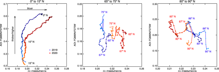
Figure 6. Color and atmospheric opacity indices for 2019 and 2020 brightness scans. Left: near the equator, there is only a slight variation in AOI, but the CI increases from 2019 to 2020 at latitudes below 10° N. Middle: near the polar storm latitudes, CI increases, and there are slight changes in the AOI, but the scale is compressed relative to that of the equator. Right: at polar latitudes, the trend is reversed and the CI decreases.
Download figure:
Standard image High-resolution imageFor temporal variation, the CI at the equator increased 9% from 2019 (blue plus symbols) to 2020 (red diamond symbols), while the AOI is unchanged (3%) to within the uncertainties. This indicates that the tropospheric clouds and haze were slightly bluer in 2020, even though all wavelengths saw a brightness increase; see Figure 2. At 65° N, the CI and AOI increased by 10% and 4%, respectively, while at 75° N, the CI increased by 7% and AOI decreased by 8%. The change in CI from 2019 to 2020 was an increase (blueshift) at 75° N and a decrease (redshift) at 80° N. The full polar region shows a redward shift of ∼7%, with 90° N showing the largest AOI increase (16%). As noted above, the FQ889N I/F is low (0.02) in the polar regions, so a large shift in AOI is still only a small change in cloud altitude or opacity.
4. Discussion
From 2019 to 2020, the equator changed more in CI than AOI, and this is also apparent in the individual filter profiles; see Figure 2. All filters from ∼400 to 760 nm show increased reflectance at the equator, while the UV and strong methane band filters sensitive to higher altitudes show little reflectance change. At the same time, both PC1 and PC2 have increased, indicating a potential change in the tropospheric and stratospheric haze optical depths (Karkoschka & Tomasko 2005; West et al. 2009). The choice of color assignment is arbitrary in the principal component analysis false-color map (Figure 4, bottom), but only the equator appears completely bright yellow: a combination of high PC1 amplitude at nonpolar latitudes (0°–60° N) indicative of thick tropospheric clouds/hazes, and high PC2 amplitude in the equatorial zone (0°–15° N) indicative of high stratospheric haze opacity. Changes from year to year are limited to within 5°–7° of the equator. Middle latitudes are dominated by PC1 (red in the false-color map and higher values in Figure 5), indicating less haze than at the equator.
Our results capture widespread changes following a major storm system in 2018, which comprised four sequential outbreaks between March and August from 67° to 74° N planetographic latitude (Sánchez-Lavega et al. 2020). The storm plumes themselves appear yellow/orange in the 2018 PC color map (Figure 4 bottom), suggesting local similarities to the equatorial aerosol structure, with high cloud opacity and high stratospheric haze opacity. But the zonal expansion of the storm activity produced global-scale changes to the aerosol structure. The latitude profile of PC1 (Figure 5) suggests a decrease of zonal cloud opacity south of the storms (∼60° to 67° N) from 2018 to 2019, with a 2020 profile of PC1 very similar to 2019. Within and north of the storm area itself (∼67° to 78° N) on the other hand, the PC1 profile suggests an increase in zonal cloud opacity from 2018 to 2019, followed by a decrease to intermediate levels by 2020. The magnitudes of the initial changes in PC1 to the south of the storm region and within/north of the storm region are approximately equal (though of opposite sign), but the relaxation back to 2018 conditions may have a longer timescale in the southern band. The combined spatial and temporal variabilities in the PC2 profile in this latitude range are smaller and more difficult to interpret, and the color changes in the overall ∼60° to 78° N region of the PC map (Figure 4, bottom) are dominated by changes in PC1 and PC3. Changes in CI for this region (Figure 6, middle) also show that the evolution of tropospheric cloud properties in the storm region continued from 2019 to 2020, after the 2018 storm eruptions themselves had ceased. From 2020 March to May, new storm outbreaks took place at ∼76° N (Sánchez-Lavega et al. 2021), and they could be responsible for the aerosol changes observed at these latitudes.
Close to the pole (≳80° N), tropospheric cloud opacity may have decreased slightly, as suggested by the 2019–2020 shift in CI (Figure 6, right). The brightness scans (Figure 2) show that most of this change is due to decreased reflectivity at blue/UV wavelengths. The false-color map shows these latitudes have a different contribution from PC2 and PC3 than other regions, with a smaller contribution from PC1 relative to the equator (Figure 5). In the PCs, the temporal change is also subtle, with a very slight decrease in PC1 from 80° to 90° N. The enhanced reflectivity maps (Figure 3, top) show that a thin blue line at 80° N (near the polar hexagon boundary) was abolished between 2019 and 2020. Both PC1 and PC2 increased during this period, with the larger change in PC2.
Changes in optical depth or color at the northern polar latitudes and the equator may not have the same causes. To determine if any of the observed changes are due to atmospheric circulation changes, we also computed zonal winds using five F631N image pairs for each year with the two images separated by a planetary rotation. All of the measurements were obtained with a cloud correlation algorithm (Hueso et al. 2009) applied over cylindrical maps of the images and using different selections of correlation parameters on different areas of the images. Obvious cloud mismatches found by the correlation algorithm were removed manually (e.g., negative winds at the equator or wind points more than 150 m s−1 different than the mean wind profile in the global analysis of winds for each year). This resulted in 7098 wind measurements in 2018, 6382 in 2019, and 5720 wind measurements in 2020, which were used to compute the meridional profile of zonal winds each year; see Figure 7.

Figure 7. Variation in Saturn's northern zonal winds and solar insolation. (A) Computed Hubble zonal wind profiles plotted over the Cassini mean profile. (B) Solar insolation pattern from 2000 to 2030 including heliocentric range and orbital inclination, but ignoring ring shadows, which have the biggest northern hemisphere effect in 2000–2006 and 2028–2030. As Saturn moves from northern winter through summer solstice in 2017, the polar insolation levels change dramatically. (C) Latitude profiles of insolation from 2006, 2018, 2019, and 2020.
Download figure:
Standard image High-resolution image
Although there are slight differences in wind jet peak magnitude from year to year, most are artifacts due to few measurable points where cloud tracers have poor contrast in many of the images, leading to large error bars. Additionally, some latitudes are prone to false detections; for example, the polar jet at 79° N, which is the location of Saturn's polar hexagon, is not well resolved and the correlation finds many measurements linked to the large-scale structure of the hexagon and not the small-scale fast-moving cloud features that define the jet. False detections are also found beyond 83degN due to the unfavorable geometry for the cloud correlation algorithm. The three wind profiles are equivalent at most latitudes within their respective error bars.
The only latitudes with significant wind velocity changes are near the equator, which is also the location showing the biggest difference from Voyager to Cassini (Sánchez-Lavega et al. 2000, 2003, 2004; Porco et al. 2005; García-Melendo et al. 2011; Sánchez-Lavega et al. 2016; Hueso et al. 2020). The Hubble-measured values were highest in 2018 and are linked to particular bright features that are easy to correlate in the images; their velocity difference is above the uncertainties. The bright features visible in 2018 are similar to the bright equatorial clouds in 2015 described by Sánchez-Lavega et al. (2016) and move at comparable speeds. At all other latitudes in the equatorial zone, weaker wind jets are also solutions within the large error bars of ∼40 m s−1. All three data sets find equatorial winds that are higher than those measured during the Cassini (2004–2009) era (García-Melendo et al. 2011). These higher winds are similar to those found in HST observations obtained in 2015, where faster motions were tied to discrete bright features that were interpreted as having deep roots one or two scale heights below the main level sampled in Cassini images (Sánchez-Lavega et al. 2016). The fastest points in our 2018–2020 data correspond to similar discrete bright features observed in 2018 (one of these can be seen in the 2018 data at 5° N latitude and 110° W longitude in Figure 3), while the 2019 and 2020 data show intermediate wind speeds not associated with particularly bright storms. This overall increase in zonal winds may be consistent with cloud contrasts in the equatorial zone lying about one scale height below the levels observed by Cassini (see Figure 8 in Sánchez-Lavega et al. 2016). Alternatively, they could be related to the 13–17 yr quasi-periodic oscillations (Fouchet et al. 2008), but further time coverage is needed to make any convincing correlation over time. While the wind field may not be directly responsible for color or opacity/altitude changes at the equator, the waves responsible for the oscillations, as well as corresponding thermal changes, may also affect the tropospheric and stratospheric aerosols.
Although the 2018 to 2020 wind changes are largest near the equator, this is likely unrelated to the seasonal solar insolation pattern from the Cassini era to the present. Cassini arrived at Saturn just past the northern winter solstice; see Figure 7(B). Although the ring shadow can strongly affect the northern midlatitude insolation when the subsolar latitude is poleward of ∼20° S, it is negligible near the summer solstice as shown in Barnet et al. (1992), Moses & Greathouse (2005), Sánchez-Lavega et al. (2020), and references therein. The Hubble observations began just after the 2017 northern summer solstice, and over the 2018 to 2020 time period, the equatorial insolation has changed little; see Figure 7(C). At this time, there appears to be no connection between insolation and equatorial cloud structure as there are only very small changes observed either by filter ratio indices or principal components.
However, sunlight at the polar regions evolves rapidly (Figure 7(C)), with a distinct change in the latitudinal insolation profile between 2019 and 2020. The abrupt polar latitude color/optical depth changes may be due to the rapidly changing sunlight levels affecting stratosphere and troposphere aerosol properties. The earliest Hubble images of Saturn in 1994 showed blue high southern latitudes, while at Cassini's 2004 arrival at Saturn, the north pole was blue in color, before gradually changing to yellow with the seasons (West et al. 2009). While only the northern latitudes are shown in this paper, the 2020 view of Saturn from Hubble included a small sliver of high southern latitudes, and they also appear blue at this time (https://hubblesite.org/contents/media/images/2020/43/4713-Image), indicating that this change is cyclical and affects both poles. Polar region dynamical changes are still possible but cannot be proven with the Hubble data at present.
5. Summary
We analyzed Hubble imaging data of Saturn from 2018 to 2020 at wavelengths from 225 to 889 nm. Using latitudinal I/F profiles at each wavelength, principal component analyses, and filter ratio indices, we have trended short-term changes in reflectance and color after the northern summer solstice. The largest apparent changes occurred at equatorial and high northern latitudes.
The equator became brighter at wavelengths from ∼400 to 760 nm, which are most sensitive to tropospheric cloud opacity. Using filter ratios, the cloud color is very slightly bluer in 2020; however, there are no changes, within the uncertainties, in cloud height or opacity. However, the principal component analysis does indicate a possible slight increase in tropospheric and stratospheric haze optical depths has occurred. As the two methods are potentially sensitive to different altitudes or particle sizes, further evolution of this region with season should reveal the cause for equatorial brightening.
At high northern latitudes, the 60°–75° N region was perturbed by storms in 2018 and 2020. These storms caused apparent cloud color changes, as well as increased stratospheric haze opacity and altered aerosol particle sizes. Further north, the polar region has progressed to redder colors, with possible changes in cloud opacity. This region should continue to evolve as solar insolation rapidly changes over time.
Zonal wind profiles were also computed, and changes were compared with solar insolation variation. The zonal winds from HST images are similar to the results from Cassini at most latitudes, despite the large difference in solar insolation. Differences in polar latitude winds are possibly artifacts from the lack of spatial resolution and polar geometry, while differences in the equatorial zone are possibly real and may merit further study in the future. When connected with Voyager-era observations, these spacecraft data sets span approximately 1.5 Saturn years, albeit with gaps in coverage. Continued Hubble observations from the OPAL program will be crucial for understanding Saturn's seasonal evolution in the post-Cassini era.
This work used data acquired from the NASA/ESA HST Space Telescope, associated with the OPAL program (PI: Simon, GO15262, GO15502, GO15929), with support provided by the Space Telescope Science Institute, which is operated by the Association of Universities for Research in Astronomy, Inc., under NASA contract NAS 5-26555. All maps are available at 10.17909/T9G593. A.S.L. and R.H. were supported by the Spanish projects PID2019109467GB-I00 (MINECO/FEDER, UE) and Grupos Gobierno Vasco IT-1366-19.