


 t 19 c 4000 Liège 1, Belgium

Abstract
We present an analysis of IRTF-TEXES spectra of Jupiter's mid-to-high latitudes in order to test the hypothesis that the CH4 homopause altitude is higher in Jupiter's auroral regions compared to elsewhere on the planet. A family of photochemical models, based on Moses & Poppe (2017), were computed with a range of CH4 homopause altitudes. Adopting each model in turn, the observed TEXES spectra of H2 S(1), CH4, and CH3 emission measured on 2019 April 16 and August 20 were inverted, the vertical temperature profile was allowed to vary, and the quality of the fit to the spectra was used to discriminate between models. At latitudes equatorward of Jupiter's main auroral ovals (>62°S, <54°N, planetocentric), the observations were adequately fit assuming a homopause altitude lower than ∼360 km (above 1 bar). At 62°N, inside the main auroral oval, we derived a CH4 homopause altitude of  km, whereas outside the main oval at the same latitude, a 1σ upper limit of 370 km was derived. Our interpretation is that a portion of energy from the magnetosphere is deposited as heat within the main oval, which drives vertical winds and/or higher rates of turbulence and transports CH4 and its photochemical by-products to higher altitudes. Inside the northern main auroral oval, a factor of ∼3 increase in CH3 abundance was also required to fit the spectra. This could be due to uncertainties in the photochemical modeling or an additional source of CH3 production in Jupiter's auroral regions.
Export citation and abstract BibTeX RIS

Original content from this work may be used under the terms of the Creative Commons Attribution 4.0 licence. Any further distribution of this work must maintain attribution to the author(s) and the title of the work, journal citation and DOI.
1. Introduction
The polar atmosphere of Jupiter is strongly influenced by the external magnetosphere and interplanetary environment. Energetic particles from the magnetosphere (and potentially the solar wind) deposit their energy in the form of particle precipitation, chemical heating, ion drag, and Joule heating (e.g., Grodent et al. 2001; Badman et al. 2015). This ultimately drives auroral emissions at X-ray, ultraviolet (e.g., Lyα), and near-infrared (H ) emissions (e.g., Gérard et al. 2014; Dunn et al. 2017; Johnson et al. 2018). A significant amount of energy is deposited as heat as deep as the 1 mbar level in the lower stratosphere (Kim et al. 1985; Kostiuk et al. 1993; Sinclair et al. 2017). The influx of energetic electrons/ions also modifies the chemistry of the atmosphere and preferentially enriches the concentrations of unsaturated and aromatic hydrocarbons, such as ethylene (C2H4), methylacetylene (C3H4), and benzene (C6H6; Sinclair et al. 2018, 2019a).
The Juno spacecraft arrived in orbit around Jupiter in 2016 July and (at the time of writing) continues to investigate the interplay between Jupiter's ultraviolet auroral emissions, the dynamics within the Jovian magnetosphere, and the influence of the external solar-wind environment (Bagenal et al. 2017). In situ measurements of the external magnetosphere are performed using the Jovian Auroral Distributions Experiment (JADE; McComas et al. 2017), Jupiter Energetic Particle Detector Instrument (JEDI; Mauk et al. 2017), Magnetometer (MAG; Connerney & Acuna 2008), and Waves (Kurth et al. 2017). Spectroscopy of the  and ultraviolet auroral emissions is performed using the Jovian Infrared Auroral Mapper (Adriani et al. 2017) and Ultraviolet Spectrometer (Gladstone et al. 2017), respectively. The ultraviolet auroral emissions are also independently studied using the Hubble Space Telescope (HST) and the Hisaki spacecraft (e.g., Tao et al. 2016; Kimura et al. 2017; Nichols et al. 2017; Grodent et al. 2018; Yao et al. 2019). Typical analyses involve inverting the spectra of the ultraviolet auroral emissions and assuming a model atmosphere of the vertical hydrocarbon distributions to derive characteristic energies of the precipitating electrons driving the emissions. These derived energy fluxes are then compared with the in situ measurements by Juno-JADE/JEDI. The comparison reveals whether the downward or upward electron fluxes are sufficient in magnitude to drive the observed auroral emissions and infer the presence of acceleration regions in the magnetosphere between the planet and the spacecraft. One source of uncertainty in the inversion of the ultraviolet spectra is the vertical distributions of the hydrocarbons and how high in altitude they can be transported, specifically the altitude of the CH4 homopause (e.g., Gérard et al. 2014; Yao et al. 2019). The homopause marks the altitude where eddy and molecular diffusion rates become equal.
The altitude of the CH4 homopause is not uniquely constrained near Jupiter's poles; however, several studies of the auroral emissions have inferred that it is at a higher altitude in Jupiter's auroral regions compared to elsewhere on the planet. For example, Parkinson et al. (2006) analyzed Cassini Ultraviolet Imaging Spectrometer (UVIS; Esposito et al. 2004) observations of Jupiter's helium airglow emission and derived eddy diffusion coefficients up to an order of magnitude higher than those derived at equatorial latitudes. Using HST Space Telescope Imaging Spectrograph measurements, Gustin et al. (2016) demonstrated that ultraviolet emissions from the Io footprint exhibited signatures of hydrocarbon absorption, which would require an upward shift of the hydrocarbon homopause of at least 100 km. A recent study by Clark et al. (2018) compared observations measured by Juno-JEDI and characteristic electron fluxes inverted from Hisaki Extreme Ultraviolet Spectroscope for Exospheric Dynamics (Yoshioka et al. 2013) ultraviolet observations of Jupiter's aurora. They found that the agreement between the electron energy distributions inverted from the ultraviolet observations and those measured by JEDI was optimized when a model atmosphere was assumed that allowed CH4 and other hydrocarbons to be transported to higher altitudes.
In contrast, Kim et al. (2017) analyzed 3 and 8 μm (∼3030 and ∼1250 cm−1) CH4 emissions and derived a vertical profile of CH4 that was similar to the profile derived at equatorial regions (Kim et al. 2014) and relatively depleted of CH4 at higher altitudes. In addition, in a steady state, the altitude of the CH4 homopause would be expected to be lower in Jupiter's auroral regions. While the rate of eddy diffusion is dependent on vertical and horizontal temperature gradients, the molecular diffusion exhibits a 0.765 power-law dependence on temperature. In Jupiter's auroral regions, the transition from the near-isothermal mesosphere to the strong temperature increase associated with the thermosphere occurs at lower altitudes/higher pressures (e.g., Bougher et al. 2005; Sinclair et al. 2018). Thus, the molecular diffusion coefficient would be expected to increase sharply at the base of the thermosphere and thereby meet the eddy diffusion coefficient at a higher pressure/lower altitude and decrease the altitude of the CH4 homopause. However, the atmosphere in Jupiter's auroral regions is likely far from a steady state and far different compared to lower-latitude regions due to the highly variable influence of the magnetosphere and interplanetary environment. It is possible that regular injections of energy from the magnetosphere ultimately result in CH4 and other hydrocarbons being lofted to higher altitudes (Grodent et al. 2001). In Sinclair et al. (2019b), a brightening of Jupiter's southern auroral 7.80 μm (∼1280 cm−1) CH4 emission was observed during a solar-wind compression. One suggested explanation was that the solar-wind compression perturbed the magnetosphere such that energy was deposited into the neutral atmosphere and produced vertical winds that transported CH4 to higher and warmer altitudes, thereby enhancing its emission. If such a process occurred regularly, this could give the impression that the CH4 homopause is higher in altitude, though advection, not diffusion, is the mechanism responsible.
In this study, we test the hypothesis that the CH4 homopause is at a higher altitude in Jupiter's auroral regions. The addition of a filter to the Texas Echelon Cross Echelle Spectrograph (TEXES; Lacy et al. 2002) instrument on NASA's Infrared Telescope Facility (IRTF) has improved the sensitivity at ∼16 μm (∼606 cm−1) and allowed the emission of CH3, the methyl radical, to be measured. The CH3 is produced predominantly from ultraviolet photolysis of CH4, and, as demonstrated in this paper, its vertical profile/concentration is sensitive to the location of the CH4 homopause. By performing an analysis of CH4 and CH3 emission spectra measured by TEXES, we can provide constraints on the location of the CH4 homopause and its variation as a function of latitude, longitude, and particularly contrasts inside and outside Jupiter's main auroral ovals.
2. Observations
The IRTF-TEXES high-resolution (65,000 < R < 85,000) spectra were measured on 2019 April 16 and August 20 UTC. As detailed in previous work (e.g., Fletcher et al. 2016; Sinclair et al. 2018), the slit of the instrument is stepped across Jupiter's mid-to-high northern latitudes (poleward of 45°N) in steps of 0 7 (for Nyquist sampling) in order to map the emission in a given spectral setting over all visible longitudes. This procedure is repeated for several discrete spectral settings before duplicating the measurements for mid-to-high southern latitudes. This is repeated over the course of a night, while Jupiter is below an airmass of 2, in order to use Jupiter's rotation (with a period of 9 hr 50 minutes) to build up longitudinal coverage.
These observations were performed as part of a longer-term program to measure the spectral emission features of the H2 S(1) quadrupole, C2H2, C2H4, C2H6, and CH4 and their variability at Jupiter's high latitudes. In this paper, we focus only on the spectra measured in settings centered at 587, 606, and 1248 cm−1, which target H2 S(1), CH3, and CH4 emission, respectively. Spectra of other emission features and/or measured on different dates will be presented in a future publication. Tables A1 and A2 further detail the observations analyzed in this study.
For each observation, the wavelength-dependent noise was calculated by finding the standard deviation of all sky pixels more than 2'' away from the planet. This calculation of noise captures instrument sensitivity and variations in sensitivity during/between nights due to changing observation conditions and assigns higher noise values to spectral regions of lower telluric transmission, which are weighted less in all subsequent analyses.
In previous analyses of TEXES high-resolution spectra (e.g., Sinclair et al. 2018), a scale factor of 1.3 was applied to all 587 cm−1 spectra in order to optimize the simultaneous fit of the observed H2 S(1) quadrupole and CH4 emission with the same temperature profile. This was attributed to errors in the calibration of the spectra and/or beam dilution due to diffraction near the limb of the planet. In this study, we found that a scale factor of 1.3 was also needed to simultaneously fit the H2 S(1) quadrupole and CH4 emission observed on both 2019 April 16 and August 20. Spectra measured in the 606 cm−1 setting were scaled by factors ranging from 1.0 to 2.0 in increments of 0.05, and the simultaneous fit of the continua in the 587 and 606 cm−1 settings was tested at a range of latitudes. We found that a scale factor of 1.4 was needed to best fit the continua in the 587 and 606 cm−1 settings simultaneously. The results presented in the main body of this paper are derived from spectra, where the 587 and 606 cm−1 settings were scaled by factors of 1.3 and 1.4, respectively.
All target spectra higher than 80° in emission angle were omitted in order to avoid locations where diffraction was mixing dark space and emission from the planet. In order to improve the effective signal-to-noise ratio (S/N), individual spectra were coadded in several ways, as detailed below. The effective noise spectra on the coadds were calculated by adding the noise on individual spectra in quadrature.
Nonauroral longitudinal mean. In a given spectral setting, individual spectra were sorted into 4° wide (planetocentric) latitude bins Nyquist sampled by 2°. Spectra were coadded while omitting spectra measured at longitudes from 140°W to 240°W (system III) in the north and 330°W to 90°W in the south, which conservatively removes spectra measured close to/inside each auroral region (Bonfond et al. 2017). All latitudes and longitudes quoted hereafter are planetocentric and system III, respectively. For simplicity, we will describe these spectra as the "nonauroral longitudinal mean," though we caution the reader that these do not represent a true mean of all longitudes or a zonal mean. Analysis of these observations allows meridional variations of the CH4 homopause altitude to be determined but excluding longitudes directly affected by auroral processes.
Auroral mean. For latitudes poleward of 56°N, individual spectra were sorted into 4° wide (planetocentric) latitude bins Nyquist sampled by 2°, as above. In each latitude bin, spectra measured at longitudes inside the northern main auroral oval (Bonfond et al. 2017) were coadded into a single spectrum representing a mean of the auroral region in that latitude circle. We did not compute a similar mean spectrum for the south, as our observations did not sufficiently sample the longitudes inside the southern auroral oval.
Latitude–longitude binning. Individual spectra were coadded into 4° wide latitude bins Nyquist sampled by 2° and 20° longitude bins Nyquist sampled by 10°. These spectra allow both meridional and zonal variations in emission to be assessed, though at a lower sensitivity than the nonauroral longitudinal- and auroral-mean spectra. Figure 1 shows the distribution of CH3 and CH4 emission as a function of latitude and longitude for both 2019 April 16 and August 20 measurements.
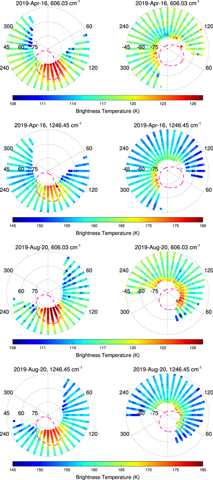
Figure 1. Polar projections of CH3 emission at 607.03 cm−1 and CH4 emission at 1246.45 cm−1 measured by TEXES on 2019 April 16 (top two rows) and 2019 August 20 (bottom two rows). The pink dashed lines mark the statistical-mean position of the ultraviolet ovals (Bonfond et al. 2017).
Download figure:
Standard image High-resolution image3. Radiative Transfer Model
3.1. Atmospheric Model
The vertical profiles of H2, He, NH3, and PH3 were adopted from Sinclair et al. (2018). The vertical profiles of temperature, CH4, CH3, C2H2, C2H4, and C2H6, were nominally adopted from a photochemical model presented in Moses & Poppe (2017). This model was nominally calculated at a latitude of 30°. The vertical profiles of CH4 and its by-products are expected to vary with latitude due to variations in the solar illumination angle and the longer path length through the atmosphere. However, such variations resulted in differences of the CH4 and CH3 abundances by a factor of 2 or less, which is within the uncertainty introduced into the model by the CH3 chemical kinetics (e.g., Dobrijevic et al. 2003, 2010). Thus, we continue to adopt the model results at 30°N for the work in this paper; we note this approximation for the reader. Eight alternative photochemical models were computed by increasing the gradient of the eddy diffusion coefficient profile at pressures lower than 10 μbars (or approximately 260 km above the 1 bar level), as shown in Figure 2. This serves to increase the altitude of the CH4 homopause, where the molecular and eddy diffusion coefficients match, and transports CH4 (and thus its photochemical by-products, including CH3) to higher altitudes/lower pressures. For the two models with the highest vertical gradient in eddy diffusion, the coefficient was truncated to 1010 cm2 s−1 so that the resulting vertical profiles of CH4 and CH3 were spaced similarly to the previous seven models. The resulting vertical profiles of CH4 and CH3 are also shown in Figure 2. For simplicity, we will label these models by number, with "model 1" being the lowest-altitude homopause model (and identical to the model presented in Moses & Poppe 2017) and "model 9" being the highest-altitude homopause model. Table 1 details the locations of the homopause for each model in altitude and pressure units and the eddy diffusion coefficient at the homopause. Although models 8 and 9 have identical homopause altitudes, their eddy diffusion profiles and thus vertical profiles of CH4 and CH3 differ greatly at altitudes below the homopause, as demonstrated in Figure 2. This is a further reason why we chose to label the models by number and not by homopause altitude.
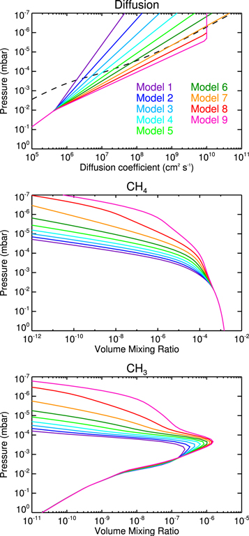
Figure 2. The top panel shows the vertical profiles of eddy diffusion (colored lines) associated with models 1–9 and the molecular diffusion profile (black dashed line) for comparison. The resulting vertical profiles of CH4 and CH3 are shown in the middle and bottom panels. Model 1 (purple) is the same model presented in Moses & Poppe (2017). The color scheme in this figure is adopted throughout the paper.
Download figure:
Standard image High-resolution imageTable 1. The Pressure Levels (in nbar) and the Eddy Diffusion Coefficient at the Homopause (KH) for the Models Tested in This Work (Figure 2)
| Model Number | Location of Homopause | KH | |
|---|---|---|---|
| Pressure (nbar) | Altitude (km) | (106 cm2 s−1) | |
| Model 1 | 294.6 | 332.1 | 1.72 |
| Model 2 | 220.0 | 342.6 | 3.06 |
| Model 3 | 165.3 | 354.1 | 5.36 |
| Model 4 | 122.8 | 367.5 | 9.23 |
| Model 5 | 67.0 | 401.1 | 26.16 |
| Model 6 | 36.0 | 441.8 | 68.94 |
| Model 7 | 7.3 | 579.9 | 566.15 |
| Model 8 | 0.5 | 623.3 | 9780.75 |
| Model 9 | 0.5 | 592.3 | 9780.75 |
Note. As an example, altitudes above the 1 bar level are quoted and were calculated from the pressure–temperature profiles retrieved from a mean of all spectra recorded between 48°N and 52°N. For a given model, homopause altitudes will vary with location depending on the retrieved vertical temperature profile and the local gravity field. Derived altitudes at specific locations are quoted throughout the text.
Download table as: ASCIITypeset image
3.2. Spectroscopic Line Data and Forward Model
The sources of spectroscopic line data for the H2 S(1) quadrupole line feature, NH3, PH3, CH4, CH3D, 13CH4, C2H2, C2H4, and C2H6, were adopted from Fletcher et al. (2018). The spectroscopic line data for CH3 was adopted from Bezard et al. (1998) and Bézard et al. (1999) but with updates to the line intensities based on Stancu et al. (2005). The CH3 vibrational partition function was calculated assuming the following modes and degeneracies: ν1 = 3004 cm−1 (g = 1), ν2 = 606 cm−1 (g = 1), ν3 = 3161 cm−1 (g = 2), and ν4 = 1396 cm−1 (g = 2).
Forward modeling and retrievals were performed using the NEMESIS radiative transfer code (Irwin et al. 2008). NEMESIS can perform forward modeling using both the line-by-line and correlated-k methods; the latter was chosen for higher computational efficiency. The k-distributions were computed for the aforementioned species from 585 to 589, 605 to 609, and 1244 to 1252 cm−1. Due to the different slit widths adopted in these settings, a 6 km s−1 sinc-squared convolution was adopted in the calculations from 585 to 589 and 605 to 609 cm−1, and a 4 km s−1 sinc-squared convolution was adopted for 1244–1252 cm−1.
3.3. Vertical Sensitivity
Synthetic spectra were computed for all nine atmospheric models (Figure 2) from 585 to 589, 605 to 609, and 1244 to 1252 cm−1 at an emission angle of 70°. Figure 3 shows the latter two ranges and demonstrates the variation of the CH3 and CH4 emission due to changes in their vertical profiles. The vertical functional derivatives with respect to temperature were calculated to determine the vertical sensitivity of the H2 S(1) quadrupole and CH3 and CH4 emission, respectively. The results are shown in Figure 4.
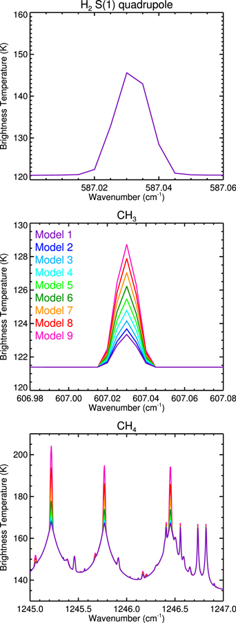
Figure 3. Synthetic spectra of H2 S(1) quadrupole (top), CH3 (middle), and CH4 (bottom) emission using the vertical profiles of each species from models 1–9 (see Figure 2). The color legend is shown in the middle panel and is identical to that shown in Figure 2. The H2 S(1) emission spectra do not differ between each model.
Download figure:
Standard image High-resolution image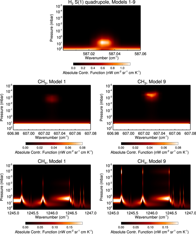
Figure 4. Vertical functional derivatives with respect to temperature for H2 S(1) emission (top panel), CH3 emission (second row), and CH4 emission (third row), which describe the relative contribution of each atmospheric level to the total observed radiance at the top of the atmosphere. Only a subset of the spectral range of CH4 emission used in this study is shown for clarity. The vertical sensitivity of H2 S(1) emission is identical for models 1–9. For CH3 and CH4 emission, results assuming models 1 and 9 (see Figure 2) are shown on the left and right, respectively. Varying the altitude of the CH4 homopause shifts the altitude of peak sensitivity in CH3 and CH4 emission in the upper stratosphere (at pressures lower than 200 μbars).
Download figure:
Standard image High-resolution imageThe H2 S(1) quadrupole emission sounds the atmosphere from approximately 50 to 1 mbar, with the continuum outside the line sounding the troposphere at 100–300 mbars (also shown previously in Fletcher et al. 2016 and Sinclair et al. 2018). The vertical sensitivity of the H2 S(1) emission does not change with respect to the CH4 homopause altitude assumed. The wings of the strong CH4 emission lines (e.g., 1245.0–1245.25 cm−1) and weaker CH4 lines (e.g., 1246.7 cm−1) sound the lower stratosphere of Jupiter from approximately 30 to 0.03 mbar. There is a negligible change in the contribution of the atmosphere at pressures higher than 200 μbars as a function of the CH4 homopause altitude.
The vertical sensitivity of the emission lines of CH3 and the cores of the strong CH4 lines exhibit a variation in altitude depending on the CH4 homopause altitude assumed. For model 1 (Moses & Poppe 2017), CH3 emission peaks in sensitivity at approximately 1.6 μbars, whereas the cores of the strong CH4 lines peak in sensitivity at approximately 9 μbars. For model 9, CH3 emission peaks in sensitivity at 0.4 μbar, and the cores of the strong CH4 lines peak in sensitivity at approximately 0.2 μbar. For a given atmospheric model, the vertical sensitivities of the CH3 and CH4 emission do overlap, but the altitudes of peak sensitivity are generally offset. This is particularly true for atmospheric models assuming a lower-altitude CH4 homopause. We explore the uncertainty this introduces into the analysis by inverting the synthetic observations in Section 4.2.
We note that a proportion of the CH4 emission and all of the CH3 emission is formed at pressure levels/altitudes where the assumption of local thermodynamic equilibrium (LTE) may no longer be valid. Due to the paucity of intermolecular collisions at lower pressures, the translational, rotational, and vibrational populations of molecules can no longer remain in equilibrium; thus, the population levels can no longer be described by the Boltzmann equation, and the source function deviates from a blackbody. However, our radiative transfer code assumes LTE. We will further discuss the potential consequences of this assumption for our results in Section 5.
4. Analysis and Results
4.1. Retrieval Approach
The magnitude of the emission features of CH3 and CH4 is dependent on the vertical profiles of temperature and their abundances. Generally, the retrieval fitting of hydrocarbon emission features, such as C2H2, C2H4, etc., is performed by retrieving the temperature profile from CH4 emission and then varying the vertical profile of the emitting hydrocarbon species (e.g., Nixon et al. 2007, 2010; Fletcher et al. 2016; Sinclair et al. 2017, 2019a). However, preliminary retrievals using this method required significant order-of-magnitude enhancements of CH3 with respect to model 1 (Moses & Poppe 2017) in order to fit its emission feature, especially in Jupiter's auroral regions. Given the close coupling of CH4 and CH3 through ultraviolet photolysis of the former, the fact that CH3 was strongly enriched would then imply that the assumed vertical profile of CH4 was incorrect. This would then imply that the vertical temperature profile, which is retrieved from the CH4 emission, is incorrect. Thus, fitting the emission features of CH3 and CH4 using this method would result in a degenerate set of solutions that were not physical.
In this paper, we instead adopted a more cautious retrieval approach. Nominally, the vertical profiles of CH3 and CH4 were adopted from models 1–9 in turn and held constant. Thus, the assumed vertical profiles of CH3 and CH4 are photochemically self-consistent. The emission features of the H2 S(1) quadrupole, CH3, and CH4 were modeled simultaneously, and only the vertical temperature profile was allowed to vary. The goal was to fit all three emission features with a physically sensible temperature profile and determine the model atmosphere that provided the optimum correspondence between the observed and modeled spectra. Using the retrieved temperature profile derived from each model and the gravity at the latitude of the observation and assuming hydrostatic equilibrium, the pressure–altitude grid was calculated. For each retrieval, the CH4 homopause altitudes associated with each model were recalculated by interpolation of the homopause pressure levels (Table 1) onto the pressure–altitude grid derived from the retrieval. The model that minimized the χ2 fit to the CH3 and CH4 emission was determined, and the corresponding CH4 homopause altitude was assumed as the result. The 1σ confidence levels on the CH4 homopause altitude were derived by finding the homopause altitudes corresponding to the (absolute) χ2 + 1 level (Press et al. 1992). For a small subset of observations, where this approach could not adequately fit the core of the CH3 emission within the 1σ noise level, we also allowed the vertical profile of CH3 to vary (Section 4.6).
4.2. Testing of Synthetic Spectra
In Section 3.3, we demonstrated that the peak sensitivity of CH3 and CH4 emission can be offset in altitude. In order to highlight the uncertainty this introduces into our analysis, we performed a retrieval analysis of synthetic spectra, where spectra are computed from a model atmosphere, noise is added to simulate an observation, and then the observations are inverted to determine whether the correct result can be retrieved.
The 1σ noise on the coadded spectra at 68°N, 180°W (near the center of the northern main oval) measured on 2019 August 20 was adopted as the effective noise spectrum. Random noise of this magnitude was then computed and added to the synthetic spectra computed for models 1–9 (the noiseless spectra are shown in Figure 3). The simulated noisy spectra of model 1 from 587.00 to 587.06, 606.95 to 607.10, 1245.19 to 1245.24, 1245.60 to 1245.80, 1246.30 to 1246.75, 1247.50 to 1247.73, 1248.20 to 1248.50, 1249.40 to 1249.68, and 1249.90 to 1250.05 cm−1 were initially adopted as the observation. These wavenumber ranges were chosen to capture H2 S(1) quadrupole, CH3, and CH4 emission and for consistency with the specific wavenumber ranges chosen in the analysis of real observations measured on 2019 August 20 (Section 4). As detailed in Section 4.1, the vertical profiles of CH3 and CH4 were fixed to those of models 1–9 in turn, and the vertical temperature profile was retrieved by simultaneously fitting the H2 S(1) quadrupole, CH3, and CH4 emission features. The retrievals were performed three times starting from different initial guesses or a priori temperature profiles: (1) the temperature profile used in computing the synthetic spectra, and thus the correct profile; (2) the correct temperature profile with an offset of −15 K at all altitudes; and (3) the correct temperature profile with an offset of +15 K at all altitudes. These procedures were then repeated for the simulated noisy spectra computed from models 2–9 in turn.
The quality of the fit of the modeled spectra to the simulated observations was quantified by calculating the reduced χ2 statistic (Equation (1)), where Oi, Mi, and σi are the observed radiance, modeled radiance, and noise at wavenumber i, respectively, and N is the number of independent spectral points:

To determine the quality of the fit to the CH3 emission, χ2/N was calculated from 607.0 to 607.05 cm−1 and for all sampled CH4 emission between 1245.19 and 1250.05 cm−1. A combined measure of the fit to both the CH3 and CH4 was also calculated over both wavenumber ranges. We also calculate the absolute χ2 statistic (as in Equation (1) but omitting the factor of 1/N) to quantify whether a given model significantly improved the quality of the fit over another model and to derive confidence levels. Deviations from the minimum (best-fitting) absolute χ2 of 1, 4, and 9 mark the location of the 1σ, 2σ, and 3σ confidence levels (Press et al. 1992). Confidence levels are converted into homopause altitude units by linear interpolation of the altitudes shown in Table 1 calculated at the appropriate latitude.
Figure 5 shows the reduced χ2/N fits to the CH3 and CH4 emission for every combination of simulated observation, model atmosphere, and a priori temperature profile. In general, when the temperature retrieval is performed using the correct temperature profile a priori, and the correct model vertical profiles of CH3 and CH4 are adopted, the fit to the CH3 and CH4 emission is optimized for the majority of simulated observations and model atmospheres tested. There are some exceptions. For example, for the observation simulated from model 9 (the highest-altitude CH4 homopause model), adopting the vertical profiles of CH3 and CH4 from model 5 yields the best fit (χ2/N = 0.537) compared to the correct model atmosphere (χ2/N = 0.581). This is true even when performing the retrieval from the correct temperature profile a priori. This is an artifact that arises from the double-peaked nature of the CH4 contribution function and the offset in peak sensitivity of the CH3 and CH4 emission for a given atmospheric model (Figure 4). However, for the observation simulated using model 9, adopting the vertical profiles of CH3 and CH4 from model 5 yields a χ2/N = 1.729 to the CH4 emission, whereas adopting the correct model (model 9) yields a value of 0.736. Thus, equally weighting the quality of the fit to both the CH3 and CH4 emission allows such examples of false χ2 minima to be rejected. This is also demonstrated in the third column of Figure 5.
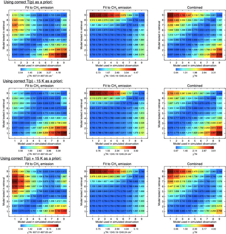
Figure 5. Retrievals of simulated observations. Each panel shows two-dimensional grids of reduced χ2 fits to the CH3 (left column) and CH4 (middle) emission and the combined fit to the CH3 and CH4 emission (right), with the x-axes representing the model atmosphere simulated and the y-axes representing the model atmosphere tested in the retrieval of the temperature profile. The top row shows the results when the correct temperature profile is adopted as the a priori, and the second and third rows, respectively, show results when an a priori temperature profile, which is offset at all altitudes from the correct profile by 15 or −15 K, is adopted.
Download figure:
Standard image High-resolution imageWhen starting the retrieval from an a priori offset from the correct temperature profile, the reduced χ2 fit to the observations does not reach a minimum value using the correct atmospheric model. In performing the temperature retrievals using an a priori that is cooler than the correct profile, the reduced χ2/N will tend to minimize using an atmospheric model with a higher homopause altitude than the correct model. The converse is true when starting from an a priori profile that is warmer than the correct profile. However, the difference in χ2 between the best-fitting model and the correct model is generally negligible. For example, for the observation simulated from model 5, in performing the temperature retrieval using an a priori that is cooler than the correct profile, the minimum χ2/N = 0.686 (best fit) is achieved using model 6, while using model 5 (the correct model) yields χ2/N = 0.704. In absolute χ2, the minimum χ2 = 10.976 is achieved using model 6, and the location of  + 1 in parameter space marks the location of the 1σ confidence level (Press et al. 1992). Thus, both model 5 (the correct model) and model 6 yield fits to the simulated observation of similar quality.
Thus, the offset in pressure/altitude of the peak sensitivities in the CH3 and CH4 emissions does introduce uncertainty into the analysis performed in this work. However, this uncertainty can be highlighted and quantified by (1) performing the retrievals from different a priori profiles and (2) quantifying the variation in absolute χ2 as a function of model to capture all models that fit the observations within the 1σ confidence level. Nevertheless, this analysis of simulated observations demonstrates that testing the quality of the fit to the CH3 and CH4 emission as a function of the atmospheric model assumed does indeed allow relative variations in the homopause altitude to be correctly determined. It should also be noted that the observations simulated in this section represent a worst-case scenario in sensitivity. The spectra were forward-modeled assuming a temperature profile representative of Jupiter's equatorial regions, which is missing the stratospheric heating present in Jupiter's auroral regions (Kim et al. 1985; Sinclair et al. 2017, 2018). In reality, the thermal emission of CH3 and CH4 at higher latitudes would be enhanced due to the warmer line-forming region. In addition, the noise added to simulate the observations captures the effective noise on a spectrum over 20° in longitude and 4° in latitude. For nonauroral longitudinal- and auroral-mean spectra (see Section 2), a greater number of spectra are averaged together; thus, the sensitivity would be significantly higher than the level tested in this section.
4.3. Meridional Variations Outside the Auroral Region
The retrieval approach described in Section 4.1 was performed for all nonauroral longitudinal-mean spectra measured on 2019 April 16 and August 20. As in Section 4.2, the χ2 statistics (Equation (1)) were calculated from 607.0 to 607.05 and 1245.19 to 1250.05 cm−1 to quantify the goodness of fit to the CH3 and CH4 emission, respectively. Figure 6 shows the retrieved temperature results from the August 20 measurements and the goodness of fit to the CH3 and CH4 emission for all nine models. The results for 2019 April 16 are very similar to those of August 20 and are shown in Figure B1 in Appendix B.
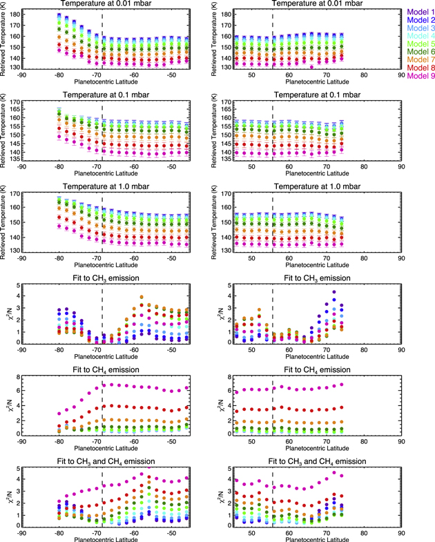
Figure 6. Nonauroral longitudinal-mean retrievals of temperature from TEXES measurements on 2019 August 20 as a function of latitude in the south (left column) and north (right column). The results are colored according to the model profiles of CH3 and CH4 adopted as shown in the legend (and identical to the color scheme shown in Figure 2). Temperatures at 0.01, 0.1, and 1.0 mbar are shown in the first, second, and third rows, respectively. The fourth, fifth, and sixth rows show the reduced χ2 fit to the CH3 emission feature from 607.01 to 607.05 cm−1, all sampled CH4 emission from 1245.19 to 1250.05 cm−1, and the combined fit to the CH3 and CH4 emission, respectively. In all panels, the vertical dashed lines mark the lowest-latitude extent of the main ultraviolet auroral ovals (Bonfond et al. 2017).
Download figure:
Standard image High-resolution imageFor results from a single model, temperatures are relatively constant as a function of latitude in the northern hemisphere. In the southern hemisphere, temperatures are also constant with latitude until approximately 64°S and then exhibit an increase toward higher latitudes, in particular at lower pressures. Taking into account the diffraction of the observations and the 4° wide latitude binning of the spectra, the location of this heating is well correlated with the latitudinal extent of the southern auroral oval. Even though these observations do not directly sample the longitudes inside the southern auroral oval, auroral-related heating is obviously advected horizontally to other longitudes.
Since the vertical temperature profile is predominantly derived from the CH4 emission, assuming different vertical profiles of CH4 yields a range of retrieved temperatures, with lower temperatures retrieved using a model with a higher-altitude CH4 homopause and higher temperatures retrieved using a lower-altitude CH4 homopause. The differences in the retrieved temperatures are largest at the lowest pressures, where the CH4 abundance differs most between models. The choice of model still affects retrieved temperatures at 1 mbar due to the double-peaked nature of the contribution function of CH4 emission (Figure 4). For example, at 50°N, at 0.01 mbar, a temperature of 158.9 ± 1.6 K is retrieved using model 1 (Moses & Poppe 2017), while a temperature of 134.7 ± 2.2 K is retrieved using model 9. In contrast, at 1.0 mbar, a temperature of 154.7 ± 1.4 K is retrieved using model 1, while a temperature of 136.6 ± 1.8 K is retrieved using model 9.
At latitudes equatorward of 62°S and 54°N, model 1 (the lowest-altitude CH4 homopause model; Moses & Poppe 2017) yields the best fit to both the CH3 and CH4 emission. This is exemplified for 50°N in Figure 7, which compares the observed and modeled spectra using model 1 (the best-fitting model) and the corresponding retrieved temperature profile. The results for models 5 and 9 and the corresponding temperature retrievals, which reveal relatively poorer fits, are also shown for comparison. Figure 8 shows the variations in absolute χ2 for 50°N and 60°S as a function of the model tested and also demonstrates that model 1 is the best-fitting model at both locations. Adopting the pressure–altitude grid derived from each retrieval (calculated from hydrostatic equilibrium, the retrieved vertical temperature profile, and the local gravity field), model 1 corresponds to CH4 homopause altitudes (above the 1 bar level) of 332 and 323 km at 50°N and 60°S, respectively. Since model 1 is also the lowest-altitude CH4 homopause model tested in this study, we cannot determine a lower confidence level on the homopause altitude that best fits the observations. However, by linear interpolation of the homopause altitudes derived from each model, we derive an upper 1σ confidence level of 357 and 341 km (above 1 bar) for the CH4 homopause altitude at 50°N and 60°S, respectively.
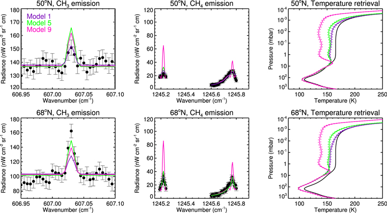
Figure 7. Comparisons of observed and modeled spectra at the corresponding retrievals of temperature for nonauroral longitudinal-mean observations at 50°N (top row) and 68°N (bottom row). The a priori temperature profile is shown in black in both rows. As shown in Figure 6, adopting the vertical profiles of CH3 and CH4 from model 1 yields the best fit to the observed spectra at 50°N ,whereas model 5 yields the best fit to the spectra at 68°N. Poorer-fitting models are also shown for comparison.
Download figure:
Standard image High-resolution image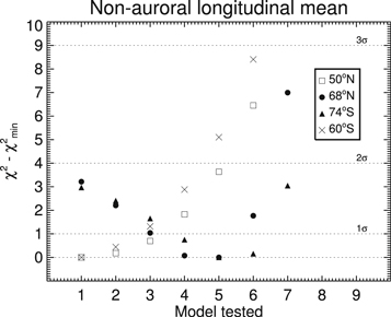
Figure 8. Absolute χ2 values of both the CH3 and CH4 emission, with respect to the minimum χ2, as a function of atmospheric model tested for nonauroral longitudinal-mean observations on 2019 August 20 at 50°N (open squares), 68°N (filled circles), 60°S (crosses), and 74°S (triangles). Horizontal dashed lines mark the 1σ, 2σ, and 3σ confidence levels. Only the zero to 3σ range is shown; missing results are outside this range.
Download figure:
Standard image High-resolution imageAt higher latitudes, the fit to the observations using lower-altitude homopause models deteriorates, particularly for the CH3 emission. This transition occurs at approximately 64°S and 54°N. Taking into account blurring of the observations due to diffraction and the 4° wide latitudinal binning of the coadded spectra, the locations of these transitions in each hemisphere are well correlated with the latitudinal extent of the northern and southern auroral regions poleward of 55°N and 69°S, respectively (Bonfond et al. 2017). Even though the spectra in this section do not sample the longitudes inside the main auroral ovals, horizontal advection and diffusion allows processes related to the aurora to affect a large range of longitudes in a given latitude band.
At both 74°S and 68°N, the vertical profiles of CH3 and CH4 of model 5 optimize the fit to the observations, especially the CH3 emission. This is also exemplified in Figure 7 for 68°N, which compares the observed spectra and the modeled spectra using model 5 (the best-fitting model) and the corresponding retrieved temperature profile. The results for poorer-fitting models 1 (the best-fitting model at lower latitudes) and 9, and the corresponding temperature retrievals, are also shown for comparison. Figure 8 also shows the variations in absolute χ2 for 68°N and 74°S as a function of the model tested. In both locations, models 4–6 produce comparable fits to the observations, but models 1–3 and 7–9 lie outside the 1σ confidence level. Adopting the pressure–altitude grid derived from each retrieval, we derive homopause altitudes of  km at 68°N and
  km at 74°S.
4.4. Longitudinal Variations at High Northern Latitudes
In the previous section, we demonstrated that a higher-altitude CH4 homopause is required to fit longitudinal-mean observations at latitudes poleward of 64°S and 54°N but excluding the longitudes inside the auroral ovals. In this section, we seek to determine whether longitudinal variations in CH4 homopause altitude exist in a given latitude circle poleward of 54°N. In Section 4.4.1, we compare the results derived from nonauroral longitudinal- and auroral-mean spectra (see Section 2) to determine whether there is a contrast in the CH4 homopause altitude inside and outside the auroral region in a given latitude band. In Section 4.4.2, we search for spatial variations in CH4 homopause altitude inside the northern auroral oval. We do not attempt a similar analysis for the south, since our observations did not sufficiently sample the southern auroral oval.
4.4.1. Contrasts Inside/Outside the Northern Auroral Oval
The retrieval approach described in Section 4.1 was performed for all auroral-mean observations (see Section 2). Figure 9 shows retrieved temperatures from the August 20 measurements and the goodness of fit to the CH3 and CH4 emission for all nine atmospheric models.
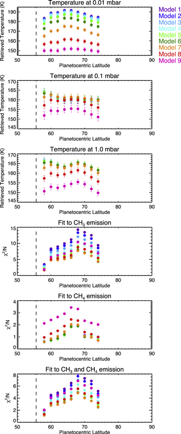
Figure 9. Auroral-mean retrievals of temperature from TEXES measurements on 2019 August 20. The results are colored according to the model profiles of CH3 and CH4 adopted as shown in the legend (and identical to the color scheme shown in Figure 2). Temperatures at 0.01, 0.1, and 1.0 mbar are shown in the first, second, and third rows, respectively. The fourth, fifth, and sixth rows show the reduced χ2 fit to the CH3 emission feature from 607.01 to 607.05 cm−1, all sampled CH4 emission from 1245.19 to 1250.05 cm−1, and the combined fit to the CH3 and CH4 emission, respectively. The vertical dashed lines mark the lowest-latitude extent of the main ultraviolet auroral ovals.
Download figure:
Standard image High-resolution imageAs for nonauroral longitudinal-mean observations (Section 4.3), the choice of atmospheric model changes the absolute temperature retrieved, particularly at higher altitudes/lower pressures. At all latitudes inside the main oval, models 6 or 7 provide the best fit to the observed CH3 and CH4 emission. However, with the exception of the observations at 58°N, we could not obtain adequate fits to the CH3 emission feature at 607.03 cm−1 by varying only the vertical temperature profile. This is resolved in Section 4.6, when we allow the vertical profiles of both temperature and CH3 to vary.
Figure 10 shows variations in absolute χ2 with respect to the minimum χ2 at 62°N, 66°N, and 70°N for longitudes outside and inside the auroral region. At 62°N, sampling longitudes outside the auroral region, model 2 optimizes the fit to the observations, while models 1, 3, and 4 also provide adequate fits. Adopting the pressure–altitude grid derived for each retrieval and by interpolation of the homopause pressure levels for each model (Table 1), we derive a CH4 homopause altitude of 331 km above the 1 bar level with an altitude of 370 km marking the upper 1σ confidence level. We could not calculate a lower 1σ confidence level from the models tested at this location. At 62°N, using a mean of all observations sampled inside the northern auroral oval, model 6 provides the best fit to the observations. From the pressure–altitude grid derived from each retrieval, we derive a homopause altitude of  km above the 1 bar level. Thus, at 62°N, we can conclude that the CH4 homopause altitude inside the auroral oval is 130 ± 55 km higher compared to longitudes outside the main oval.
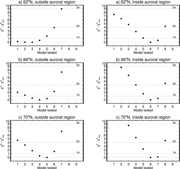
Figure 10. Absolute χ2 values of both the CH3 and CH4 emission, with respect to the minimum χ2, as a function of atmospheric model tested for nonauroral longitudinal-mean (left column) observations on 2019 August 20 at 62°N (first row), 66°S (second row), and 70°N (third row) and auroral-mean observations (right column) at the same latitudes. Horizontal dashed lines mark the 1σ, 2σ, and 3σ confidence levels. Only the zero to 3σ range is shown; missing results are outside this range.
Download figure:
Standard image High-resolution imageAt higher latitudes, the contrast in CH4 homopause altitude within and outside the auroral regions decreases as detailed below. At 66°N, for a mean of all observations sampled outside the auroral oval, we derive a homopause altitude of  km. At the same latitude, but taking a mean of all observations inside the auroral oval, we derive a homopause altitude of
  km. Thus, at 66°N, the contrast in CH4 homopause altitude between the inside and outside of the auroral oval is 107 ± 52 km. At 70°N, we derive homopause altitudes of
  and
and  km outside and inside the auroral oval, respectively, which is a contrast of 75 ± 30 km. The possible explanations of decreasing homopause altitude with latitude (for latitudes that sample the northern auroral region) are discussed in Section 5.
4.4.2. Spatial and Temporal Variations Inside the Auroral Oval?
In order to search for spatial variations of the CH4 homopause within the main northern auroral oval, the retrieval approach described in Section 4.1 was performed for spectra coadded by latitude and longitude. We also performed retrievals on both April 16 and August 20 measurements to search for any temporal variability between these dates. Figure 11 shows the best-fitting atmospheric model as a function of latitude and longitude for observations on 2019 April 16 and August 20.
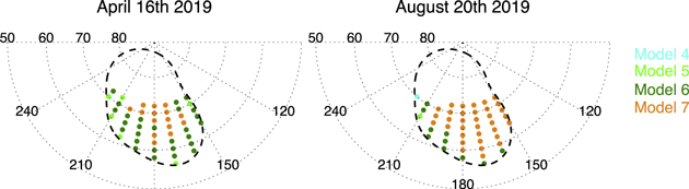
Figure 11. Best-fitting models as a function of latitude and longitude within Jupiter's northern auroral regions, colored according to the legend (and identical to the scheme shown in Figure 2). The results for 2019 April 16 and August 20 are shown in the left and right panels, respectively. Black dashed lines mark the statistical-mean position of the ultraviolet main oval emission (Bonfond et al. 2017). Results outside the main oval are omitted, since they have limited sensitivity when binned by latitude and longitude.
Download figure:
Standard image High-resolution imageOn both dates, the fit to almost all observations within the northern auroral region is optimized using either model 6 or model 7. While there appears to be variability between the 2019 April 16 and August 20 measurements, with model 6 better fitting most locations on the former date and model 7 on the latter, the change in χ2 or the quality of the fit to the spectra is not significant. This is demonstrated in Figure 12, which shows absolute χ2 values for the nine atmospheric models tested in several locations on both dates. Thus, our observations do not indicate any statistically significant spatial variability of the CH4 homopause altitude within the main auroral oval or any temporal variability between 2019 April 16 and August 20. However, given the limits on the sensitivity and spatial resolution of our observations, we cannot rule out such temporal or spatial variability.
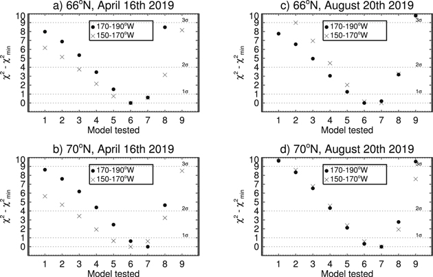
Figure 12. Absolute χ2 values, with respect to the minimum χ2, as a function of atmospheric model tested for different longitude ranges at different latitudes. The top and bottom rows show the results for 66°N and 70°N, respectively, and the left and right columns shown the results for observations recorded on 2019 April 16 and August 20, respectively. Results for observations sampling 170°–190°W (near the center of the main oval) are shown as filled circles, and results for 150°–170°W (dusk side of the main oval) are shown as crosses. Horizontal dashed lines mark the 1σ, 2σ, and 3σ levels in every panel. Only the zero to 3σ range is shown; missing results are outside this range.
Download figure:
Standard image High-resolution image4.5. A Priori Testing
In order to rule out the aforementioned results being an artifact of the chosen a priori temperature profile, we repeated the retrievals of temperature using a set of alternative temperature a priori. This was performed only on the nonauroral longitudinal-mean spectra at 68°N and the spectrum coadded from 68°N, 170°–190°W to assess how the chosen temperature a priori changes the result in each location and relative contrasts between each location. Alternative temperature profiles were computed by moving the base of the thermosphere to higher pressures or shifting the stratospheric isotherm to cooler and warmer temperatures. Figure 13 shows the resulting retrieved temperature profiles and the absolute χ2 fits to the spectra.
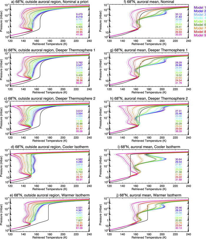
Figure 13. Testing of temperature retrievals from 2019 August 20 measurements with respect to the initial a priori profile assumed. Results for the nonauroral longitudinal-mean spectra at 68°N are shown in the left column and the auroral-mean spectra at 68°N in the right column. The a priori profiles are shown in black, and the solid colored profiles represent the temperature profile retrieved assuming models 1–9, as indicated in the legend. Dotted lines of the same color mark the 1σ retrieval uncertainty. The absolute χ2 fits are shown in each panel with the same color scheme. The first row shows the results assuming the nominal temperature profile as a priori, the second and third rows show the results where the transition to the thermosphere is placed at a higher pressure, and the fourth and fifth rows show the results when a stratospheric isotherm is moved to a cooler and warmer temperature, respectively. Retrieved profiles will tend back to a priori values at pressures where there is no sensitivity in the observations. This gives the appearance of maxima in temperature in the upper stratosphere, which is not physical.
Download figure:
Standard image High-resolution imageFor a given atmospheric model, temperature profiles retrieved from different a priori generally converge on a common profile between approximately 10 mbars and 1 μbar. Outside this pressure range, where there is no information in the spectra, retrieved profiles will tend back to the a priori profile. At 68°N, 170°–190°W, warm stratospheric temperatures are retrieved at approximately the 10 μbar level but then reach a local temperature maximum around the 1–10 μbar level. This is an artifact of the retrieved profile tending back to the a priori; in reality, the warm stratospheric temperatures retrieved at ∼10 μbars denote the base of the thermosphere, which is indeed at a deeper altitude in Jupiter's auroral regions (e.g., Grodent et al. 2001; Bougher et al. 2005; Sinclair et al. 2018).
For the auroral-mean observation at 68°N, using different temperature a priori does yield variation in the atmospheric model that optimizes the fit to the observations; however, the change is within the 1σ confidence levels derived in Section 4.4.1. For example, in using the nominal a priori, adopting the vertical profiles of CH3 and CH4 from model 7 minimizes the absolute χ2 (with a value of 24.29), but model 6 also fits the observations within the 1σ confidence level (χ2 = 24.41). In moving the base of the thermosphere to a lower altitude or the stratospheric isotherm to a cooler temperature, model 6 instead optimizes the fit to the observations. For the nonauroral longitudinal-mean observation at 68°N, there is also a variation in the best-fitting atmospheric model depending on the chosen temperature a priori. However, for a given temperature a priori, the observations inside the main oval are better fit with a higher-altitude CH4 homopause model compared to the observations outside the main oval in the same latitude band.
4.6. Allowing CH3 to Vary
As detailed further in Section 4.1, our retrieval approach thus far has only allowed the vertical temperature profile to vary in order to simultaneously fit the observed H2 S(1) quadrupole and CH3 and CH4 emission. While this has allowed the majority of observations to be modeled within the 1σ level, the core of the CH3 emission was not adequately fit for a subset of observations that directly sampled the auroral regions.
For the auroral-mean observation at 68°N, we performed an additional set of retrievals where models 1–9 were adopted in turn, and the vertical profiles of both temperature and CH3 were allowed to vary. Figure 14 shows the variation in absolute χ2 as a function of model tested when only temperature was allowed to vary and when both temperature and CH3 were allowed to vary. Regardless of whether one or both of temperature and CH3 are allowed to vary, model 6 optimizes the fit to the observations. In allowing both temperature and CH3 to vary, models 1–5 also fit the observations within the 1σ level in absolute χ2. However, we rule out such models as being unphysical. For example, using model 1 requires approximately an order-of-magnitude enhancement in the vertical profile of CH3 to fit its emission feature. As discussed previously in Section 4.1, this would imply the vertical profile of CH4 adopted was also incorrect, which in turn affects the retrieved temperature profile, which in turn affects the vertical profile of CH3, and so on.
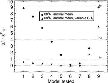
Figure 14. Variations in absolute χ2 in modeling the auroral-mean observation at 68°N when only the vertical temperature was allowed to vary (results shown as circles) and when the vertical profiles of both temperature and CH3 were allowed to vary (results shown as triangles).
Download figure:
Standard image High-resolution imageThe observed and modeled spectra and corresponding retrievals for model 6, when both temperature and CH3 were allowed to vary, are shown in Figure 15. For comparison, the model spectra and temperature profile retrieved when only allowing temperature to vary are also shown. Fitting the CH3 emission feature requires a 3.0 ± 0.7 scale factor increase or a volume mixing ratio increase of (2.04 ± 0.75) × 10−6 in CH3 abundance at 0.33 μbar with respect to the predicted vertical profile of CH3 from model 7. Allowing CH3 to vary has a negligible effect on the quality of the fit to the CH4 emission or the retrieved vertical temperature profile.
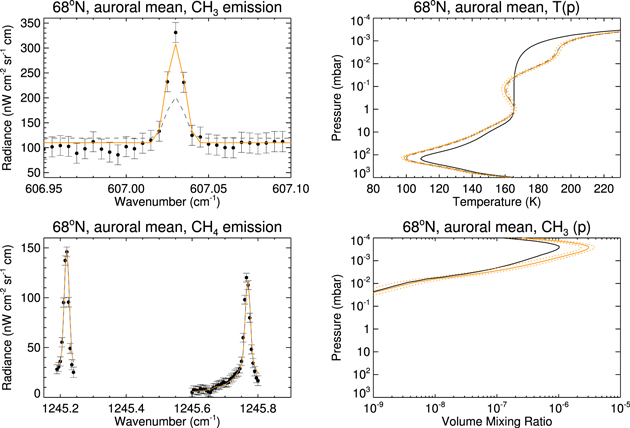
Figure 15. The observed auroral-mean spectra at 68°N (black points with error bars) and modeled spectra (orange solid lines) are shown in the top two panels. The corresponding vertical profiles of temperature and CH3 are shown in the bottom left and bottom right panels, respectively. Black solid lines denote the a priori profile, orange solid lines show the retrieved profile, and orange dotted lines mark the 1σ retrieval uncertainty. For comparison, the model spectra and retrieved temperature profiles, when only temperature is allowed to vary, are shown as gray dashed lines. There is a negligible change in the modeled CH4 emission and temperature profile when only temperature is allowed to vary and when both temperature and CH3 are allowed to vary.
Download figure:
Standard image High-resolution image5. Discussion
At latitudes equatorward of those that include Jupiter's auroral regions, model 1 optimizes the fit to the nonauroral longitudinal-mean observed CH3 and CH4 emission (Section 4.3). For example, at 50°N, we derive a CH4 homopause altitude of 332 km above the 1 bar level, with 357 km marking the upper 1σ confidence level. Since model 1 assumes the lowest-altitude CH4 homopause tested in this work, we cannot derive a lower confidence level. A relatively lower-altitude CH4 homopause at a lower latitude is consistent with Greathouse et al. (2010), who analyzed measurements of a stellar occultation of Jupiter's atmosphere at equatorial latitudes using New Horizons/Alice (Stern et al. 2008). They found that the photochemical named "model C" of Moses et al. (2005), which assumed a lower-altitude CH4 homopause compared to other models presented in the paper, exhibited the best agreement with the observations.
In going poleward of ∼62°S and ∼54°N, the fit to the nonauroral longitudinal-mean observations using model 1 (and other lower-altitude homopause models) deteriorates, and models that adopt a higher-altitude CH4 homopause significantly improve the fit to the observations, particularly to the CH3 emission (Figure 6). For example, at 68°N, sampling only longitudes outside the auroral oval, we derive a homopause altitude of  km. The latitudes at which higher-altitude homopause models provide improved fits are not symmetric in each hemisphere and in fact are well correlated with the latitudinal extent of the southern and northern ovals, once diffraction and the latitudinal binning of the observations are accounted for. This is true even though these observations do not directly sample the longitudes inside the auroral regions. This does suggest a connection with processes related to the aurora, as discussed further below.
We confirm the hypotheses presented in previous studies (e.g., Parkinson et al. 2006; Gustin et al. 2016; Clark et al. 2018) that the CH4 homopause altitude is higher inside Jupiter's main auroral oval compared to elsewhere on the planet. For example, at 62°N, sampling longitudes outside the main oval, we derive a homopause altitude of 331 km with a 1σ upper limit at 370 km. At the same latitude and using a mean spectrum sampling all longitudes inside the main oval, we derive a homopause altitude of  km. Thus, the CH4 homopause altitude is approximately ∼130 km higher inside Jupiter's main auroral oval compared to the atmosphere outside, which is commensurate with the value suggested in Gustin et al. (2016). Our interpretation is that a proportion of energy from the magnetosphere heats the stratosphere within the main oval, which expands the atmosphere and drives vertical winds and/or higher rates of turbulence. This transports CH4 and its photochemical by-products, including CH3, to higher altitudes.
The contrast in CH4 homopause altitude inside and outside the main oval appears to decrease with increasing latitude. For example, at 66°N, we derive a CH4 homopause altitude of  km in sampling longitudes outside the main oval and an altitude of
  km for a mean of longitudes inside the main oval in the same latitude band. Similarly, at 70°N, we derive a homopause altitude of
  km outside the main oval and
  km inside the main oval, which agree within the 1σ level. We believe this can be explained by horizontal transport. Inside the main oval, CH4 is lofted to higher altitudes and subsequently transported to longitudes outside the main oval by horizontal diffusion and advection. Thus, spectra outside the main oval at higher latitudes are also better fit with atmospheric models that have higher abundances of CH4 and its by-products at higher altitudes. Horizontal transport may be more efficient at higher latitudes because of (1) the smaller circumference of a latitude circle at higher latitudes, which allows transport on shorter timescales for a given zonal-wind speed/horizontal diffusion coefficient, and/or (2) higher zonal-wind speeds poleward of 66°N. At least in a longitudinal-mean sense, the meridional increase in temperature at 10 μbars (Figure 6) denotes a wind shear in the zonal direction. From a statistical point of view, there are also fewer individual spectra available to coadd at higher latitudes, which results in higher radiance uncertainties and ultimately higher error bars on derived homopause altitudes.
For observations that sampled longitudes within the main auroral oval, varying the vertical temperature profile alone did not provide adequate fits to the core of the observed CH3 emission. This was improved by allowing the vertical profiles of both temperature and CH3 to vary simultaneously. At 68°N, in order to fit the spectra capturing a mean of all longitudes sampled inside the main oval, a scale factor of 3 increase in CH3 abundance centered at ∼0.3 μbar was required with respect to the CH3 profile predicted in model 6. This increase could be explained by the uncertainties of the chemical model (e.g., Dobrijevic et al. 2003, 2010 further describe the CH3 uncertainties for similar models of Saturn and Neptune). The largest uncertainty in the predicted CH3 mixing ratio in the chemical model (aside from the eddy diffusion coefficient profile) arises from uncertainties in the low-pressure behavior of the reaction CH3 + CH3 + M = C2H6 + M (see the discussion in Bezard et al. 1998; Bézard et al. 1999). Following Moses & Poppe (2017), we have adopted the rate coefficient expression of Vuitton et al. (2012) for this reaction, which includes radiative association, as being the best available literature value. However, we cannot rule out additional sources of CH3 production in Jupiter's auroral regions. This could be in the form of diffuse ultraviolet auroral emissions, in addition to the solar ultraviolet light, which result in a higher rate of CH4 photolysis. Or, currents of energetic ions/electrons could produce higher rates of ion-neutral and electron-recombination reactions, which may also ultimately increase the production of CH3.
Our observations did not demonstrate a statistically significant spatial variation in the CH4 homopause altitude within the northern main auroral oval or any temporal variability between the measurements recorded on 2019 April 16 and August 20. However, this may simply be a result of the limited sensitivity and spatial resolution of the observations. Figure C1 shows predicted solar-wind dynamical pressures at Jupiter during the periods of both measurements on 2019 April 16 and August 20. Appendix C further details the model used to predict solar-wind pressures at Jupiter. The solar wind at Jupiter was relatively quiescent and steady in the days preceding the 2019 April 16 measurements. However, the August 20 measurements were recorded in the 5 days following a series of solar-wind compression arrivals at Jupiter's magnetosphere. While the Jovian magnetosphere is not considered to be open directly to the solar wind, varying external solar-wind conditions can perturb the Jovian magnetosphere through Kelvin–Helmholtz instabilities on the flank and reconnection as part of the Vasiluynas cycle (e.g., Bagenal et al. 2017; Masters 2018; Vogt et al. 2019). Such perturbations can ultimately deposit energy into the neutral atmosphere and modify the morphology and magnitude of the ultraviolet auroral (e.g., Kita et al. 2016; Nichols et al. 2017) and mid-infrared (Sinclair et al. 2019b) emissions. Such variations may be within the sensitivity of TEXES on the IRTF and therefore not observable. We plan to perform similar measurements and analysis using TEXES on Gemini-North. Gemini-North has an 8 m primary aperture, compared to the 3 m primary on the IRTF. This will allow TEXES spectra to be measured with a higher diffraction-limited spatial resolution to better resolve smaller-scale morphology. The smaller plate scale also allows a larger number of spectra to be recorded within a given area on the planet, which allows coadded observations to be computed at a higher S/N.
Our observations on 2019 April 16 and August 20 did not sufficiently sample longitudes inside the southern main oval. Thus, a similar analysis, to determine whether the higher CH4 homopause altitude is isolated in the main oval, could not be performed. Nevertheless, the nonauroral longitudinal-mean observations poleward of 64°S are best fit using models 6–7, even though the southern main oval is not directly sampled by the spectra. This is also suggestive that zonal advection and diffusion can effectively transport CH4 lofted to higher altitudes within the main oval to longitudes outside the main oval. In future observations, we will attempt to better sample the longitudes inside the southern auroral oval and perform a similar analysis.
We note that the results of this study are inconsistent with the results of Kim et al. (2017), who derived a vertical CH4 profile within the northern auroral oval from 3 and 8 μm CH4 emission spectra measured by Gemini/GNIRS and IRTF/TEXES in 2013. Their derived CH4 profile within the northern auroral oval was consistent with that derived from equatorial regions in Kim et al. (2014) using Infrared Space Observatory (ISO) spectra. Inside the northern auroral oval, they derived an upper-limit volume mixing ratio of CH4 of approximately 1 × 10⁻⁴ at the 1 μbar level, which is most consistent with model 1 presented in this study (Figure 2). A possible source of the discrepancy is the uncertainties in the spectroscopic line data of CH4. Indeed, Kim et al. (2020) reanalyzed the 3 μm CH4 emissions in the ISO spectrum, previously presented in Kim et al. (2014), using vibrational–relaxational rates instead assumed from Menard-Bourcin et al. (2005). Their updated vertical profile of CH4 exhibited better agreement with "model C" of Moses et al. (2005) and the analysis of occultation data of Greathouse et al. (2010). A similar reanalysis of the 3 μm CH4 emissions presented in Kim et al. (2017) of the northern auroral hot spot may also improve the agreement of our study and Kim et al. (2017). Further sources of inconsistency include the relatively larger nonthermal contribution in the 3 μm CH4 emissions compared to the 8 μm emissions in this study and/or temporal variability between the observations measured in 2013 in their study and the 2019 observations in this study. The potential for temporal variability could be explored by repeating measurements on further dates. Although the results from measurements on 2019 April 16 and August 20 appear similar, we cannot rule out temporal variability outside of those dates. Sinclair et al. (2019b) demonstrated daily variability of the 8 μm CH4 emissions, which was possibly triggered by a solar-wind compression that perturbed the magnetosphere.
We note for readers one limitation of our analysis: the assumption of LTE in the NEMESIS radiative transfer code. The assumption of "classical" LTE requires a sufficient number of intermolecular collisions such that the energy populations of a molecule's translational, vibrational, and rotational states remain in equilibrium (López-Puertas & Taylor 2001). This allows the population of states of the rotational and vibrational modes to be calculated using the Boltzmann equation; thus, the source function is the Planck function (blackbody). However, at lower atmospheric pressures, the frequency of intermolecular collisions drops such that the assumption of LTE is less valid with increasing altitude/decreasing pressure (e.g., Appleby 1990; López-Puertas & Taylor 2001). As a result, the source function departs from a blackbody. Figure D1 shows the source function–to–Planck function ratios as a function of pressure for Jupiter's hydrocarbons, including CH4 and CH3. Appendix D further details the non-LTE calculation used to derive these source functions. The source function of CH4 begins to deviate from a blackbody at approximately 1 mbar but remains in LTE to a greater extent than its photochemical by-products at pressures lower than ∼3 μbars. The source functions of CH3 and higher-order hydrocarbons depart from LTE at approximately 0.1 mbar or 190 km above the 1 bar level. Thus, in the upper stratosphere, both CH3 and CH4, and particularly CH3, will produce less emission in their respective emission features at 607.03 and 1245–1252 cm−1 than if the atmosphere was in LTE. NEMESIS assumes the atmosphere is in LTE and thus will interpret the lower observed emission as either cooler temperatures in the line-forming region of each species and/or a lower-altitude CH4 homopause that places less CH4 and CH3 at higher altitudes. Therefore, we hypothesize that the assumption of LTE in our radiative transfer code may result in underestimated atmospheric temperatures at high altitudes and/or underestimated CH4 homopause altitudes. However, the effect of non-LTE in our analysis can only be quantified with a radiative transfer code that self-consistently parameterizes non-blackbody source functions. This will be the subject of future work. In the meantime, absolute temperatures or homopause altitudes should be treated with caution. However, to first order, we believe relative variations can be spatially/temporarily interpreted at face value.
6. Conclusions
We performed an analysis of IRTF-TEXES high-resolution spectra of Jupiter's mid-to-high-latitude H2 S(1), CH3, and CH4 emission recorded on 2019 April 16 and August 20. The spectra were inverted to constrain the height of the CH4 homopause and its spatial variation across the planet. A family of photochemical models, based on Moses & Poppe (2017), was computed by varying the eddy diffusion coefficient profile in the upper stratosphere and thereby increasing the altitude of the CH4 homopause and lofting CH3 and CH4 to higher altitudes. Adopting each photochemical model in turn, the emission features of H2 S(1), CH3, and CH4 were modeled simultaneously by allowing the vertical temperature profile to vary, and the quality of the fit to the observed CH3 and CH4 emission was used to discriminate between models. At latitudes equatorward of those that include Jupiter's main auroral ovals (>62°S, <54°N, planetocentric), the fit to the observations was optimized using a photochemical model, which assumed the lowest-altitude CH4 homopause tested. At 50°N, we derive a CH4 homopause altitude of 332 km above the 1 bar level, with a 1σ upper limit of 357 km. At higher latitudes, we confirm the hypothesis presented in previous work (e.g., Parkinson et al. 2006; Gustin et al. 2016; Clark et al. 2018) that the CH4 homopause is higher in altitude in Jupiter's auroral regions compared to elsewhere on the planet. For example, at 62°N, sampling longitudes inside the main auroral oval, we derive a CH4 homopause altitude of  km. This is in contrast to an altitude of 331 km, with a 1σ upper limit at 370 km, derived for longitudes outside the main auroral oval in the same latitude band. Our interpretation is that a proportion of energy from the magnetosphere is deposited in the form of heat within the main oval, which drives vertical winds and/or higher rates of turbulence and transports CH4 and its photochemical by-products to higher altitudes. Observations inside the northern main auroral oval also required a factor of ∼3 enhancement in CH3 in order to best fit the core of the CH3 emission feature within the 1σ noise. This is partly explained by uncertainties in the photochemical modeling. It could also be suggestive of an additional source of CH3 production in Jupiter's auroral regions compared to elsewhere on the planet, possibly due to diffuse ultraviolet auroral emissions or ion-neutral chemistry due to currents of energetic charged particles. We note to readers that our analysis assumed LTE, whereas the upper stratosphere studied in this work may have departed significantly from LTE conditions. Thus, absolute retrieved temperatures, abundances, and homopause altitudes should be interpreted with caution. However, we expect relative spatial or temporal variations to be robust.
The research was carried out at the Jet Propulsion Laboratory, California Institute of Technology, under a contract with the National Aeronautics and Space Administration (NASA). The material is based upon work supported by NASA under grant NNH17ZDA001N issued through the Solar System Observations Planetary Astronomy program. The observations were recorded by T.K.G., R.S.G., and A.A. as Visiting Astronomers at NASA's Infrared Telescope Facility (IRTF) under grant 80HQTR19D0030. The IRTF is operated by the University of Hawaii under contract NNH14CK55B with NASA. J.I.M. acknowledges support from NASA Solar System Workings program 80NSSC20K0462. L.N.F. was supported by a Royal Society Research Fellowship and European Research Council Consolidator grant (under the European Union's Horizon 2020 research and innovation program, grant agreement No. 723890) at the University of Leicester. Coinvestigator C.T. acknowledges support by MEXT/JSPS KAKENHI grant 19H01948.
Software: NEMESIS (Irwin et al. 2008), FUTBOLIN (Martín-Torres & Mlynczak 2005).
Appendix A: Observation Details
Tables A1 and A2 provide details of the observations recorded on 2019 April 16 and August 20.
Table A1. Details of the Spectra Measured on 2019 April 16
| Date | Time | File Name | Setting | Number | Airmass | Hemisphere | Median |
|---|---|---|---|---|---|---|---|
| of Spectra | Longitude | ||||||
| 2019 Apr 16 | 11:14:54 | jup.2010.01 | 1248 | 927 | 2.12000 | N | 114 |
| 11:14:54 | jup.2010.02 | 1248 | 669 | 2.12000 | N | 115 | |
| 11:20:48 | jup.2011.01 | 1248 | 437 | 2.05000 | N | 116 | |
| 11:26:18 | jup.2012.01 | 1248 | 420 | 1.99000 | N | 119 | |
| 11:29:26 | jup.2013.01 | 1248 | 850 | 1.96000 | S | 127 | |
| 11:29:26 | jup.2013.02 | 1248 | 408 | 1.96000 | S | 131 | |
| 11:36:28 | jup.2014.01 | 587 | 953 | 1.89000 | N | 127 | |
| 11:39:42 | jup.2015.01 | 587 | 615 | 1.86000 | N | 128 | |
| 11:39:42 | jup.2015.02 | 587 | 705 | 1.86000 | N | 130 | |
| 11:45:18 | jup.2016.01 | 587 | 592 | 1.82000 | S | 138 | |
| 11:45:18 | jup.2016.02 | 587 | 518 | 1.82000 | S | 140 | |
| 11:52:16 | jup.2017.02 | 607 | 959 | 1.76000 | N | 139 | |
| 12:00:07 | jup.2018.01 | 607 | 639 | 1.71000 | N | 140 | |
| 12:00:07 | jup.2018.02 | 607 | 773 | 1.71000 | N | 143 | |
| 12:08:15 | jup.2019.01 | 607 | 324 | 1.66000 | S | 154 | |
| 12:08:15 | jup.2019.02 | 607 | 435 | 1.66000 | S | 155 | |
| 13:10:29 | jup.2028.01 | 1248 | 509 | 1.43000 | N | 183 | |
| 13:10:29 | jup.2028.02 | 1248 | 160 | 1.43000 | N | 182 | |
| 13:15:59 | jup.2029.01 | 1248 | 576 | 1.41000 | S | 193 | |
| 13:15:59 | jup.2029.02 | 1248 | 238 | 1.41000 | S | 196 | |
| 13:23:27 | jup.2030.01 | 587 | 867 | 1.40000 | N | 191 | |
| 13:23:27 | jup.2030.02 | 587 | 561 | 1.40000 | N | 192 | |
| 13:28:55 | jup.2031.01 | 587 | 457 | 1.39000 | S | 200 | |
| 13:28:55 | jup.2031.02 | 587 | 398 | 1.39000 | S | 203 | |
| 13:35:58 | jup.2032.01 | 607 | 397 | 1.38000 | N | 198 | |
| 13:35:58 | jup.2032.02 | 607 | 456 | 1.38000 | N | 200 | |
| 13:43:48 | jup.2033.01 | 607 | 514 | 1.37000 | S | 210 | |
| 13:43:48 | jup.2033.02 | 607 | 495 | 1.37000 | S | 212 | |
| 14:46:27 | jup.2042.01 | 1248 | 578 | 1.36000 | N | 241 | |
| 14:49:46 | jup.2043.01 | 1248 | 606 | 1.36000 | N | 243 | |
| 14:49:46 | jup.2043.02 | 1248 | 303 | 1.36000 | N | 244 | |
| 14:55:18 | jup.2044.01 | 1248 | 442 | 1.37000 | S | 253 | |
| 14:55:18 | jup.2044.02 | 1248 | 215 | 1.37000 | S | 257 | |
| 15:02:42 | jup.2045.01 | 587 | 671 | 1.38000 | N | 250 | |
| 15:02:42 | jup.2045.02 | 587 | 684 | 1.38000 | N | 252 | |
| 15:08:16 | jup.2046.01 | 587 | 356 | 1.39000 | S | 263 | |
| 15:15:30 | jup.2047.01 | 607 | 474 | 1.40000 | N | 259 | |
| 15:15:30 | jup.2047.02 | 607 | 474 | 1.40000 | N | 262 | |
| 15:27:15 | jup.2048.01 | 607 | 639 | 1.42000 | S | 272 | |
| 15:27:15 | jup.2048.02 | 607 | 435 | 1.42000 | S | 275 | |
| 16:26:57 | jup.2056.01 | 1248 | 357 | 1.64000 | N | 295 | |
| 16:26:57 | jup.2056.02 | 1248 | 172 | 1.64000 | N | 296 | |
| 16:32:37 | jup.2057.01 | 1248 | 689 | 1.68000 | S | 294 | |
| 16:32:37 | jup.2057.02 | 1248 | 563 | 1.68000 | S | 294 | |
| 16:40:44 | jup.2058.01 | 587 | 217 | 1.73000 | N | 300 | |
| 16:40:44 | jup.2058.02 | 587 | 268 | 1.73000 | N | 300 | |
| 16:46:17 | jup.2059.01 | 587 | 1039 | 1.77000 | S | 295 | |
| 16:46:17 | jup.2059.02 | 587 | 858 | 1.77000 | S | 296 |
Note. All dates/times are UTC.
Download table as: ASCIITypeset image
Table A2. Details of the Spectra Measured on 2019 August 20
| Date | Time | File Name | Setting | Number | Airmass | Hemisphere | Median |
|---|---|---|---|---|---|---|---|
| of Spectra | Longitude | ||||||
| 2019 Aug 20 | 02:39:10 | jup.8001.01 | 1248 | 602 | 1.87000 | N | 59 |
| 02:39:10 | jup.8001.02 | 1248 | 519 | 1.87000 | N | 58 | |
| 02:39:10 | jup.8001.03 | 1248 | 476 | 1.87000 | N | 59 | |
| 02:47:01 | jup.8002.01 | 1248 | 263 | 1.81000 | S | 87 | |
| 02:47:01 | jup.8002.02 | 1248 | 240 | 1.81000 | S | 87 | |
| 02:54:09 | jup.8003.01 | 587 | 764 | 1.76000 | N | 63 | |
| 02:54:09 | jup.8003.02 | 587 | 672 | 1.76000 | N | 64 | |
| 02:54:09 | jup.8003.03 | 587 | 811 | 1.76000 | N | 65 | |
| 03:01:47 | jup.8004.01 | 587 | 632 | 1.70000 | S | 89 | |
| 03:01:47 | jup.8004.02 | 587 | 767 | 1.70000 | S | 89 | |
| 03:24:27 | jup.8007.01 | 607 | 272 | 1.58000 | S | 107 | |
| 03:24:27 | jup.8007.02 | 607 | 417 | 1.58000 | S | 105 | |
| 03:24:27 | jup.8007.03 | 607 | 414 | 1.58000 | S | 107 | |
| 03:35:50 | jup.8008.01 | 607 | 539 | 1.53000 | N | 84 | |
| 03:35:50 | jup.8008.02 | 607 | 765 | 1.53000 | N | 88 | |
| 04:40:27 | jup.8017.01 | 1248 | 499 | 1.37000 | N | 123 | |
| 04:40:27 | jup.8017.02 | 1248 | 320 | 1.37000 | N | 124 | |
| 04:40:27 | jup.8017.03 | 1248 | 398 | 1.37000 | N | 127 | |
| 04:48:08 | jup.8018.01 | 1248 | 390 | 1.36000 | S | 152 | |
| 04:48:08 | jup.8018.02 | 1248 | 240 | 1.36000 | S | 157 | |
| 04:55:08 | jup.8019.01 | 587 | 457 | 1.35000 | S | 156 | |
| 04:55:08 | jup.8019.02 | 587 | 736 | 1.35000 | S | 155 | |
| 05:00:30 | jup.8020.01 | 587 | 702 | 1.35000 | N | 136 | |
| 05:00:30 | jup.8020.02 | 587 | 725 | 1.35000 | N | 138 | |
| 05:07:17 | jup.8021.01 | 607 | 829 | 1.34000 | N | 141 | |
| 05:07:17 | jup.8021.02 | 607 | 549 | 1.34000 | N | 142 | |
| 05:07:17 | jup.8021.03 | 607 | 629 | 1.34000 | N | 145 | |
| 05:18:37 | jup.8022.01 | 607 | 552 | 1.34000 | S | 170 | |
| 05:18:37 | jup.8022.02 | 607 | 484 | 1.34000 | S | 173 | |
| 06:18:45 | jup.8031.01 | 1248 | 423 | 1.39000 | N | 182 | |
| 06:18:45 | jup.8031.02 | 1248 | 322 | 1.39000 | N | 182 | |
| 06:24:13 | jup.8032.01 | 1248 | 462 | 1.40000 | S | 209 | |
| 06:24:13 | jup.8032.02 | 1248 | 422 | 1.40000 | S | 211 | |
| 06:31:35 | jup.8033.01 | 587 | 589 | 1.42000 | N | 191 | |
| 06:31:35 | jup.8033.02 | 587 | 736 | 1.42000 | N | 193 | |
| 06:31:35 | jup.8033.03 | 587 | 723 | 1.42000 | N | 195 | |
| 06:39:18 | jup.8034.01 | 587 | 689 | 1.43000 | S | 217 | |
| 06:39:18 | jup.8034.02 | 587 | 810 | 1.43000 | S | 218 | |
| 06:46:09 | jup.8035.01 | 607 | 519 | 1.45000 | N | 199 | |
| 06:46:09 | jup.8035.02 | 607 | 610 | 1.45000 | N | 203 | |
| 06:54:02 | jup.8036.01 | 607 | 600 | 1.48000 | S | 227 | |
| 06:54:02 | jup.8036.02 | 607 | 690 | 1.48000 | S | 229 |
Note. All dates/times are UTC.
Download table as: ASCIITypeset image
Appendix B: 2019 April 16 Results
Figure B1 shows the results of temperature retrievals from nonauroral longitudinal-mean spectra recorded on 2019 April 16.

Figure B1. Longitudinal-mean retrievals of temperature as a function of latitude at mid-to-high southern (left column) and northern (right column) latitudes. The results are colored according to the model profiles of CH3 and CH4 adopted (and identical to the color scheme shown in Figure 2). Temperatures at 0.01, 0.1, and 1.0 mbar are shown in the first, second, and third rows, respectively. The fourth, fifth, and sixth rows show the reduced χ2 fit to the CH3 emission feature from 607.01 to 607.05 cm−1, all sampled CH4 emission from 1245.19 to 1250.05 cm−1, and the combined fit to the CH3 and CH4 emission, respectively. In all panels, the vertical dashed lines mark the lowest-latitude extent of the ultraviolet main auroral ovals (Bonfond et al. 2017).
Download figure:
Standard image High-resolution imageAppendix C: Solar-wind Conditions
The solar-wind dynamical pressure (pdyn = ρv2, where ρ is the density and v is the velocity of the solar wind) impinging on Jupiter's magnetosphere was calculated using a solar-wind propagation model (Tao et al. 2005). This model is used extensively by the outer planets' magnetosphere community in the absence of in situ measurements of the solar-wind conditions (e.g., Badman et al. 2016; Kinrade et al. 2017; Lamy et al. 2017). The model adopts hourly measurements of the solar wind and magnetic field at Earth's bow-shock nose from OMNI (Thatcher & Müller 2011) and then performs 1D magnetohydrodynamic (MHD) calculations to model the solar-wind flow out to Jupiter's bow shock. The 1D nature of the model can introduce uncertainties on the arrival time and magnitude of dynamical pressure of the solar wind. When the Earth–Sun–Jupiter angle is less than ±50° (or when Jupiter is within ∼50 days of opposition), the uncertainty of the arrival time of the solar-wind shock is less than ±20 hr, and that of the maximum dynamic pressure is 38% (Zieger & Hansen 2008; Kita et al. 2016). For Earth–Sun–Jupiter angles, the error on timing can be as high as 48 hr (Sinclair et al. 2019b).
Figure C1 shows the predicted solar-wind conditions during the periods when the TEXES measurements analyzed in this study were recorded. The 2019 April 16 measurements were recorded during a period of quiescent, steady solar-wind conditions with a <0.2 nPa solar-wind compression on 2019 April 13. However, the Earth–Sun–Jupiter angle was larger than 60° during this period; thus, the timing of solar-wind events could be offset by as much as 48 hr. The August 20 measurements were recorded during a period of varying solar-wind conditions with a strong (∼0.37 nPa) solar-wind compression recorded late on 2019 August 13.
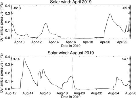
Figure C1. Predicted solar-wind dynamical pressure at Jupiter in 2019 April (top) and August (bottom). The vertical dashed lines mark the mean dates/times of the observations analyzed in this study. The Earth–Sun–Jupiter angle is shown in the top left and right of each panel. Model timing and dynamical pressures are most accurate when Jupiter is within 60° of opposition.
Download figure:
Standard image High-resolution imageAppendix D: Non-LTE
Figure D1 shows the source function–to–Planck function ratios (henceforth abbreviated to J/B) of the mid-infrared bands of CH3, CH4, C2H2, C2H4, C2H6, CH3C2, C4H2, and C6H6 on Jupiter. The J/B profiles are generally used to quantify the departure of LTE for a given molecule as a function of pressure or altitude. These were calculated using an updated version of the non-LTE model used in Martín-Torres et al. (1998) and Orton et al. (2014a, 2014b). The calculation assumed the vertical profiles of temperature and all aforementioned hydrocarbons from model 1, a latitude of 62°N was assumed, and the pressure–altitude grid was calculated assuming hydrostatic equilibrium. The non-LTE model includes the calculation of the vibrational excitation of CH4 and the hydrocarbons CH3, C2H6, C2H2, and C2H4. The model includes exchanges of energy in vibrational–translational (V–T) and vibrational–vibrational (V–V) processes, as well as by radiative processes. The radiative and collisional productions and losses are combined in a number of statistical equilibrium equations for each vibrational level. Radiative processes include spontaneous emission, direct absorption of solar radiation, and the exchange of photons among the atmospheric layers. The exchange between layers is treated using the Full transfer by Optimized LINe-by-line (FUTBOLIN) radiative transfer code (Kratz et al. 2005; Martín-Torres & Mlynczak 2005). The current version of the model assumes the CH4 collisional rates from Martín-Torres & Mlynczak (2005) and the relaxation rates for CH4–H2 from Hess & Moore (1976) and Menard-Bourcin et al. (2000, 2001, 2005). For the collisional rates of the remaining aforementioned hydrocarbons, the formalisms presented in Yelle (1991) were adopted. The model calculation neglects stimulated emission and scattering, which is valid given the atmospheric temperatures and the wavelengths of the transitions considered for these species. A further assumption of the model is that the rotational levels in each vibrational–rotational band are in LTE. The model calculation of level populations described above assumes stationary atmospheric conditions. Further processes in Jupiter's auroral regions, such as proton/electron precipitation, may further deviate the excited states of a molecule population from a Boltzmann population and therefore can also be considered "non-LTE" processes. Such processes are highly time variable and thus have not been included in our calculation of the source functions for the sake of simplicity.
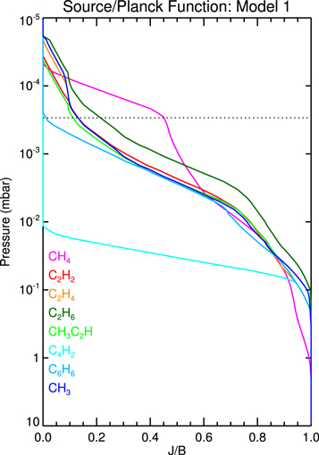
Figure D1. Source function–to–Planck function ratios (J/B) as a function of pressure adopting the vertical profiles of temperature and hydrocarbons from model 1 (Moses & Poppe 2017). The J/B profiles are shown for CH4 (pink), C2H2 (red), C2H4 (orange), C2H6 (dark green), CH3C2H (light green), C4H2 (cyan), C6H6 (light blue), and CH3 (dark blue). The pressure level of the homopause is marked with a horizontal dashed line.
Download figure:
Standard image High-resolution image
For almost all hydrocarbons, the source functions deviate from a blackbody at approximately 0.1 mbar or ∼190 km above the 1 bar level. The exception is CH4, whose source function deviates from a blackbody at approximately 1 mbar but remains in LTE to a greater extent than its photochemical by-products at pressures lower than 1 μbar. The C4H2 deviates from LTE a higher rate with altitude compared to the other species shown. This is due to a combination of V–V coupling with the other species, lower V–T collisional rates, and stronger solar absorption at short wavelengths.