


Abstract
Bulk chemical composition is a fundamental property of a planetary material, rock or regolith, and can be used to constrain the properties and history of a material, and by extension its parent body, including its potential for habitability. Here, we investigate how uncertainties in bulk major element analyses can affect inferences derived from those analyses, including rock classification by total-alkalis–silica (TAS); Chemical Index of Alteration (CIA); a tectonic discriminant for magma genesis; and the inferred mantle pressure and temperature of a basaltic magma's origin. Uncertainties for actual spacecraft instruments (Mars Exploration Rover and Mars Science Laboratory (MER/MSL), Alpha Proton X-Ray Spectroscopy (APXS), and Mars Science Laboratory: Laser-Induced Breakdown Spectroscopy (MSL LIBS)) and a suggested uncertainty level for analyses on Venus (Venus Exploration Targets (VExT) Workshop) are higher than those of standard Earth-based analyses (e.g., by inductively coupled plasma optical emission spectrometry (ICPOES)). We propagate the uncertainties from each analysis type to the derived parameters, both implicitly and via boot-strap (Monte Carlo) methods. Our calculations show that the uncertainties of APXS and VExT are greater than those for ICPOES, but they still allow useful inferences about rock type and history. Our results show that the uncertainties of MSL LIBS analyses are significantly larger than the other techniques, and can provide only limited constraints on rock types or histories. Any instruments chosen for future mission must have uncertainties of the chemical analyses small enough to meet the mission's overall scientific objectives.
Export citation and abstract BibTeX RIS

Original content from this work may be used under the terms of the Creative Commons Attribution 4.0 licence. Any further distribution of this work must maintain attribution to the author(s) and the title of the work, journal citation and DOI.
1. Introduction
The broad objective of major and minor element chemical analyses by landed spacecraft is clear: elemental composition is a fundamental property of a material and can be used in myriad ways to determine the analyzed material's properties and history, and by extension, those of its parent planetary body, including its potential for habitability. However, the goals of such elemental chemical analyses on a spacecraft mission are commonly poorly defined. For example, basalts are abundant on the surfaces of the inner planets (and several asteroids), but what specific questions about a basalt's chemical composition need to be answered, and to what levels of accuracy and precision? Is it crucial merely to know if they are basalts, as opposed to granites or to undifferentiated chondritic material, or is it important to know what broad types of basalt are present (e.g., tholeiitic versus alkaline)? Or perhaps is the mission's goal to constrain the mineralogy and mantle conditions of basalt generation? Without clearly defined goals, it is not possible to know if chemical analytical instrumentation can achieve the goals. Therefore, we explore how uncertainties in major element chemical analyses can affect the ability to discriminate different classes of igneous rocks, chemical weathering, and finally magma genesis conditions (tectonic setting or P–T of magma origin).
Major and minor elements in igneous rocks are those considered to be essential structural elements in most igneous minerals and therefore they make up the majority of igneous rocks (and by extension planetary crusts). These include: SiO2, TiO2, Al2O3, Cr2O3, FeO (and/or Fe2O3), MnO, MgO, CaO, Na2O, K2O, P2O5, and SO3. Other elements (as oxides or not) may be abundant in specific rock types, and therefore can be considered major elements in such rocks: carbon (C) in coal and some sediments, carbon dioxide (CO2) in carbonate rocks, and water (H2O) in rocks rich in clay minerals and some sulfate minerals. These elements and element oxides can represent nearly all of the bulk chemical compositions of solids in the solar system, except those with abundant iron metal; abundant ices, organics, and ammonia compounds, like comets, the outer planets, and their moons; abundant chlorine, like some Mars surface materials; and those that are extremely reduced (like the enstatite meteorites), in which much of their Fe, Mn, Cr, Na, and K reside in sulfide and phosphide minerals.
The science return from the bulk major and minor element chemistry of rocks on other planetary bodies can be huge, and it can be used to constrain a first-order understanding of planetary processes, vis. Janoušek et al. (2015). The sizes of analytical instruments have decreased significantly in the last 60 years (Johnson et al. 2013), as their analytical precisions and accuracies have improved. Only some of these advances have become, or could be, imported to spacecraft instrumentation. For instance, laser-ablation inductively coupled mass spectrometry (LA-ICP-MS) has become a standard method for mineral chemical analyses in Earth laboratories, but it has so far been precluded from spaceflight because of constraints on mass, power, sample preparation, and ruggedness. Therefore, sample return and analyses of meteorites in terrestrial laboratories is still the gold standard. However, much can be done by remote analyses, either based on orbital analyses or in situ from rovers.
The goal of this work is to explore the effects of analytical uncertainties, precision and accuracy, on geochemical and petrologic inferences from chemical analyses of planetary materials. We focus on standard "major element" analyses of basaltic compositions, and calculate constraints including igneous rock classification, degree of weathering, tectonic setting of magma genesis, and pressures and temperatures of magmatic formation. This manuscript is an expansion of work presented in abstract form by Treiman & Dyar (2015) and Treiman & Filiberto (2016), and follows in the footsteps of earlier works by Kring et al. (1995) and Sharpton et al. (2014).
2. Input Data, Computational Methods
2.1. Chemical Compositions
Humphrey. The basalt sample Humphrey was among the first targets analyzed by the Mars Exploration Rover (MER) Spirit in Gusev Crater, Mars and, based on spectral analyses, it is similar in bulk chemistry and mineralogy to much of the lava flow on which Spirit landed–the Adirondack-class basalts (e.g., McSween et al. 2006). The chemical composition of surface, before and after being abraded, was obtained by Alpha Proton X-Ray Spectroscopy (APXS; see Table 1), and is consistent with a terrestrial olivine-tholeiitic basalt (Gellert et al. 2006; McSween et al. 2006; Filiberto et al. 2008). Consistent with its bulk composition, Humphrey's mineralogy includes olivine of intermediate composition, low-Ca pyroxene, and magnetite (e.g., McSween et al. 2006). Extensive experimental and modeling work has used this composition to understand the Martian interior and has shown it represents a fractionated magma composition (Monders et al. 2007; Hausrath et al. 2008; Filiberto et al. 2009; Filiberto & Treiman 2009; Schmidt & McCoy 2010; Stanley et al. 2011; Filiberto & Dasgupta 2011; Filiberto et al. 2014; Udry et al. 2014).
Table 1. Chemical Compositions of Rocks Used Here
| Gusev Basalt | Gale Mudstone | Gale Mudstone | |
|---|---|---|---|
| Humphreya | Marimba 2b | Marimba 2c | |
| SiO2 | 46.96 | 45.99 | 50.99 |
| TiO2 | 0.56 | 1.07 | 0.91 |
| Al2O3 | 10.93 | 8.49 | 9.26 |
| Cr2O3 | 0.64 | 0.33 | ⋯ |
| FeO | 19.23 | 22.53 | 20.08 |
| MnO | 0.42 | 0.09 | ⋯ |
| MgO | 10.65 | 4.58 | 4.57 |
| CaO | 8.02 | 5.27 | 2.97 |
| Na2O | 2.56 | 2.11 | 2.06 |
| K2O | 0.10 | 0.83 | 1.04 |
| P2O5 | 0.57 | 1.05 | ⋯ |
| SO3 | 0.00 | 6.87 | ⋯ |
| Cl | 0 | 0.48 | ⋯ |
| Total | 100.64 | 99.69 | 91.87 |
Notes.
aAnalysis by APXS Gellert et al. (2006). bAnalysis by APXS (Thompson et al. 2020). cAnalysis by LIBS, average of all LIBS shots for drill hole and tailings, from NASA PDS data repository.Download table as: ASCIITypeset image
Marimba. Marimba 2 is a representative sample of the Murray mudstone in Gale Crater, Mars. It was analyzed extensively by the Mars Science Laboratory (MSL) Curiosity rover in its sols 1424–1437, including multiple APXS and Laser-Induced Breakdown Spectroscopy (LIBS) chemical analyses (Table 1), a significance analysis of microarrays (SAM) analysis of its volatile components, and a CheMin X-ray diffraction determination of its mineral abundances (Stern et al. 2017; Bristow et al. 2018; Archer et al. 2019; Mangold et al. 2019; Thompson et al. 2020). The mineralogy of Marimba 2 is consistent with extensive aqueous alteration: ∼30% (by weight) clay minerals (Mg-rich di- and tri-octahedral smectites), ∼40% amorphous material, 6.5% hematite, and ∼7% calcium sulfate; the remainder of the rock is feldspar and pyroxene, inferred to be in original sedimentary grains (Bristow et al. 2018).
2.2. Analytical Methods and their Uncertainties
Many analytical techniques have been used to obtain bulk chemical analyses of rock and other geological materials, but many are unsuitable for spacecraft missions (like wet chemistry) or cannot provide abundances of the ten most common element oxides (like neutron activation gamma-ray spectrometry). While orbital measurements of planetary crusts through neutron activation and gamma-ray spectrometry provide important constraints on the chemical composition and diversity of compositions within a planetary crust including mapping water (e.g., Boynton et al. 2002; Gillis et al. 2004; Taylor et al. 2010a; Prettyman et al. 2012; Williams et al. 2018), these measurements have large spot size (e.g., up to 1 km for Mars) and cannot detect or quantify abundances of important elements (e.g., Mg, Na, and other major elements for Mars, e.g., Boynton et al. 2004; Taylor et al. 2010b). Therefore, here we focus on those techniques that have flown (APXS, LIBS), standard terrestrial rock analyses (inductively coupled plasma optical emission spectrometry (ICPOES)), and target analyses goals for an in situ Venus mission. On Earth, samples are fully processed before analyses, removing all alteration products, dust and other coatings, and fully homogenizing the samples, which provides an accurate analysis of each rock; however, such a process cannot be conducted on another planet and all analyses will include some amount of secondary processing. While we acknowledge this issue, we focus on the accuracy and precision of the instruments themselves and do not quantify the effect of secondary processes on the precision and accuracy of analyses, which would have to be done on a case by case basis (e.g., Schmidt et al. 2018; Berger et al. 2020; Flannigan et al. 2020).
ICPOES. On Earth, ICPOES has become a method of choice for major and minor element analyses, e.g., (Bengtson 2019). In ICPOES, a clean rock sample is dissolved into solution, and the solution ionized to a plasma. Elements in the solutions yield specific ions and interactions in the plasma that emit light, and element abundances are quantified by comparing the strengths of those emissions with emissions from standards. Our estimates of the accuracy and precision of modern bulk-rock ICPOES analyses are from a recent paper, Ciborowski et al. (2015), which examined the geochemistry of basalts from a Proterozoic large igneous province and was particularly clear about the precision and accuracy of their analyses.
APXS. APXS instruments have flown on many spacecraft, going back to the Surveyor 5 lunar lander (Jaffe et al. 1968). On Mars, APXS instruments have operated successfully on the Mars Pathfinder, MER, and MSL rovers (Rieder et al. 1997, 2003; Gellert et al. 2006; Campbell et al. 2012, 2014; Stolper et al. 2013). APXS combines the utility of X-ray fluorescence analysis (XRF), e.g., Sitko & Zawisza (2012), for elements with atomic numbers above 13 or so with the proton excitation's greater X-ray yield lighter elements. Gellert et al. (2006) gives analytical accuracies of the MER APXS instruments (see Table 2); accuracies of the MSL APXS have not been published, but the MER values are inferred to apply (Campbell et al. 2014). APXS precision is based on counting statistics (which are dependent on duration and temperature) for X-ray peaks and a practical fit to the X-ray background; values in Table 2 are from MSL mission "quicklook products," see O'Connell-Cooper et al. (2017), and Thompson et al. (2020).
Table 2. Absolute Uncertainties in Oxide Abundances, Weight %, 1σ
| ICPOESa | APXSb | VExTc | LIBSd | |||||
|---|---|---|---|---|---|---|---|---|
| Uncertainty% | Total | Accuracye | Precision | Total | Total | Accuracy | Precision | Total |
| SiO2 | 0.35 | 1.48 | 0.27 | 1.50 | 2.00 | 5.10 | 0.53 | 5.13 |
| TiO2 | 0.02 | 0.18 | 0.015 | 0.18 | 0.15 | 0.49 | 0.05 | 0.49 |
| Al2O3 | 0.56 | 0.56 | 0.095 | 0.57 | 1.00 | 3.57 | 0.68 | 3.63 |
| Cr2O3 | 2.5 | 0.05 | 0.005 | 0.05 | 0.20 | ⋯ | ⋯ | 0.01 |
| FeO | 0.18 | 1.01 | 0.13 | 1.02 | 0.50 | 3.77 | 0.39 | 3.79 |
| MnO | 0.01 | 0.00 | 0.005 | 0.01 | 0.10 | ⋯ | ⋯ | 0.01 |
| MgO | 0.15 | 0.53 | 0.085 | 0.54 | 0.50 | 1.83 | 0.19 | 1.84 |
| CaO | 0.52 | 0.26 | 0.03 | 0.26 | 0.80 | 2.20 | 0.30 | 2.22 |
| Na2O | 0.21 | 0.07 | 0.035 | 0.08 | 0.20 | 1.00 | 0.25 | 1.03 |
| K2O | 0.04 | 0.07 | 0.02 | 0.08 | 0.05 | 0.62 | 0.15 | 0.64 |
| P2O5 | 0.01 | 0.18 | 0.025 | 0.18 | 0.10 | ⋯ | ⋯ | 0.00 |
| SO3 | 0.01 | 1.29 | 0.035 | 1.29 | 0.30 | ⋯ | ⋯ | 0.00 |
| Cl | 0.01 | 0.09 | 0.01 | 0.09 | 0.10 | ⋯ | ⋯ | 0.00 |
Notes.
aCiborowski et al. (2015), Electronic Annex 1 based on 10 replicates of JB1a standard. Uncertainty for SO3 taken as that for P2O5. bAccuracy from % deviation of element abundances in Table 1 of Gellert et al. (2006), taken as 2σ. These % deviations are applied to the Marimba 2 analysis (Table 1) to give the absolute % uncertainty. Precisions of the Marimba 2 analyses are from O'Connell-Cooper et al. (2017) and Thompson et al. (2020). cFrom Sharpton et al. (2014). dAccuracy and precision from the Marimba 2 quicklook product, and NASA PDS data repository; see Table 1 of Clegg et al. (2017). LIBS did not report abundances of Cr, Mn, P, S, and Cl; to be conservative, their uncertainties are set to 0.01. eThe accuracy of some elements may be better for certain target materials depending on the mineralogy (e.g., Berger et al. 2020).Download table as: ASCIITypeset image
VExT. In 2014, the Venus Exploration Targets (VExT) Workshop developed recommendations for Venus landed missions, both target sites and analytical instrumentation (Sharpton et al. 2014). Among its recommendations was a table of analytical uncertainties for landed chemical analysis instruments, emphasizing major and minor elements, but including also uranium and thorium. Those recommendations were "sense-of-the-community" ideas of the total analytical uncertainties (accuracy and precision) that would be required for the analyses to be useful in petrology and geochemistry. The document does not say whether its recommended analytical uncertainties are 1- or 2σ (standard deviations) or some other measure; to be conservative, we have taken their recommendations as 1σ. The specific uses of chemical analyses were not given, but we include the VExT recommendations as being one of the few explicit statements of requirements on bulk chemical analyses
LIBS. LIBS is part of the ChemCam instrument suite on the Mars Science Laboratory rover Curiosity (Maurice et al. 2012; Wiens et al. 2012), and the SuperCam suite on the Mars 2020 rover Perseverance (Wiens et al. 2017). In LIBS analysis, a target is ablated and ionized by an intense laser pulse, and elements in the rock are detected by characteristic light emissions from the resultant plasma (Fabre 2020). Element abundances in the plasma (and hence the laser spots on the rock surface) are quantified by reference to extensive standard sets (Maurice et al. 2012; Clegg et al. 2017). Quantification is an ongoing effort, especially for minor and trace elements (Clegg et al. 2017; Payré et al. 2019; Ytsma & Dyar 2019), as the physics and chemistry of the plasmas are not completely understood.
The precision and accuracy of LIBS analyses are discussed in detail by Clegg et al. (2017), and the reader is referred to their Table 1 (MOC model) for analytical accuracies and to their page 80 for precisions. LIBS accuracy is given as a predicted 1σ root-mean-square-error (RMSEP) based on analytical standards with compositions close to that of the unknown, iterated for the best results (Anderson et al. 2017), see Table 2. LIBS' analytical precision on nearly homogeneous real targets (on Mars) on a single day is approximately three times better than precision comparing one day with the next (Clegg et al. 2017). LIBS analytical accuracies for many minor elements (Cr, Mn, P, S, Cl) are not reported, so we have conservatively set both absolute accuracy and precision for them at 0.001 (Table 2). Here, we take the reported 1σ precision of the ChemCam LIBS analysis of Marimba 2 target (described above) as applicable to the compositions of Table 1 (see Table 2). We note that LIBS is a spot analyses technique [∼300 μm spot size] (e.g., Fabre et al. 2014) and to get a bulk composition, multiple analyses on the same target must be averaged to derive a bulk composition (e.g., Sautter et al. 2014); here, we do not evaluate the uncertainty associated with the number of spots analyzed needed to calculate an accurate bulk composition, but take the overall published uncertainties from each spot in our comparison (Clegg et al. 2017).
2.3. Propagation of Uncertainty: Implicit
In statistics, the total uncertainty of a differentiable function dependent on multiple, independent measurements, f (x1, x2, ..., xn), each with their own standard deviation,  , is given by

This formula, though, is based on a truncated solution to a series expansion and thus is biased for highly nonlinear functions. In this work, there are two calculations that readily benefit for implicitly solving for error propagation: the total alkalis versus silica (TAS) classification and the Chemical Index of Alteration (CIA). For the TAS classification, the calculation is made with f = Na2O + K2O, such that the total uncertainty is the sum in quadrature of the uncertainty in the wt% abundance of each alkali oxide. The CIA classification index is given as
where all quantities are molar, and CaO* is CaO in silicates (i.e., subtracting out Ca that can be assigned to phosphates, sulfates, and carbonates). For the CIA calculation, the total uncertainty is given by

The other calculations (tectonic setting and mantle origin) do not lend themselves to implicit calculation of uncertainties.
2.4. Propagation of Uncertainty: Explicit
Some analytical functions are either highly nonlinear or difficult to assess implicitly with the propagation of uncertainty formula. Thus, to determine the effect of analytical uncertainties on petrologic inferences, we numerically propagate error explicitly using bootstrapping methods. Uncertainties in precision and accuracy (from calibration) per element, when known separately, were assumed to be independent, and thus added in quadrature (square root of the sum of squares) to give an overall uncertainty. We then used Monte Carlo methods to sample the "known" compositions within their 1σ uncertainties to then make the calculation (Anderson 1976; Palin et al. 2016; Treiman et al. 2016). For each calculation, we generated 5000 chemical compositions. Modified compositions were generated element by element by random selection from a Gaussian distribution around the known value and its uncertainty. This calculation is done for each element oxide, and the resultant "modified" composition has all uncertainties applied. The modified composition may include values less than zero (for low oxide abundances that are significantly uncertain); these are set to 0.01%. The modified compositions were normalized to 100% for consistency. This process is repeated 5000 times to properly sample the uncertainty space. The resultant 5000 modified compositions (i.e., with applied uncertainties) are then used in calculations of petrologic parameters. A supplementary spreadsheet with several model calculation is available in Figshare at https://doi.org/10.6084/m9.figshare.13008392.v1.
To display the results of these calculations, we want to show the number density resultant points per pixel of the target space. These displays, the subsequent figures, were generated using a kernel density estimator function and displayed with contours. Details of the calculation and graphing processes are available in Figshare at https://doi.org/10.6084/m9.figshare.12867035.v1.
From the following figures, it can be seen that the implicit and explicit calculation methods yield similar degrees of uncertainty. In part, the differences between them can be ascribed to the fact that in the explicit method we eliminate values <0.00%, and normalize totals to 100%. These procedures, while geochemically justifiable, tend to reduce the standard deviations on individual element oxides.
3. Results
We have picked four petrologic tools for investigation of the propagation of analytical uncertainties, which range from simple (TAS classification) to complex (tectonic discriminant functions), and address processes from magma generation to aqueous alteration. Our intention is not to be comprehensive, but to demonstrate the effects of analytical uncertainties for widely used calculations for geologic interpretations.
3.1. TAS Classification
Typically, a petrologist's first question about a new rock is to know what kind of rock it might be. The simplest approach for igneous rock classification is the TAS diagram, total alkalis versus silica (Figure 1). The TAS diagram was developed by the International Union of Geological Sciences for terrestrial volcanic rocks and later extended to Martian igneous rocks (Le Bas et al. 1986; Le Bas & Streckeisen 1991; Le Bas et al. 1992; Le Maitre et al. 2005; McSween 2015). On the TAS diagram (Figure 1), most of the boundary lines are of historical significance, but that between basalt and andesite corresponds approximately to the appearance of olivine as an early crystallizing mineral. The sloping boundary from the fields of basalt to rhyolite corresponds approximately to the transition from tholeiitic to alkaline magmas (Irvine & Baragar 1971)—compositions that fall above the boundary (higher alkali contents) evolve to produce silica-undersaturated minerals like nepheline and melilite, while those that fall below the boundary evolve to produce silica phases (quartz, tridymite).
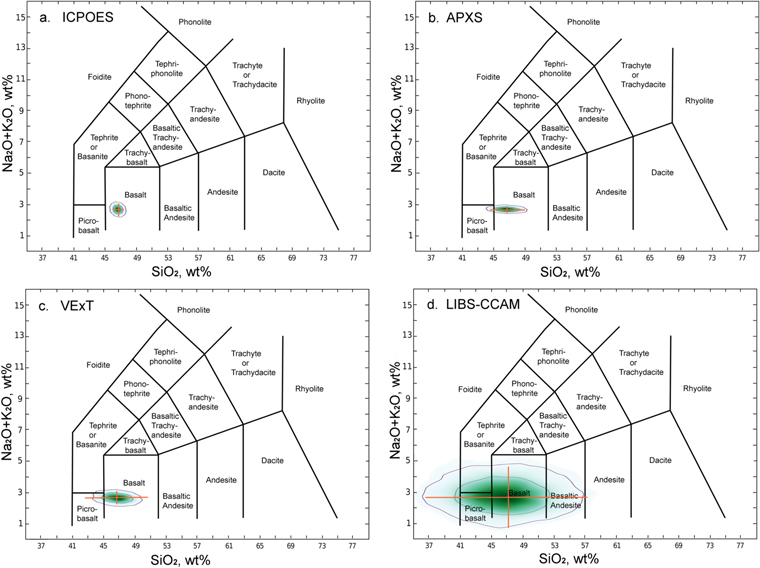
Figure 1. Total-alkalisilica (TAS) classification diagram, for the Humphrey basalt in Gusev Crater (Table 1) with applied uncertainties for each analytical method (Table 2). For each frame, 5000 points were calculated with applied uncertainties; green color intensity shows point densities; contour lines enclose 67% and 95% of points respectively (see the text). The orange bars show 2σ uncertainties calculated implicitly (see the text); note the close correspondence between the orange bars and the 95% contours. (a). ICPOES, as done in Earth laboratories (Ciborowski et al. 2015). (b). APXS, as done by MER and MSL rovers on Mars. (c). As suggested by VExT (Sharpton et al. 2014). (d). LIBS, as done by the MSL rover on Mars (Clegg et al. 2017).
Download figure:
Standard image High-resolution imageTo explore the effects of analytical uncertainties on TAS classification, we have taken as example the Humphrey basalt from Gusev Crater, Mars (McSween et al. 2006). Humphrey was among the first analytical targets of the MER Spirit rover; the chemical composition of its interior (below adhering dust and surface coating) was obtained by APXS after the surface coatings were abraded away; see Table 1 (Gellert et al. 2006; McSween et al. 2006; Filiberto et al. 2008). Humphrey contains the minerals olivine, low-Ca pyroxene, and magnetite (McSween et al. 2006; Morris et al. 2004, 2006; Ruff et al. 2006), which are consistent with its bulk composition and its classification as an olivine basalt.
In Figure 1, we compare the effects of various analytical uncertainty sets applied to the nominal bulk composition of the Humphrey basalt. The implicit calculation is shown as 2σ uncertainty bars in the directions of the graph axes; the explicit uncertainties are show as fields of varying color. The two methods coincide, except that the implicit calculation's 2σ bars are slightly smaller than the 95% contour (2σ) on the explicit; this small offset is explained above. The ICPOES uncertainties (Table 2, Figure 1(a)) represent high-quality analyses in a laboratory on Earth; its degree of uncertainty is likely near the best achievable for a natural, naturally inhomogeneous, sample (Ryder & Schuraytz 2001). The APXS and VExT uncertainties yield a larger spread of values, mostly because of their increased uncertainties in quantification of SiO2 (Figures 1(b), (c)). The LIBS uncertainties are larger than the other methods, both in SiO2 and in Na2O + K2O (Table 2, Figure 1(d)). The LIBS uncertainties yield a wide spread of possible SiO2 values, such that the Humphrey basalt might, with significant probability, be misclassified as a foidite, a picrobasalt, a basanite, or a basaltic andesite.
3.2. Chemical Index of Alteration (CIA)
The sandstones and mudstones of the Murray Formation, Gale Crater, Mars (Grotzinger et al. 2015; Fraeman et al. 2016; Stack et al. 2019), have the chemical compositions of basalts, even though they contain significant proportions of water, amorphous materials, and phyllosilicates (Rampe et al. 2017; Bristow et al. 2018; Tate et al. 2019; Thompson et al. 2020). This raises the general question of how to tell if an igneous rock has been altered by aqueous fluids, as have so many on Earth. The Chemical Index of Alteration, or CIA (Figure 2), is commonly used indicator of alteration; fundamentally, it is a measure of aluminum enrichment relative to an igneous precursor, on the theory that aqueous alteration of a rock can remove its Ca, Na, and K (from feldspars and Ca pyroxene) leaving behind the relatively immobile Al (Nesbitt & Young 1984; Nesbitt & Wilson 1992; Johnson et al. 2013). The Chemical Index of Alteration is calculated as above, Equation (2). A related presentation is the molar Al-Ca*NaK-FM ternary (Figure 3), where FM is FeO+MgO and represents abundances of mafic minerals (olivine & low-Ca pyroxene). The CIA has been applied extensively to rock chemical analyses from the Mars rovers, e.g., (McLennan et al. 2014; Cino et al. 2017; Siebach et al. 2017; Mangold et al. 2019), though it is not entirely clear if CIA is appropriate for Mars' conditions of weathering and alteration (Siebach & McLennan 2018).

Figure 2. Histograms of Chemical Index of Alteration (CIA) values for the composition of the Marimba 2 sample of the Murray Mudstone, Gale Crater (Table 1), with applied uncertainties for each analytical method (Table 2). For each frame, 5000 points were calculated with applied uncertainties; histogram of point CIA values in gray, and normal distribution curve for each in red. For the normal distribution curves (explicit calculation), 2σ values are: ICPOES, 4.6; APXS, 3.9; VExT, 7.5; and LIBS, 26. The orange bars show 2σ for each technique, calculated implicitly.
Download figure:
Standard image High-resolution image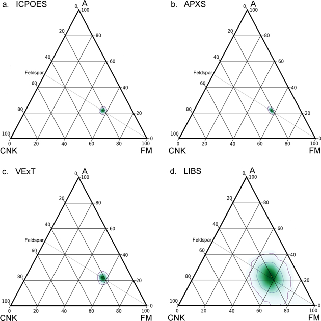
Figure 3. A-CNK-FM diagrams for the composition of the Marimba 2 sample of the Murray Mudstone, Gale Crater (Table 1), with applied uncertainties for each analytical method (Table 2). The apices of the triangles are: A, molar Al; CNK, molar Na+K+Ca; and FM, molar Fe+Mg. In each frame, 5000 points were calculated with applied uncertainties; color intensity shows point densities; contour lines enclose 67% and 95% of points respectively (see text). Analytical methods as in Figure 1 and text. Unaltered basaltic rocks tend to lie on and below the Feldspar-FM line, which is CIA = 50. Igneous rocks that plot on that line contain plagioclase, alkali feldspar, orthopyroxene, and/or olivine; most igneous rocks contain augite, so they plot below the line. Alteration of feldspar to phyllosilicates moves compositions toward the A apex.
Download figure:
Standard image High-resolution imageTo explore the effects of analytical uncertainties on CIA, we use the Marimba 2 mudstone sample from the Murray Formation, Gale Crater, for which we have both APXS and LIBS chemical analyses (see Table 1 and samples). The mineralogy of Marimba 2 is consistent with significant aqueous alteration, i.e., ∼30% (by weight) clay minerals (Mg-rich di- and tri-octahedral smectites), ∼40% amorphous material, 6.5% hematite, and ∼7% calcium sulfate (Bristow et al. 2018). Marimba 2's bulk composition (Table 1) yields CIA of ∼49, which is suggestive of aqueous alteration (Siebach & McLennan 2018); correction for the proportion of Ca sulfate in the sample raises the CIA to ∼51 (Figure 2), which is perhaps strongly suggestive of aqueous alteration.
The effects of analytical uncertainties on these measures of aqueous alteration are shown in Figures 2 and 3. Applying the uncertainties of ICPOES and APXS yield almost identical results, with a 2σ variation of ∼4 points in CIA value (Figures 2(a)(b) and 3(a)(b)). The VExT uncertainties yield more spread, approximately double that of ICPOES (Figures 2(c) and 3(c)). And the LIBS uncertainties (Table 2) yield a much larger spread, so much that one could not infer conclusively that Marimba 2 had experienced aqueous alteration (Figures 2(d) and 3(d)).
3.3. Tectonic Setting
Earth basalts are generated in a range of tectonic settings: mid-ocean ridges, continental rifts, ocean islands, subduction zones (continent–continent and continent–ocean), large igneous provinces (continental and oceanic) and so forth. For interpretation of Earth's ancient paleogeography and tectonics, it is useful to determine which of these settings an ancient basalt formed in. Most of the current discriminants for tectonic setting rely on trace elements (Pearce 1996; Vermeesch 2006; Saccani 2015; Zhang et al. 2019), and so are at present of limited utility for orbital spacecraft measurements and rover chemical analyses. A few tectonic discriminant schemes do rely on chemical analyses for major and minor elements, and we take here as an example that of Verma et al. (2006).
Verma et al. (2006) collected bulk chemical analyses of 2732 basalts (Pliocene to recent in age) from a range of tectonic settings on the Earth. Ferric iron abundances were calculated using the code SINCLAS (Verma et al. 2002). To eliminate the problem of data set closure (Chayes 1960), they used ratios of element abundances, e.g., ln(TiO2/SiO2), rather than element abundances, and applied discriminant analysis (Chayes & Velde 1965) to connect the analyses with tectonic settings. Verma et al. (2006) calculated discriminant functions, DF, for the tectonic settings island arc basalts (IAB), Columbia River Basalts (CRB, a continental large igneous province), mid-ocean ridge basalts (MORB), and ocean island basalts (OIB), and subsets thereof. Here, we use their most successful set of DF, "IAB-CRB-MORB," by which 97% of the basalts were correctly grouped to tectonic setting. The two discriminant functions here (Verma et al. 2006) are
- DF1 = −1.5736·ln(TiO2/SiO2) + 6.1498·ln(Al2O3/SiO2) + 1.5544·ln(Fe2O3/SiO2) + 3.4134·ln(FeO/SiO2)–0.0087·ln(MnO/SiO2) + 1.2480·ln(MgO/SiO2)–2.1103·ln(CaO/SiO2)–0.7576·ln(Na2O/SiO2) + 1.1431·ln(K2O/SiO2) + 0.3524.·ln(P2O5/SiO2) + 16.8712, and
- DF2 = + 3.9844·ln(TiO2/SiO2) + 0.2200·ln(Al2O3/SiO2) + 1.1516·ln(Fe2O3/SiO2)–2.2036·ln(FeO/SiO2)–1.6228·ln(MnO/SiO2) + 1.4291·ln(MgO/SiO2)–1.2524·ln(CaO/SiO2) + 0.3581·ln(Na2O/SiO2)–0.6414·ln(K2O/SiO2) + 0.2646·ln(P2O5/SiO2) + 5.0506.
The general applicability of Verma's discriminant functions is not clear (Sheth 2008) and, considering that no planet besides Earth has Earth-style plate tectonics, they may not be appropriate for Mars or Venus. We use them here as an example of the kind of interpretations that could be derived from chemical analyses of only major and minor elements.
The effects of analytical uncertainties on the Verma DF values are shown in Figure 4 for the Humphrey basalt composition (Table 1). All iron was assumed to be as FeO and the results change little for Fe3+/Fetot up to 0.25; for comparison, Mössbauer analyses suggest Fe3+/Fetot to be 0.17 (Morris et al. 2006), but this includes secondary oxidation and the original igneous oxidation state was likely lower. First, one should note that the Humphrey basalt does NOT fall into any of the Verma classification groups—its DF1 (Figure 4) is twice what any of Verma's classified compositions have. We have not done a sensitivity analysis to determine the source of this difference, but we suspect the high Fe/Mg of Mars basalts compared to Earth basalts. From Figure 4, it is clear that terrestrial ICPOES analyses give far better definition in Verma's to discriminant functions than any spacecraft method; again, we have not done a sensitivity analysis determine which factors are responsible. And, as before, the LIBS uncertainties yield a large spread of discriminant function values.
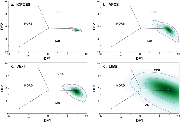
Figure 4. Verma et al. (2006) tectonic classification of the Humphrey basalt, Gusev Crater, Mars (Table 1), with applied uncertainties for each analytical method (Table 2). These diagrams show Verma's DF1 and DF2 discriminant functions among island arc basalts (IAB), Columbia River Basalts (CRB, a continental large igneous province), and mid-ocean ridge basalts (MORB). Formulae for DF1 and DF2 are in the text; these parameters for these two functions classify 97% of Earth basalts properly. For each frame, 5000 points were calculated with applied uncertainties; color intensity shows point densities; contour lines enclose 67% and 95% of points respectively (see text). Analytical methods as in Figure 1 and text. The composition of the Humphrey basalt does not fall near any of the fields for Earth basalts, all of which lie between −4 < DF1 < 4 and −4 < DF2 < 4.
Download figure:
Standard image High-resolution image3.4. Magma Genesis Conditions
The chemical composition of a basalt is controlled by the physical and chemical conditions under which it formed, and by subsequent fractionation processes. If the basalt liquid experienced little fractionation after formation, i.e., it is primitive, then its composition can be used (with additional assumptions) to retrieve the pressure and temperature at which it formed, either by silica-activity barometery and Fe-Mg-exchange thermometry (e.g., Albarede 1992; Lee et al. 2009; Lessel & Putirka 2015) or experimentally using the inverse experimental modeling approach (e.g., Asimow & Longhi 2004). The formation conditions of primitive basalts can have broad implications for the tectonic and thermal history of a planet (Dasgupta et al. 2010; Filiberto & Dasgupta 2011; Herzberg et al. 2010). These are worthy goals for a spacecraft mission, thus it is worth considering how uncertainties in chemical analyses can affect a basalt's inferred temperature and pressure of formation.
As an example, we target the Martian basalt Humphrey, analyzed by APXS by the MER rover Spirit in Gusev Crater, Mars, Table 1 (Filiberto & Dasgupta 2015; McSween et al. 2006). Humphrey is an Adirondack-class basalt, and is inferred have experienced ∼10% olivine fractionation since its generation (Filiberto & Dasgupta 2015). Filiberto & Dasgupta (2015) inferred the mantle pressure and temperature at which the Humphrey magma was generated, using the olivine–melt Mg-exchange thermometry temperature calibration A of Putirka (2005), and the silica-activity in melt pressure calibration of Lee et al. (2009) as calculated by the spreadsheet provided as a supplement to Lee et al. (2009). These specific calculations were chosen because these reproduced the experimentally determined P–T of formation for Martian basalts (Filiberto et al. 2010, 2008; Monders et al. 2007). We follow Filiberto & Dasgupta (2011) and Filiberto & Dasgupta (2015)'s calculations, and apply the uncertainties of Table 1 to the Humphrey composition to see how they would affect inferences of mantle melting conditions. In the Lee et al. (2009) supplement spreadsheet, we set the olivine-melt  to 0.36 and the mantle Mg* to 77 (Filiberto & Dasgupta 2011), the mass increment to 0.001, and Fe3+/Fetot = 0.05. In this model, olivine is added back to the bulk composition until it is in equilibrium with the mantle composition; therefore, magmas that have fractionated olivine (but not pyroxene or other minerals) can be used to calculate average pressures and temperature of formation (Lee et al. 2009).
The effects of analytical uncertainties on the inferred pressure and temperature of Humphrey's origin are shown in Figure 5; uncertainties are as above and in Table 2. Using the ICPOES uncertainties (Figure 5(a)) permits little latitude in Humphrey's origin: 1450 ± 25 °C, and 1.6 ± 0.3 GPa 2σ, nearly identical to that calculated by Filiberto & Dasgupta (2015). Results using APXS uncertainties (Figure 5(b)) yields considerably more spread, 1450 ± 50 °C and 1.6 ± 0.7 GPa 2σ, with temperature and pressure strongly correlated. The VExT uncertainties (Figure 5(c)) yield a slightly smaller temperature range, 1450 ± 30 °C, but similar range of pressure, 1.6 ± 0.7 GPa. Applying the LIBS uncertainties (Figure 5(d)), the range of inferred pressures and temperature is so large (even to negative pressures) as to be uninformative.

Figure 5. Calculated pressure and temperature of formation for the Humphrey basalt, Table 1, from Gusev Crater, Mars; see text and Filiberto & Dasgupta (2015). For each frame, 5000 points were calculated with applied uncertainties; color intensity shows point densities; contour lines enclose 67% and 95% of points respectively (see text). Analytical methods as in Figure 1 and text.
Download figure:
Standard image High-resolution image
4. Implications
Our simulations show, unsurprisingly, that the usefulness of petrologic and geochemical interpretations depend critically on the quality of the input chemical analyses. With analyses of the highest quality, one can be reasonably certain of geochemical and petrologic parameters such as classification, CIA, pressure and temperature of basalt formation, etc. As the uncertainties (precision and accuracy) of elemental analyses increase, so also decline our certainties about constraints derived from elemental abundances, and thus petrologic and geochemical inferences from them in turn. Here, we have established a method for quantifying the effect of analytical uncertainty on geochemical and petrologic inferences. Our method can easily be taken further in pursuit of specific objectives. For example, one could compute the probability that a Humphrey basalt might be classified as a basanite (Figure 1). In another example, one could compute the probability that the Marimba 2 sample was not enriched in Al (i.e., has CIA ≤ 40) and thus that its aqueous alteration was isochemical (Figures 2 and 3).
One can reasonably ask which elements are most important for geochemical inferences, and the answer depend entirely on which geochemical parameter one wants to access, and the level of uncertainty one is willing to accept. Among the parameters modeled here, SiO2 is the most important—it is a crucial for TAS classification (Figure 1), the Verma et al. (2006) tectonic discriminators (Figure 4), and the pressure and temperature of mantle melting (Figure 5). Unfortunately, LIBS analyses for SiO2 are significantly uncertain (Table 2). LIBS has relatively large analytical uncertainties for many other elements, witness their effect on the calculation of CIA values (Figures D, E). The precision of LIBS analyses can be, and are being, improved by considering statistical consideration of thousands of analyses such as the recent approach of Edwards et al. (2017). In that work in order to overcome at least some of the analytical uncertainty and to constrain general rock types in Gale Crater, density contour plots from a scatter function algorithm were produced from thousands of laser shot analyses across all igneous (and igneous-like) targets (see Edwards et al. (2017) for descriptions of this approach); however, this provides averages of rocks over a single area and not bulk composition for any specific rock investigated. While averaging in this manner provides information about the general types of rocks in the area, averages of igneous rock compositions are not necessarily petrologically meaningful, as igneous rocks are subject to considerable variations as a result of different degrees of partial melting, fractional crystallization, assimilation, which would not be full captured by averaged compositions.
4.1. Improvements
The better spacecraft analyses can become, the closer they can approach the quality (i.e., precision and accuracy) of Earth-based analytical techniques like ICPOES. The constraints on spacecraft instrumentation (e.g., mass, power, ruggedness, temperature control, limited sample preparation) mean that many Earth-based techniques are simply impossible for spacecraft, at least in the near future. However, it seems likely that existing spacecraft instruments can be improved. Table 2 shows that APXS and LIBS both have excellent precisions for most elements—the instruments detect enough photons for close quantification of most major/minor elements. The big exceptions there are in LIBS for S, Cl, and P; those elements do not ionize well under LIBS analytical conditions.
For both APXS and LIBS, nearly all of their analytical uncertainties come from accuracy, i.e., their calibrations. For APXS, uncertainties in calibration appear to derive mostly from the fitting of the X-ray background beneath the characteristic X-ray emissions of elements, and effects of sample inhomogeneity—rocks usually contain areas of different chemical compositions (e.g., discrete mineral grains); the nature of this chemical patchiness is difficult to capture, and its effects are difficult to model (Campbell et al. 2012; Berger et al. 2020; Flannigan et al. 2020). The mapping XRF instrument PIXL, on the Mars 2020 Perseverance rover, will alleviate this concern somewhat (Allwood et al. 2015; Williford et al. 2018): its data can be processed pixel-by-pixel, with more assurance that each represents a homogeneous substance.
For LIBS, the A-CNK-FM diagram provides a good example of the contrast between precision and accuracy. Figure 3(d) here shows the range of expected compositions for the Marimba 2 sample, a Murray mudstone, after applying the combined uncertainties of precision and accuracy. However, LIBS analyses for Murray mudstone samples, as a group, occupy a significantly smaller range in A-CNK-FM space, see Figure 4(b) of Mangold et al. (2019) it is unlikely that all of Mangold's samples have identical chemical compositions, so the uncertainty from LIBS precision must be smaller than the range on their Figure. Thus, the difference between our Figures 3(d) and 4(b) of Mangold et al. (2019) must come from calibration uncertainty (Table 2)—how well LIBS analyses correspond to "real" chemical compositions.
Calibration uncertainty for LIBS appears to derive from several factors: suitability of on-board standard, sufficient range of reference standards on Earth, and variability in the conditions of the plasma from target distance and laser shot power (Clegg et al. 2017). It seems likely that most of these factors could be mitigated, and thereby decrease the calibration uncertainties of LIBS results; at least some of these mitigations have been implemented for LIBS in the Mars 2020 SuperCam instrument suite (Wiens et al. 2017).
In theory, the science goals of a spacecraft mission should drive its analytical objectives, and thus the specifications of its instruments; this task belongs to the mission designers and the geochemists/petrologists on the teams. In practice, the opposite has commonly been true because of the long lead-times in development and space-qualification of analytical instruments. We believe that a significant share of the responsibility for, and impetus for, improved spacecraft analytical instruments should fall on the geochemical and petrologic communities. The design and production of adequate analytical instruments is possible only with clear statements of the petrologic/geochemical inferences possible from specific element abundances, ratios, or derived parameters, and only with clear requirements on the qualities of the analyses (their accuracy and precision) that will allow those inferences to be realized.
This material is based on work funded in part by NASA under grant 80NSSC17K0766 to AHT and JF, issued through the Solar Systems Workings program. The Lunar and Planetary Institute (LPI) is operated by Universities Space Research Association (USRA) under a cooperative agreement with the Science Mission Directorate of NASA. We appreciate assistance from S. McLennan, and are grateful to the Python programming community for open access to the codes used here (especially those in Matplotlib), and seeds for code as modified here (https://doi.org/10.6084/m9.figshare.12867035.v1). We are grateful for two anonymous reviews. LPI Contribution #2551.