


Abstract
We have searched a 2010 archival data set from the Canada–France–Hawaii Telescope for very small (km-scale) irregular moons of Jupiter in order to constrain the size distribution of these moons down to radii of ∼400 m, discovering 52 objects that are moving with Jupiter-like on-sky rates and are nearly certainly irregular moons. The four brightest detections, and seven in total, were all then linked to known Jovian moons. Extrapolating our characterized detections (those down to magnitude mr = 25.7) to the entire retrograde circum-Jovian population, we estimate the population of radius >0.4 km moons to be 600 (within a factor of 2). At the faintest magnitudes, we find a relatively shallow luminosity function of exponential index α = 0.29 ± 0.15, corresponding to a differential diameter power law of index q ≃ 2.5.
Export citation and abstract BibTeX RIS

Original content from this work may be used under the terms of the Creative Commons Attribution 4.0 licence. Any further distribution of this work must maintain attribution to the author(s) and the title of the work, journal citation and DOI.
1. Introduction
Irregular moons were likely once Sun-orbiting minor bodies that were captured by a giant planet early on in the solar system's history. The mechanism that changed the object from a heliocentric to a planet-centric orbit is still uncertain, although multiple theories have been suggested: gas drag, pull down due to sudden mass growth, and three-body interactions (Nicholson et al. 2008). Short orbital periods, eccentric orbits, and the relatively small volume of space that irregular moons occupy results in collisions significantly altering the initial population of irregular moons into today's size distribution. Still, the current size distribution of irregular moons provides some constraint on dynamical models of irregular moon systems and their initial population.
Only nine irregular moons of Jupiter were known before 1999. Thanks to wide-field charge-coupled device (CCD) cameras, an explosion of new discoveries occurred around the turn of the millennium. Since then, the number of new discoveries has dropped off, with the only survey of note in the last 10 yr being a 2017 study that found 12 new Jovian irregular moons (Sheppard et al. 2018). Before we started our work there were 71 known Jovian irregular moons, 10 of them with direct orbits and 61 with retrograde.
Irregular moons, like other small body populations, have size distributions that appear to obey an exponential law:  , where H is the absolute magnitude of the moon, N(<H) is the number of moons that have an H magnitude of "H" or less, and α is the logarithmic slope. Since moons around a single giant planet are roughly the same distance from Earth, H can be replaced with an apparent magnitude, mr
. The size distribution of Jovians is shallow at large sizes with α ≈ 0.2 for mR
< 19 (r > 10 km)
1
and α > 0.5 for mR
> 21.5 (r < 4 km; Nicholson et al. 2008; Sheppard & Jewitt 2003). In the intermediate magnitude range the size distribution exhibits "strong flattening" (α < 0.2; Sheppard & Jewitt 2003).
, where H is the absolute magnitude of the moon, N(<H) is the number of moons that have an H magnitude of "H" or less, and α is the logarithmic slope. Since moons around a single giant planet are roughly the same distance from Earth, H can be replaced with an apparent magnitude, mr
. The size distribution of Jovians is shallow at large sizes with α ≈ 0.2 for mR
< 19 (r > 10 km)
1
and α > 0.5 for mR
> 21.5 (r < 4 km; Nicholson et al. 2008; Sheppard & Jewitt 2003). In the intermediate magnitude range the size distribution exhibits "strong flattening" (α < 0.2; Sheppard & Jewitt 2003).
In this paper we describe the data set and our method for finding Jovian moons (Section 2) and how we produced our size distribution and a subsequent analysis (Section 3).
2. Current Data Set and Reduction methods
We analyzed a ∼3 hr archival Canada–France–Hawaii Telescope (CFHT) data set from 2010 that was originally taken to recover (successfully) a known Jovian irregular moon; in addition, two new moons (Jup LI and LII) above the single exposure limit of the frames were discovered and reported (Alexandersen et al. 2012). Although it was clear that this data set could have been shifted and stacked to reveal fainter moons, substantial ranges of on-sky rates and angles would need to be searched to find unknown Jovian irregulars, so this process was not attempted at the time. In the summer of 2019 we decided to cover this large shift-and-stack parameter space for the data set, as the nominal expected depth of mr ≃ 25.5 exceeded the depth of previous searches by at least a magnitude. This made a cumulative luminosity function study down to diameters below 1 km accessible, even if tracking the objects to determine orbits was impossible.
The 2010 September 8 UT field consisted of a single one square-degree CFHT MegaPrime field of 36 CCDs, centered at an offset of 15 west and 004 north of Jupiter. The images were unbinned, with a 0186 per pixel scale. There were 60 sequential 140 s exposures (with a 40 s CCD readout time), which meant this sequence lasted 3 hr. With a Jovian on-sky motion of 192 hr−1, longer exposures were precluded. The single exposures were sufficient to recover the previously known moons down to magnitude ≃24 in the best-seeing frames, and thus with 60 exposures, we expect to be able to see moons down to about 26th magnitude at the very limit of a stacked sequence.
The order of image processing was as follows: all images were aligned to the first image of the sequence, artificial moving objects were implanted in each image (details in next paragraph), the images were flux scaled relative to reference stars in the first image, and a 25 × 25 pixel sized boxcar filter was then applied to background subtract the images (for details on these two processes, see Gladman et al. 2001). This method is quite effective at minimizing stellar confusion as the moons move in front of them over the exposure sequence.
To determine our efficiency at finding moons, a random number of 600–650 artificial moons were implanted into each CCD. The magnitude, on-sky rate and position angle (PA) 2 of the implanted moons were drawn from a uniform distribution ranging from 24–26.2, 83–127 pix hr−1, and 238°–252°, respectively. The rate and PA ranges were chosen to go slightly beyond the minimum and maximum values for all known Jovian irregulars excluding Themisto (PA = 2322). We believe our exclusion of Themisto is justifiable because it travels close to Jupiter at the time (only 13' away) and is thus not reflective of the motion of a moon in our field, which is much farther away from the planet. The combination of image quality and rates of the implanted moons means the implanted moons should be trailed. The implanting software simulates trailing by splitting the signal into ten equal pieces and implant each piece, with equal time space, in each exposure. We only implanted moons on parts of the CCDs where we knew that the fastest moon would not move off the CCD during the 3 hr sequence, as this was also how the frames would be later trimmed after shifting.
Once this processing was complete, the image set was shifted at a grid of different rates and PAs and then combined using the median value at each pixel. To remove any cosmic rays or bad pixels and to lessen the presence of stars, we rejected the five highest values along with the lowest value for each pixel while combining the images. The range of shift rates and PAs were chosen to be slightly smaller than the implanted range: 85–125 pix hr−1 and 240°–250°, respectively. Using step sizes of 2 pix hr−1 and 2° produced six different shift PAs and 21 different shift rates, with a total of 6 × 21 = 126 different recombinations. We trimmed away from the stacked images any stacked pixel which would have resulted in a moon starting on that pixel leaving the field over the 3 hr sequence. This procedure, along with the original (smaller) CCD gaps, meant we were able to search about 80% of the one degree outer boundary (and all of the retained coverage reached our full magnitude depth). There are thus 36 adjacent "mini-fields" in our search.
All rates and PAs were searched methodically by two human operators using a five rate blinking sequence, with the fastest rate of the last five rates becoming the slowest rate of the next sequence (to provide an overlap). By blinking multiple rates at a time, moons can be easily identified by their characteristic pattern of coming in and out of "focus" as the recombination rate and PA gets closer and farther from the moons' actual rate and PA. Initially, each CCD was searched by both operators. After searching three CCDs, the detection of the two operators were deemed similar enough that only one operator searched subsequent single CCDs, in order to save time.
Even if it may be possible to somewhat improve this process in various ways, we note that due to the calibrated implantation of artificial objects, the effectiveness of our search is accurately measured and the subsequent debiasing is correct. That is, perhaps it is possible to search the data set more deeply, but this search's effectiveness has been determined.
3. Results
3.1. Detection Efficiency
After all rates and PAs were searched over all CCDs, the objects we detected were compared with the implanted moons. Any implanted object that was matched (within a tight tolerance) to a detection was labeled "found." Any object found that was unable to be matched to an implanted object became a candidate moon.
The fraction of implanted objects found, as a function of magnitude, over the whole field is very close to 1 on the bright end. Despite a typical moving source's path crossing several background galaxies, stellar halos, and/or bad-pixel columns, essentially all sources brighter than 25th magnitude were easily recovered. The detection efficiency then starts to drop around mr
= 25 and falls to 0.5 by mr
= 25.7 (see Figure 1, black points and the blue curve). We fit this fraction with a hyperbolic tangent function  , where A ≃ 1 is the fraction of bright objects that are detected, μ is the magnitude where the fraction drops to A/2 ≃ 0.5, and δ is a "width" of the drop. The curve of best fit for the implanted moons (blue line in Figure 1) has the parameters A = 0.998, μ = 25.69, and δ = 0.31, which we use as our detection efficiency. For the luminosity function study we term the "characterization limit" to be where the detection efficiency drops to 0.5. Therefore, our characterization limit is mr
= μ = 25.7; if brighter than this limit we have confidence that we can accurately debias the detected sample. Performing the same fit on various subregions of our field enabled the detection of a tiny drop of about 0.1 mag in the 50% limit going from the side of the field that is furthest from Jupiter to the closest. Thus there is an uncertainty of 0.05 mag on our characterization limit.
, where A ≃ 1 is the fraction of bright objects that are detected, μ is the magnitude where the fraction drops to A/2 ≃ 0.5, and δ is a "width" of the drop. The curve of best fit for the implanted moons (blue line in Figure 1) has the parameters A = 0.998, μ = 25.69, and δ = 0.31, which we use as our detection efficiency. For the luminosity function study we term the "characterization limit" to be where the detection efficiency drops to 0.5. Therefore, our characterization limit is mr
= μ = 25.7; if brighter than this limit we have confidence that we can accurately debias the detected sample. Performing the same fit on various subregions of our field enabled the detection of a tiny drop of about 0.1 mag in the 50% limit going from the side of the field that is furthest from Jupiter to the closest. Thus there is an uncertainty of 0.05 mag on our characterization limit.

Figure 1. This project's magnitude detection efficiency and cumulative luminosity function. Black data points show the binned fraction of detected implanted objects over the whole field and the best-fit hyperbolic tangent function (blue solid curve), which we use as our detection efficiency function η(mr ). The characterization limit (blue dashed line) was chosen to be where our detection efficiency dropped to 0.5. The red line represents the cumulative number of our characterized detections. Our debiased number of detections in the field (green line) were calculated by weighting each detection by 1/η(mr ), where mr is the detected object's r-band magnitude.
Download figure:
Standard image High-resolution imageThe fraction of implanted moons that were found as a function of the rate and PA is mostly constant except for small drop offs (about 10%) at the extreme minimum and maximum implanted values. This drop off is due to the implanted ranges being slightly larger than the search ranges. Since only a small fraction of our moon candidates have rates and/or PAs outside our search ranges, any effects caused by these drop offs will be negligible.
3.2. Detections
During our search activities, 55 moon candidates were discovered. Of these candidates, three were traveling faster than the fastest rate search, which raised doubt as to whether they are Jovian moons. Examining the distribution of on-sky rates of our detections, there is a clear separation between these three fast moving objects (green histogram in Figure 2) and the rest of the detections (red histogram). 3 We compared our detections with all minor bodies in the International Astronomical Union (IAU) Minor Planet database that are within 3 deg of our field center at the time of observation and have PAs between 238° and 252° (a range that encompasses the known moons). The three fast moving detections are right on the tail of the asteroid distribution (25''–41'' hr−1), which leads us to believe these objects are in fact slow-moving asteroids and will thus not be included in our analysis of the Jovian luminosity function. The region in which our moon candidates lie, 15''–23'' hr−1, contain no known minor planet, which is one line of evidence that strongly indicates our candidates are indeed Jovian moons.

Figure 2. A histogram of the on-sky rate our characterized detections (red) compared with known minor bodies that are within 3° of the center of our field and have position angles for their velocity vectors between 238° and 252° at the start of the observing sequence (blue). The green histogram bins show the three detections that are traveling beyond the Jovian irregular rates (Table 2), which we thus believe are asteroids on the tail of the asteroid rate distribution. Known minor bodies that are not shown are trans-Neptunian objects with rates less than 5'' hr−1 and near Earth objects with rates of above 50'' hr−1.
Download figure:
Standard image High-resolution imageOf the candidates, four were beyond the characterization limit of mr = 25.7 and another one of the candidate moons was found outside our search area by chance while performing astrometry and photometry on a different object. 4 The three fast, four faint, and one extra candidates are not included in the characterized sample, which thus consists of 47 moons. A full list of the characterized and uncharacterized detections are found in Tables 1 and 2, respectively. The cumulative number of our detections as a function of magnitude is shown in Figure 1 (red line). To debias the detections, we weighted them by the detection efficiency. Each detection became 1/η detections, where η is the detection efficiency at the object's measured magnitude. Only near the characterization limit does the cumulative number of debiased detections (green line) becomes noticeably different from the unbiased detections, due to η ≃ 1, except at the sharp drop off near the limit; because we have chosen to only debias down to the 50% detection efficiency, our population estimate is little affected by the efficiency correction.
Table 1. A List of All Characterized Detections
| Our Designation | Known Designation | mr |
|---|---|---|
| j20r97a28 | Hermippe | 21.8 |
| j32r104a24 | Erinome | 22.4 |
| j31r105a28 | (S/2003 J16) | 22.8 |
| j09r89a20 | Jup LIX | 23.2 |
| j35r115a26 | ⋯ | 23.3 |
| j30r97a20 | ⋯ | 23.4 |
| j25r108a26 | Jup LII | 23.6 |
| j22r91a19 | ⋯ | 23.7 |
| j31r113a26 | (Jup LXIX) | 23.8 |
| j11r99a26 | ⋯ | 24.0 |
| j22r94a24 | ⋯ | 24.0 |
| j27r97a26 | ⋯ | 24.0 |
| j03r94a24 | ⋯ | 24.1 |
| j23r95a24 | Jup LI | 24.2 |
| j20r112a25 | ⋯ | 24.3 |
| j32r98a26 | ⋯ | 24.3 |
| j23r113a27 | ⋯ | 24.4 |
| j30r114a28 | ⋯ | 24.4 |
| j24r97a22 | ⋯ | 24.5 |
| j00r92a25 | ⋯ | 24.6 |
| j22r98a18 | ⋯ | 24.6 |
| j27r118a26 | ⋯ | 24.6 |
| j33r98a22 | ⋯ | 24.6 |
| j16r108a21 | ⋯ | 24.7 |
| j20r109a31 | ⋯ | 24.7 |
| j24r98a22 | ⋯ | 24.8 |
| j29r112a25 | ⋯ | 24.9 |
| j31r94a26 | ⋯ | 24.9 |
| j21r97a26 | ⋯ | 25.0 |
| j32r97a26 | ⋯ | 25.0 |
| j13r105a20 | ⋯ | 25.1 |
| j24r113a22 | ⋯ | 25.1 |
| j28r95a26 | ⋯ | 25.1 |
| j20r93a28 | ⋯ | 25.3 |
| j22r110a23 | ⋯ | 25.3 |
| j27r116a25 | ⋯ | 25.3 |
| j31r97a22 | ⋯ | 25.3 |
| j18r92a22 | ⋯ | 25.4 |
| j30r114a19 | ⋯ | 25.4 |
| j32r98a24 | ⋯ | 25.4 |
| j34r96a22 | ⋯ | 25.4 |
| j09r109a21 | ⋯ | 25.5 |
| j33r107a23 | ⋯ | 25.5 |
| j09r111a20 | ⋯ | 25.7 |
| j09r93a20 | ⋯ | 25.7 |
| j10r109a22 | ⋯ | 25.7 |
| j12r113a25 | ⋯ | 25.7 |
Note. We give our internal designation, the MPC designation if it is previously known, and the moon's r-band magnitude. Our designations start with a "j" (for Jupiter) followed by the CCD number the moon was found on, then an "r" (for rate), followed by the rate (in pixels hr−1) that gave the best recombination, then an "a" (for angle), and lastly the angle (in degrees) that gave the best recombination. Note: the angle we use here is not the PA but 270° minus the PA. Known designations in (...) indicate that the identification was not simply at the nominal position based on the IAU MPC ephemeris.
Download table as: ASCIITypeset image
Table 2. A List of All of Our Uncharacterized Detections with Our Internal Designation and the Moon's Magnitude
| Our Designation | mr | Reason for Being Uncharacterized |
|---|---|---|
| j10r113a22 | 24.0 | Found outside search area |
| f11r133a19 | 22.9 | Moving too fast |
| f02r131a22 | 23.3 | Moving too fast |
| f17r136a22 | 24.9 | Moving too fast |
| j12r115a26 | 25.9 | Beyond mag limit |
| j07r112a24 | 26.2 | Beyond mag limit |
| j23r114a20 | 26.4 | Beyond mag limit |
| j10r89a30 | 26.5 | Beyond mag limit |
Note. The naming convention used is same as what is described in the caption of Table 1, except the three objects that we believe are moving too fast to be moons (see Figure 2) start with an "f" instead of a "j."
Download table as: ASCIITypeset image
We provide the astrometric entries (in standard Minor Planet Center (MPC) format) in Table A1.
3.3. Serendipitous Tracking
It was obvious that most of the irregular moon detections found in this pencil-beam search would be beyond the magnitude limit of other available data (because it is only another shift-and-stack pencil-beam study that could to descend beyond 24th magnitude for these rapidly moving targets). Nevertheless, we were able to identify some additional observations beyond the night of detection. We believe that essentially every object in the 15''–23'' hr−1 rate range is a Jovian moon.
Although there are hundreds of bright (visible on single images) asteroids in this field, the only two objects with mr < 22.5 that were in the field and in this rate range turn out to be the two brightest known Jovians in the field: Hermippe and Erinome (see Table 1). We believe that if main-belt asteroids were generating any significant confusion into the rate cut, it is highly likely some of them would have been bright, given how shallow the main-belt luminosity function is at these magnitudes.
Jup LIX (magnitude ∼23.2) had a 2 yr arc from observations in 2016 and 2017 and was sufficiently close to its predicted position that identification was trivial.
In the Jovian rate range, two more objects turned out to be Jup LI and LII, which is fortunate because Alexandersen et al. (2012) discovered them in this very same data set. We used no knowledge of the prior existence of any irregular in our search; we have only later identified detections in our rate range with previously known moons. With a better photometric calibration now available, we believe the original magnitudes of JLI and JLII were first reported as ≃0.5 mag brighter than they should be.
Jup LXIX was a less trivial identification. The 2017 and 2018 discovery astrometry was confined to fewer dark runs than LIX and in fact its predicted sky position was just off this 2010 data set's coverage. However, we identified j21r113a26 as close in magnitude and sky rates while being only about 4.1' away and thus believed this was a recovery of the moon. We determined this moon should then be on archival recovery observations reported in Alexandersen et al. (2012) that were targeted to track Jup LI and LII; we located and measured it. The MPC confirmed that these observations all link together, and we have thus increased the observed arc from 1 yr to 8 yr.
The object j22r94a24 was located on Palomar 5 m observations taken on the same calendar date that overlaps with this CFHT's field's coverage; these observations start roughly two hours before the CFHT data and overlap in time.
For completeness, we mention that the high-precision orbits of Harpalyke and Eurydome placed them inside this square degree, but they occupied CCD gaps at the time of our observations and were thus not detected. Note that this gap coverage is corrected for below in our estimates of the total population. Our field contained nine known moons with roughly 20% of the area lost in the shift-and-stack process; having two non-detected moons is thus unsurprising. Lastly, there are two Jovians with temporary designations (S/2003 J 9 and S/2003 J 12) whose ephemeris, based on a few-month arc from 2003, is on the field but with an enormous error (of order thousands of arcseconds according to analysis of Jacobson et al. 2012). It is possible that these moons are actually among our detections, but we have not yet been able to establish a linkage.
To summarize, every object we detected in our Jovian irregular rate cut that could get additional observations has turned out to be a Jovian irregular, leaving little credence for the argument that the fainter detections in this rate range are not Jovians. While there remains a small possibility that one of these detections happens to be a small Centaur passing close to Jupiter, our main goal is a luminosity function analysis to estimate the size distribution and the total Jovian irregular population down to magnitude 25.7; an interloper or two will have a negligible effect on these analyses.
3.4. Slope of Debiased Luminosity Function
We performed a single exponential least-squares fit on the binned differential luminosity function of both our debiased detections, from mr = 23.75 to 25.75, and on the known retrograde moons in the MPC database, starting where the size distribution starts to ramp up, mr = 21.85, to just before it rolls over, 23.05 (the reason for using just the retrograde population is explained in Section 3.5). The resulting logarithmic slopes we get from the fit for our detections and the known retrograde moons are α = 0.29 ± 0.15 (the orange line in Figure 3) and 0.6 ± 0.3, respectively. The uncertainties were obtained by generating differential luminosity functions with random numbers for each bin drawn from a Poisson distribution with the original number in each bin being the expected number of occurrences. Single exponential least-squares fits were performed on 10,000 such luminosity functions, producing a distribution of slopes; we used the full width at half maximum of this distribution as our uncertainty bounds. The two slopes are different at a level between 1 and 2σ, providing weak evidence that the luminosity function for retrograde Jovians changes to a shallower slope at mr ∼ 23.5. This is not a surprise, as simulations (Bottke et al. 2010) produce "waves" in the luminosity function as the exponential index fluctuates around the collisional equilibrium value of α = 0.5 (Dohnanyi 1969) as one moves to fainter magnitudes/smaller sizes. These waves propagate down the luminosity function as the largest objects in the finite distribution are disrupted; the fact that α is close to 0.5 usually indicates that this portion of the size distribution has "relaxed" to near equilibrium.
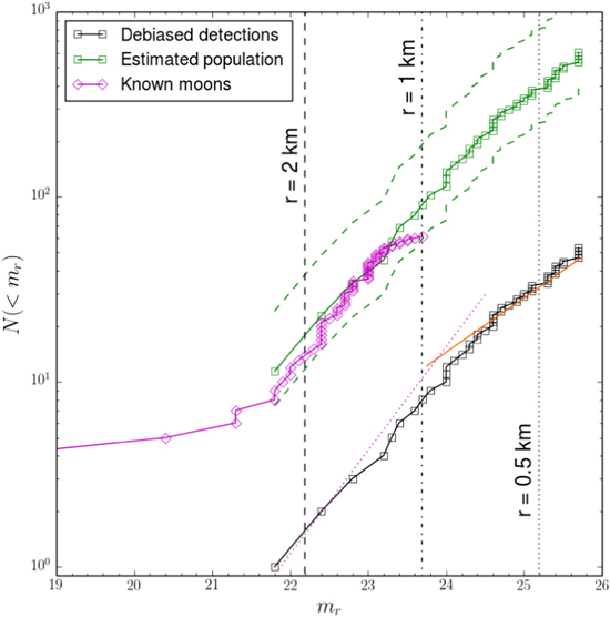
Figure 3. The black line shows the cumulative debiased number of Jovians based on our search field. The magnitude corresponding to radii of 2, 1 ,and 0.5 km (using a 0.04 albedo and Jupiter's distance at the times of the observations) are indicated by vertical lines. The solid orange line is the α = 0.29 slope of the best-fit differential luminosity function (see the text) that uses the debiased detections from mr = 23.75–25.75. We produce a total retrograde Jovian population estimate (green line) and uncertainties (green dashed lines) by applying a multiplier of 11 ± 5 (see the text) to the debiased detections; this estimate lines up nicely with the currently known population of bright retrograde Jovian irregulars (magenta line), indicating the inventory is essentially complete to mr ≃ 23.2. Our differential fit to the known retrograde moons (from mr = 21.85 to 23.05, assuming no incompleteness correction) has been shifted down to our debiased detections for reference (magenta dotted line), showing that at the bright end our detections have a similar slope but the faint end appears to be shallower. Our detected sample suggests there are ≃600 mr < 25.7 retrograde Jovian irregulars (to a factor of 2).
Download figure:
Standard image High-resolution image
3.5. Retrograde Population Estimate
We assume at this point that the vast majority of our detections have retrograde orbits. This assumption is based on (1) the edge of the field that is closest to Jupiter is about a degree away, which is approximately the projected apocenter distance of most (8 of 10) of the known direct irregular moons, and (2) only a small fraction of all known moons are direct (10/71). As such, we will make the approximation that all moons in our field are retrograde. Our analysis will thus focus on providing an estimate Jupiter's retrograde population.
We can get an estimate on the total number of Jovian irregulars if we know the fraction of the population in our field's Jovian offset at any time. We counted the average number of known retrograde moons in a field with the same size and with the same on-sky offset from Jupiter for 10 different oppositions (2009–2019). Note that over this 10 yr time interval the moons complete many orbits and thus "lose memory" of where they were discovered (most were discovered before 2004). On average there were 6.9 known moons in this field. Accounting for the 20% of sky area lost due trimming and chip gaps, on average we will detect 5.5 known retrograde moons (of 61). Thus the multiplier going from our sample to the full populations is 11 ± 5; the uncertainty value comes from the standard deviation of number of known moons over the 10 oppositions. If there were biases induced in the fraction of known retrograde moons in our field due to where the detections surveys found many orbits ago (which we think unlikely), there could be a systematic present but we believe this is likely small compared to our factor of 2 estimate.
Our estimated total population of retrograde moons overlaps nicely with the known population from mr ≈ 22–23 (see Figure 3). Beyond mr ≈ 23.2 the known population flattens out and diverges from our estimated population, indicating that the current completion limit is mr ≈ 23.2. This is in agreement with the fact that the brightest object we were unable to match to a known object has mr = 23.3.
Our results produce an estimate of 160 ± 60 retrograde Jovian moons with mr < 24, which agrees with the Sheppard & Jewitt (2003) prediction of 100 down to the same limit (although their prediction includes retrograde and direct moons). We estimate there are 600 retrograde Jovian irregulars (within a factor of 2) down to 25.7 magnitude. Using an albedo of 0.04 (the average retrograde Jovian albedo from Grav et al. 2015) and the distance of Jupiter at the time of observation produces a radius of 0.4 km for a magnitude of 25.7. We get a 10% error in the radius, which is dominated by the fact we do not know if the moon is half a Hill sphere in front or behind Jupiter. If retrograde Jovians are almost complete down to mr = 23, then the known retrograde population being well within the error bars of our population estimate suggests that we have overestimated the size our error bar; our R > 0.4 km estimate's uncertainty may thus be less than a factor of 2.
We posit that the overall completion limit for known direct Jovians would likely be at a brighter magnitude that for the retrogrades. Direct Jovian moons have smaller semimajor axes compared to retrograde moons, resulting in direct moons spending more time close to Jupiter. We speculate that this makes direct moons harder to detect and could contribute to the relative lack of direct Jovians compared to retrograde.
4. Conclusion
We found 52 Jovian moon candidates, 7 of which were previously known, from an archival data set dating back to 2010. Using artificially implant objects we were able to turn 47 of the candidates into a luminosity function of retrograde Jovian moons down to mr = 25.7. The slope we obtain from our luminosity function in the range of mr = 23.75–25.75 is α = 0.29 ± 0.15, which shows a weak signal of being shallower than the 0.6 ± 0.3 for known retrograde Jovian moons in the range of mr = 21.85–23.05. Using the mean fraction of known retrograde Jovian moons in a same sized field and the same offset from Jupiter as ours over 10 different oppositions, we scale our detections up to get an estimate on the total population of retrograde Jovians. From our analysis we get that the current completion limit of retrograde Jovian irregulars is mr ≈ 23.2 and there are (within a factor of two) 600 of these moon down to mr = 25.7.
This work was supported by funding from the National Sciences and Engineering Research Council of Canada. This research used the facilities of the Canadian Astronomy Data Centre operated by the National Research Council of Canada with the support of the Canadian Space Agency.
Appendix
Table A1 provides our MPC format astrometry and photometry. Most faint objects have just two astrometric measurements that were obtained by stacking all and then the last half of the images. We were able to get more measurements of brighter objects, which can be seen on small subset of stacked images or even single images. Some astrometric measurements do not have photometry associated with them, either due to inability to do photometry or because we thought there were already enough reliable photometric measurements for that object.
Table A1. The Format of the File Containing the Astrometry of Both Our Characterized and Uncharacterized Detections, Consistent with MPC Astrometry Submission
| Column | Use |
|---|---|
| 1 | Blank |
| 2–12 | Designation of object |
| 14 | Blank |
| 15 | "C" for CCD |
| 16–32 | Date of middle of exposure |
| 33–44 | Observed R.A. (J2000.0) |
| 45–56 | Observed Decl. (J2000.0) |
| 57–65 | Blank |
| 66–71 | Observed magnitude and band |
| 72–77 | Blank |
| 78–80 | Observatory code |
Note. This file is also available by request from the authors.
Only a portion of this table is shown here to demonstrate its form and content. A machine-readable version of the full table is available.
Download table as: DataTypeset image
Footnotes
- 1
Approximate sizes are calculated using a 4% albedo.
- 2
Here position angle is the direction of motion of an object measured counterclockwise from direct north.
- 3
The double peak in the rate distribution of the detected objects is centered on the Jovian rate and is believed to be due to the majority of the known retrograde moons having projected orbits that extend beyond our field. As such, very few come to rest relative to Jupiter in our field. Thus almost all of our detections should be going faster or slower than Jupiter's rate than at it.
- 4
This extra detection (j10r113a22) had moved into a chip gap during the observation sequence and thus was outside of our characterized search area, but it was bright enough to be seen on a subset of the images.