


Abstract
We analyze the environmental features and growth history of high-redshift halos from cosmological simulation data to determine the conditions that lead to Population III star formation. We use support-vector classification (SVC) to determine the separation in feature-space between Population III halos and halos that form no stars. We perform hyperparameter tuning but are unable to produce an SVC model that reliably classifies Population III halos. We perform feature selection and determine that among our included features, Lyman–Werner radiation and halo mass have the most significant impact on an SVC model's effectiveness.
Export citation and abstract BibTeX RIS
The lack of observational constraints on metal-free (Population III) stars has resulted in a wide range of plausible formation environments and relevant physical processes that control the formation of these first generations of stars. Models and simulations suggest that they would have formed in dark matter halos of ∼106 M⊙ and been very massive (Bromm & Larson 2004; Hirano et al. 2014, 2015) primarily due to the inefficient cooling of H2 (O'Shea & Norman 2008).
Using cosmological simulation data (Wise et al. 2012), we analyze the properties of Population III star-forming halos and compare them to halos that form no stars. We calculate halo positions and virial radii with the Rockstar halo finder code (Behroozi et al. 2012a), and construct the associated halo merger trees using the Consistent Trees code (Behroozi et al. 2012b). We define a halo to be a sphere of its virial radius, including all of its gas, stars, and dark matter. We define halo progenitors as the most massive progenitor from the previous data output taken from the merger tree. Our analysis includes 29 data outputs across a redshift range of 12 > z > 7.
Previous work (Bromm & Larson 2004; Greif 2015) has established that halo mass is the primary determinant of Population III star formation. In our simulation, no halos below several times 105 M⊙ form stars, whereas above ∼3−4 × 10⁷ M⊙, all halos form stars, regardless of any other feedback effects. Between these thresholds, some percentage of halos form stars. It is known that various physical processes and environmental effects such as H2 fraction and density, mass growth via mergers and accretion, and Lyman–Werner radiation affect Population III star formation (Bromm & Larson 2004; O'Shea & Norman 2008; Greif 2015; Griffen et al. 2017), however their relative importance has not been quantified when all of these effects are coupled. We thus restrict our analysis to this intermediate mass range. Across all data sets, we find 2003 halos in this mass range with only 62 unique halos that form Population III stars.
We are primarily interested in the characteristics of a halo's growth history and environment that influence Population III star formation. We calculate and consider the following features, where we approximate the mass derivatives with first-order accurate methods: (1) halo mass M, (2) specific mass growth rate (1/M)(dM/dt), (3) mass-normalized derivative of growth rate (1/M)(d2M/dt2), (4) redshift z, (5) number of mergers since last data output, (6) volume-averaged Lyman–Werner radiation intensity, and (7) distance to 5th nearest neighbor, a proxy for environment.
Because Population III stars affect their local environment, we compare the no-star halos to Population III progenitor halos. We find no statistically significant difference between the distributions of these two classes in any individual or pair of features. We fit the populations to a multivariate Gaussian and calculate the Mahalanobis distances for each halo. This is a generalization of the standard deviation and is a measure of how far from the mean a halo is in feature-space (Mahalanobis 1936). We found no statistically significant difference in the Mahalanobis distances between the two populations which suggests that Population III halos are not outliers in this feature-space.
To perform a more sophisticated analysis, we use support-vector classification (SVC) utilizing modules from scikit-learn (Pedregosa et al. 2011). SVC is a supervised learning method that produces a hyperplane of separation in feature-space between instances of different classes. SVC models are especially useful for classification problems in higher dimensions where visualization is not possible.
To avoid overfitting to the data, we validate the model produced by the SVC by splitting our data into a training set and a testing set. We randomly assign halos to either the testing set or the training set. The number of halos that we assign to each set is set by the variable test_size, the fraction of the whole set that goes into the testing set. We generate the model using the training set, and we then compare its classification predictions on the testing data to the true classifications.
To determine a model's effectiveness, we calculate the precision P, recall R, and F1 score, where we define P = tp/(tp + fp) and R = tp/(tp + fn). Here tp is the number of true positives, fp is the number of false positives, and fn is the number of false negatives. We consider Population III progenitor halos to be the positive class and no-star halos to be the negative class. The F1 score is the harmonic mean of the precision and recall which gives more weight to the lower of the two scores. It is a useful metric when we want to achieve high scores for both precision and recall.
We vary the hyperparameters of the SVC and test_size to determine which model yields the highest F1 score. We find that only the kernel, the penalty parameter C, and test_size affected the overall results. We use the polynomial kernel and vary test_size and C. We show the results of these variations in Figure 1. We use the defaults for all other hyperparameters. We achieve the best scores with test_size = 0.7 and C = 0.01. The highest score we achieve on the testing set is F1 = 0.24, therefore none of our models are particularly successful. The scores for the training data tend to be much higher than for the testing data, suggesting severe overfitting to the training set.
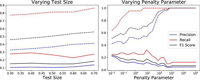
Figure 1. Precision, recall, and F1 scores of the SVC model when varying test_size and the penalty parameter C. Left panel: Variations as a function of test size while fixing C = 0.01. Right panel: Variations as a function of C while fixing test_size = 0.7. The dashed and solid lines show the scores for the training set and testing set, respectively.
Download figure:
Standard image High-resolution image
To identify the most important features for Population III star formation, we perform feature selection by removing each feature individually and calculating the decrease in the F1 score. Lyman–Werner radiation and halo mass have the greatest impact on F1 score. Removing these variables individually results in a relative reduction in F1 score of 48% and 34% respectively. Removing any other feature results in a relative reduction of 8% or less.
Overall, our methods are not successful in distinguishing Population III halo progenitors from halos hosting no star formation. Further analysis is required to reach any reliable conclusions about how the growth history and environment of a halo influence the formation of Population III stars. A larger data set that includes more samples of Population III halos could produce a more robust SVC model. Defining halos in a more sophisticated manner, including different features, and performing feature engineering may also result in better predictions.
J.G. and B.W.O. acknowledge support from NSF grants PHY-1430152, AST-1514700, AST-1517908, and OAC-1835213 and by NASA grants NNX12AC98G and NNX15AP39G. J.H.W. acknowledges support from NSF grants AST-1614333 and OAC-1835213 and NASA grants NNX17AG23G and 80NSSC20K0520. Computations and analysis described in this work were performed using the publicly available Enzo and yt codes, which are the product of a collaborative effort of many independent scientists from numerous institutions around the world. Their commitment to open science has helped make this work possible. Analysis was performed in part using the Michigan State University High Performance Computing Center (operated by the Institute for Cyber-Enabled Research).