Current Sheet Alignment in Oblique Black Hole Magnetospheres: A Black Hole Pulsar?

A black hole (BH) with a magnetic field penetrating its event horizon can be born from magnetized progenitors such as a spinning down, rotationally supported hypermassive neutron star (NS; Falcke & Rezzolla 2014) or a BH–NS merger remnant (East et al. 2021).

According to the no-hair theorem (Misner et al. 1973), the magnetic flux on a BH event horizon in vacuum will inevitably decay over time (Price 1972). However, BHs born from magnetized progenitors will, very likely, not be isolated in a vacuum but be surrounded by a (conductive) plasma, thereby changing the magnetospheric dynamics. In a stationary axisymmetric magnetosphere, poloidal magnetic field loops with their ends penetrating the event horizon can only exist if supported by non-force-free currents (MacDonald & Thorne 1982; Gralla & Jacobson 2014). It follows that in a force-free magnetosphere, an inherited closed magnetic field geometry, e.g., typically assumed to be a dipole, will inevitably evolve into a split monopole geometry (Komissarov 2004; Lyutikov & McKinney 2011; Bransgrove et al. 2021) in which the current sheet extends all the way to the event horizon. In the limit of infinite conductivity, the magnetic field would be prevented from decaying. However, in nature, although typically extremely high, a finite conductivity allows for magnetic reconnection leading to magnetic field decay (Lyutikov & McKinney 2011; Bransgrove et al. 2021). This is in contrast to the case of an NS, where reconnection occurs past the light cylinder and the flux through the assumed perfectly conducting NS surface remains unchanged (Goldreich & Julian 1969; Bogovalov 1999; Philippov et al. 2019).

A strikingly similar situation of a BH shedding its event horizon magnetic flux through magnetic reconnection could occur in accreting BHs in the magnetically arrested disk state and may result in observable powerful X-ray and gamma-ray flares (Ripperda et al. 2020, 2022; Chashkina et al. 2021; Hakobyan et al. 2023).

In previous studies, BH magnetic and rotational axes were aligned, both in 2D (Lyutikov & McKinney 2011) and in 3D (Bransgrove et al. 2021). These studies showed the formation of a split monopole geometry after an initial transient phase starting from a dipolar field. Therefore, in this work, we assume that a split monopole geometry has already formed on the event horizon. Unlike what was assumed in earlier works, it is likely that the inherited magnetosphere is misaligned with the BH spin axis. In order to study this more general scenario, we here consider a nonaccreting spinning BH magnetosphere with an initially inclined split monopole geometry in 3D.

We adopt a general relativistic (ideal) magnetohydrodynamic (GRMHD) description of the magnetospheric plasma and employ a (fixed) Kerr spacetime geometry with a range of dimensionless BH spin parameters a ∈ {0.5, 0.8, 0.9, 0.99}, BH mass M, gravitational constant G, speed of light c, and gravitational radius r_g = GM/c². The simulations are performed using the BlackHoleAccretionCode (Porth et al. 2017; Olivares et al. 2019). The GRMHD equations are solved in spherical, event-horizon-penetrating logarithmic Kerr–Schild coordinates (t, s, θ, ϕ; McKinney & Gammie 2004; Porth et al. 2017) with $s={\rm{ln}}(r)$, where t is time; r, θ, and ϕ are the spatial spherical (Kerr–Schild) coordinates; and the BH spin axis is aligned with the z-axis (i.e., along θ = 0). The Eulerian magnetic field components Bⁱ (with i ∈ r, θ, ϕ) are initialized by a split monopole magnetic vector potential ${A}_{\phi }=\left(1-\sqrt{{{\rm{\cos }}}^{2}\theta }\right)/(r\,{\rm{\sin }}\theta )$ rotated by an initial inclination angle χ₀ = 30° about the y-axis.

We impose an equation of state for a fully relativistic ideal gas with an adiabatic index $\hat{\gamma }=4/3$ initializing pressure as p(r) = Θρ(r)c² with a dimensionless temperature Θ = 0.05 for a cold plasma and ρ as the plasma density. In order to closely represent a split monopole magnetosphere with B ∼ r⁻² and ρ(r) ∼ r⁻², the initial plasma magnetization is set to σ(r) = σ₀ r⁻² = B²/(ρ(r)h) for r ≤ 2r_g (i.e., inside a radius of the maximum extent of the ergoregion) with σ₀ = 50 and where $h=(1+(\hat{\gamma }/(\hat{\gamma }-1)){\rm{\Theta }}){c}^{2}$ is the relativistic specific enthalpy. To keep the plasma magnetization from becoming so small for large radii that it would no longer represent a force-free magnetosphere, we set the initial plasma magnetization for r ≥ 2r_g to be uniform and equal to its value at r = 2r_g to σ = B²/(ρ h) = 12.5. This plasma magnetization sets the initial plasma density field ρ(r) and the initial plasma beta (i.e., gas-to-magnetic pressure ratio) β(r) = 2Θ/(1.2σ(r)) (i.e., β(r ≥ 2r_g) = 6.7 · 10⁻³).

The computational domain covers 1.01 ≤ r/r_g ≤ 400, 0 ≤ θ ≤ π, and 0 ≤ ϕ < 2π, and we run all simulations until t = 400 r_g/c. We apply the second-order accurate "Koren" reconstruction scheme as well as second-order time integration (Porth et al. 2017). To ensure the highest resolution on the inclined current sheet, we use a wedge-shaped static mesh refinement (SMR), whereby we enforce the highest refinement level within ±45° around the equatorial plane (see Figure 7 in Appendix A). We use a base resolution with 128, 64, and 128 cells along the r, θ, and ϕ coordinates, respectively, and increase the resolution by consecutively doubling the number of cells in each coordinate direction inside the SMR wedge.

To investigate numerical convergence (see Appendix A), we performed 16 simulations (labeled SMR-SP) for the four different BH spins (indicated in the simulation label by the number after "SP") using four different increasingly larger effective resolutions (indicated in the simulation label by the number after "SMR"). In addition, we performed one simulation with five refinement levels (SMR5-SP99) with a = 0.99, i.e., an effective resolution of 2048 × 1024 × 2048 cells (in r × θ × ϕ). Finally, we performed two simulations (labeled SMR4-SP99-X0 and SMR4-SP99-X20) with a = 0.99 for χ₀ = 0° and χ₀ = 20°, respectively, to investigate the dependence on the initial inclination angle.

For numerical stability, we apply a floor model where we enforce a maximum plasma magnetization with identical radial dependence as in initialization, except with σ₀ = 100 instead of σ₀ = 50. In addition, the Lorentz factor is capped at a maximum of 50 to diminish the influence of unphysical cells that can sporadically appear throughout the evolution. These can be caused by the lack of numerical accuracy when conserving momentum in the case of a too-low density leading to unphysically large Lorentz factors (see also the discussion of how this is handled in contemporary codes in Section 4.1 of Porth et al. 2019).

In this section, we describe the evolution of the initially inclined split monopole current sheet. Figures 1 and 2 show a time sequence for selected quantities at t = (45, 111, 270) r_g/c (all taken in the same phase of rotation) corresponding to the initial, intermediate, and late evolutionary phase of the highest-resolution simulation, SMR5-SP99. Figure 1 displays 2D slices of the xz-plane (side-on view of the meridional plane), and Figure 2 shows the xy-plane (top-down view of the equatorial plane).

Zoom In Zoom Out Reset image size

Zoom In Zoom Out Reset image size

Due to spacetime rotation (Lense–Thrirring frame dragging), the magnetic field lines start to corotate (i.e., rotation in the same direction as the spin of the BH), twist, and bend, extracting energy from the BH spin from the ergosphere (white dashed lines) via the Blandford–Znajek (BZ) mechanism (Blandford & Znajek 1977). Contrary to the magnetic field lines being frozen into an NS surface, the magnetic field lines penetrating an event horizon are able to slide over it. The rotational velocity Ω_F of the magnetic field, and therefore the current sheet, at the (outer) event horizon (black circles with outer event horizon radius ${r}_{{\rm{H}}}=(1+\sqrt{1-{a}^{2}}){r}_{{\rm{g}}}\approx 1.14{r}_{{\rm{g}}}$ for a = 0.99) in our simulations is Ω_F ≃ Ω_H/2, with Ω_H = ac/(2r_H) the BH angular velocity. This is in agreement with the prediction from the BZ solution (Komissarov 2004; Okamoto 2006).

The corotation of the inclined current sheet leads to an outward-moving wavelike spiral structure (i.e., an Archimedean or Parker spiral) similar to the striped wind known from oblique pulsars (Michel 1971; Kirk et al. 2009). In Figures 1 and 2, the striped wind current sheet is shown by the regions of high β (in the second row) and low comoving plasma magnetization ${\sigma }_{{\rm{co}}}={b}^{2}/(\rho {c}^{2}(1+(\hat{\gamma }/(\hat{\gamma }-1)){\rm{\Theta }}))$ (in the first row), where b is the comoving magnetic field strength. The striped wind structure occurs within an angular sector centered around the rotational equator on global scales comparable to the BH size (i.e., ∼r_g). The plasma magnetization, except in the current sheet, is σ_co ≳ 10 such that for this magnetized wind, the magnetic stresses accelerate plasma to a bulk Lorentz factor ${\rm{\Gamma }}\sim \sqrt{{\sigma }_{{\rm{co}}}}$ (see fourth row in Figures 1 and 2). In addition, the dissipation of magnetic energy into plasma energy through reconnection (effectively changing the adiabatic index) creates a radial outward pressure gradient that may enhance the radial bulk acceleration. On scales that are comparable to the current sheet thickness (i.e., smaller scales than the global scales of the striped wind), the current sheet is not smoothly shaped but locally corrugated (see Figure 1). Inside the current sheet, we find local magnetic X-lines (i.e., X-points) through which reconnection occurs, leading to the formation of flux tubes (i.e., plasmoids; Bhattacharjee et al. 2009; Loureiro et al. 2012). The plasma magnetization in regions upstream from the current sheet makes the plasma nearly force-free and results in an Alfvén speed ${v}_{{\rm{A}}}=\sqrt{{\sigma }_{{\rm{co}}}/({\sigma }_{{\rm{co}}}+1)}c\gtrsim 0.95c$ such that reconnection occurs in the relativistic regime. Consequently, the plasma inside the current sheet heats up locally to Θ ≳ 10 ∼ σ_co and becomes hotter than the surrounding plasma (see the third row in Figures 1 and 2). Inside the current sheet, magnetic tension accelerates plasma in the direction of the reconnection outflows.

As the system evolves, we observe that the corotating current sheet on the event horizon starts to tilt toward the BH equatorial plane until it has completely aligned. In other words, the current sheet inclination angle χ(t) (between the normal to the current sheet plane and the BH spin axis) decreases over time to zero (see by comparing the second, fourth, and sixth columns of Figure 1). We note that we observe this current sheet alignment in all our simulations varying in BH spin and numerical resolution. Additional simulations (Selvi et al. 2024, in preparation) show that the aligned dipole geometry will transition rapidly within ∼50 r_g/c to the split monopole geometry, which is fast compared to the alignment timescale.

As a result of alignment, the striped wind is sourced at the event horizon by an increasingly smaller opening angle over time, as shown in Figures 1. Due to the outward motion of the striped wind, this time dependence of the opening angle at the event horizon translates into a radial dependence of the opening angle leading to an amplitude-dampened striped wind. This reduction of the opening angle is illustrated by the envelope (white dashed–dotted lines in the second row of Figure 1) created by the event horizon current sheet if it would radially propagate at the speed of light. Comparing the striped wind to this envelope shows that it moves near-ballistically away from the BH with approximately the speed of light for all radii (see the first and third columns of Figures 1 and 2). So not only does the envelope have a curved shape (in contrast to the force-free case of a pulsar, where it is delimited by two diverging straight lines; Philippov & Kramer 2022), inevitably, this envelope over time will not be fixed in space but near-ballistically move outward.

The plasma motion is such that for r ≳ 5r_g, it moves approximately radially (see the 3-velocity streamlines in the fourth row of Figures 1 and 2). Furthermore, a stagnation surface located at a few r_g from the BH spin axis separates inward-moving plasma from outward-moving plasma (see the last row of Figures 1 and 2). This region, which is being vacated from matter, represents the starved magnetospheric region (i.e., gap; Levinson & Cerutti 2018; Chen & Yuan 2020; Crinquand et al. 2020; Niv et al. 2023) in which pair formation may provide the outflow of matter. Moreover, magnetized plasma can only move inward inside the inner light surface with radius $(1/4){g}_{\phi \phi }{{\rm{\Omega }}}_{{\rm{H}}}^{2}+{g}_{t\phi }{{\rm{\Omega }}}_{{\rm{H}}}+{g}_{{tt}}$ (white dotted lines), where g_{μ ν} is the metric components (Gralla & Jacobson 2014). In addition, in the outward-moving plasma, Poynting flux is converted into plasma kinetic energy through the Lorentz force acting on the matter, thereby increasing the (bulk) Lorentz factor of the plasma for larger radii (see fourth row of Figures 1 and 2).

In order to quantify the alignment, we integrate the magnetic moment density μ of the current sheet over a spherical shell of a single cell thickness Δr localized on the event horizon while neglecting radial gradients and assuming γⁱⁱ ≈ 1/γ_ii , giving $\mu =\int \int {\int }_{{r}_{{\rm{H}}}}^{{r}_{{\rm{H}}}+{\rm{\Delta }}r}r(\sqrt{{\gamma }^{\phi \phi }}{\partial }_{\phi }{B}_{r}+\sqrt{{\gamma }^{\theta \theta }}{\partial }_{\theta }{B}_{r}){dV}$, where ${dV}=\sqrt{\gamma }{drd}\theta d\phi$ is the volume element, γ is the spatial metric determinant, and γⁱⁱ is the ii-component of the spatial metric. This leads to considering only the current density tangential to the event horizon (i.e., only current density components in the θ- and ϕ-directions) or, equivalently, only the radial magnetic field component. The current sheet inclination angle χ(t) is then defined as the angle between this magnetic moment vector and the BH spin axis. This integrated measure works robustly down to χ ≃ 1°. The top panel of Figure 3 shows the time evolution of χ(t) from our highest-resolution simulations for each spin (continuous lines). After the initial transient phase t ≲ 50 r_g/c for all spins, the inclination angle decreases exponentially until the current sheet fully aligns (i.e., has an inclination angle of ≤1°). For t > 50 r_g/c, we fit the measured inclination angle with an exponential function $\propto {e}^{-t/{\tau }_{\chi }}$ to obtain the alignment timescale τ_χ . The lowest considered spin, a = 0.5, has an alignment timescale τ_χ ≃ 1118 r_g/c (green lines), which is more than an order of magnitude larger than that of the highest spin, a = 0.99, making the alignment timescale evidently dependent on the BH spin, where higher spin results in faster alignment. For the highest spin, a = 0.99 (in the highest-resolution simulation, SMR5-SP99, indicated by the black thick solid line), the current sheet aligns with an exponential alignment timescale τ_χ ∼ 85 r_g/c (indicated by the black dotted line) such that after a time evolution of ≃350 r_g/c, the alignment is complete (χ < 1°).

Zoom In Zoom Out Reset image size

To investigate the spin dependence, we relate the alignment timescale to the BH angular velocity Ω_H in units of c/r_g shown in Figure 4. By fitting the measured alignment timescales as a function of Ω_H, we find that ${\tau }_{\chi }\simeq 20{{\rm{\Omega }}}_{{\rm{H}}}^{-2}$ such that the alignment timescale is inversely proportional to the square of the BH angular velocity.

Zoom In Zoom Out Reset image size

For simulation SMR4-SP99-X20 with χ₀ = 20° (see the brown solid line in Figure 3), the exponential alignment timescale is similar to the matching case with χ₀ = 30° (see by comparing the brown dashed line to the thin black line). This implies that the alignment timescale appears independent of the initial inclination angle, at least for limited changes in the initial angle.

By comparing the electromagnetic output power of our simulations to the BZ power scaling (Blandford & Znajek 1977; Tchekhovskoy et al. 2010) while considering the instantaneous event-horizon-penetrating magnetic flux (i.e., taking flux decay into account, discussed in the next section), we conclude that the current sheet inclination angle and its alignment has no significant effect on the power extraction (see Appendix B).

During an initial transient phase, we observe that the event horizon magnetic field flux redistributes over several r_g/c into a nonuniform configuration, in which the radial magnetic field component B^r peaks at the rotational poles, is lowest at the equator, and is invariant in the azimuthal direction (see the second column of the fifth row in Figure 1). The inclined current sheet sits on top of this event horizon flux configuration as a magnetic field discontinuity. While Bransgrove et al. (2021) attributed this nonuniformity to a remnant of the initial dipole geometry, we observe that it also occurs in our split monopole simulations; therefore, we conclude that it is related to the spacetime rotation. The degree of nonuniformity depends on the BH spin, where higher spin leads to a higher degree of nonuniformity and zero spin to a completely uniform case. We quantify the nonuniformity similarly to Bransgrove et al. (2021) with a nonuniformity factor of k, where k = 1 represents a uniform distribution and for k > 1, more flux is concentrated at the poles than at the equator. We find that while for our lowest spin (a = 0.5), k ∼ 1, our highest spin (a = 0.99) has k ∼ 1.2.

Magnetic reconnection causes magnetic field lines (black arrowed lines in the fifth row of Figures 1 and 2) from the upstream regions to flow toward the current sheet, thereby dissipating magnetic field energy. Due to magnetic reconnection, the magnetic flux on the event horizon decays and, therefore, so does the radial magnetic field B^r . In order to quantify the event horizon magnetic flux decay, we consider a quantity that is closely related to the magnetic flux and that we define as ${{\rm{\Phi }}}_{| {\rm{B}}| }={\int }_{0}^{2\pi }{\int }_{0}^{\pi }| {B}^{r}| \sqrt{\gamma }d\theta d\phi$. ⁸ The bottom panel of Figure 3 shows the time evolution of Φ_∣B∣(t) normalized to its initial value Φ_∣B0∣ = Φ_∣B∣(t = 0) for all simulated spins (solid lines). For all spins and initial inclination angles, Φ_∣B∣ decreases exponentially with a similar timescale τ_Φ ∼ 2 · 10² r_g/c ranging between 179r_g/c and 236r_g/c. This means that after a time of ∼460 r_g/c, approximately 10% of the initial event horizon flux is left. The decay rate is exponential even after alignment has taken place and, in fact, is independent of the current sheet inclination angle.

We note that for higher spin (and higher resolution), the flux decay seems to be slightly slower. In order to investigate the differences between these flux decay rates more thoroughly, resistive (and even higher-resolution) simulations are required.

5.1. The Origin of Current Sheet Alignment

5.2. Observational Signatures

Precursor—The birth of a BH can lead to a number of transient electromagnetic and gravitational signatures. The perturbation of the magnetosphere may cause a monster shock (Beloborodov 2023) leading to emission preceding any observational signature created during the subsequent evolution of the magnetosphere (e.g., Nathanail et al. 2017) considered in this work. In the following, we discuss the possibility of a observational signature resulting from the current sheet alignment.

Striped wind characteristics—Our case may produce observable emission similarly to a current sheet beyond the light cylinder of a pulsar. On top of the periodic rotation, the alignment of the current sheet changes the inclination angle, leading to a striped wind with a progressively smaller opening angle. Moreover, event horizon magnetic flux loss leads to weakening of the magnetic field strength in the outward-moving wind.

This dampened striped wind is characterized by three timescales: the pulsation period P(Ω_H) = 2π/(Ω_F/2) = 4π/Ω_H, the fitted alignment timescale ${\tau }_{\chi }({{\rm{\Omega }}}_{{\rm{H}}})=20{{\rm{\Omega }}}_{{\rm{H}}}^{-2}$, and the fitted decay timescale τ_Φ = 2 · 10² r_g/c (all three timescales are shown in Figure 5 by the thick colored lines referring to the left vertical axis) with Ω_H in units of c/r_g. By inspection of the timescale expressions, we can conclude that always P < τ_χ , meaning that the signal will always be periodic (before aligning). Additionally, we can conclude that the period and the alignment timescale are related such that, at a fixed BH mass, a shorter period is always accompanied by faster alignment, and vice versa.

Zoom In Zoom Out Reset image size

We find three possible characteristic regimes of the signal. For τ_Φ ≲ P ≲ τ_χ (which holds for Ω_H ≲ 0.06 and a ≲ 0.24), assuming that our results can be extrapolated to smaller spins, the signal will weaken due to magnetic flux loss before any of the other characteristics (rotation and alignment) are able to manifest themselves in the signal (shown by the shaded region in Figure 5). For P ≲ τ_Φ ≲ τ_χ (which holds for 0.06 ≲ Ω_H ≲ 0.32 and 0.24 ≲ a ≲ 0.91), the signal is periodic while weakening in strength faster than the alignment is able to significantly affect it. For P ≲ τ_χ ≲ τ_Φ (which holds for Ω_H ≳ 0.32 and a ≳ 0.91), the periodic variation in obliquity angle (at a given azimuth) has an envelope with an increasingly smaller opening angle while weakening only on longer timescales.

BH mass and spin from striped wind characteristics—The expressions for P(Ω_H) and τ_χ (Ω_H) allow us to determine expressions for the BH mass,

$$\begin{eqnarray}&&M\sim 26\displaystyle \frac{{(P[{\rm{ms}}])}^{2}}{{\tau }_{\chi }[{\rm{ms}}]}{M}_{\odot },\end{eqnarray} \tag{ 1 }$$

with P and τ_χ in milliseconds, and for the dimensionless BH spin parameter,

$$\begin{eqnarray}&&a\sim \displaystyle \frac{20\pi {\tau }_{\chi }P}{(100{P}^{2}+{\pi }^{2}{\tau }_{\chi }^{2})},\end{eqnarray} \tag{ 2 }$$

which are applicable to all regimes discussed above. If the period and alignment timescale can be measured, the spin and mass of the BH can be directly calculated using these expressions.

Timescale restrictions from BH mass and spin bounds on NS–NS mergers—Although limitations to the possible mass of an NS depend on the still-unknown equation of state of its nuclear matter, various studies have been able to put bounds on it. The mass of a remnant BH formed from an NS–NS merger is then, in principle, bounded on the lower end by a gravitationally collapsing maximum-mass nonrotating NS (Rezzolla et al. 2018) and on the higher end by the (unlikely) merger of two supramassive NSs (Falcke & Rezzolla 2014) that are each maximally spinning, such that the range of masses we consider is 2.0 ≲ M/M_⊙ ≲ 4.8. The bounds on the BH mass put limits on the (dimensional) range of the three characteristic timescales of our signal, as shown in Figure 5 by the shaded colored regions associated with the right vertical axis (in milliseconds). For example, a maximally spinning BH (Ω_H = 1/2) with the lowest possible BH mass (M = 2 M_⊙) creates a signal with the shortest possible period P ∼ 0.25 ms and fastest possible alignment rate τ_χ ∼ 0.8 ms.

More likely, though, the spin is more moderate, resulting in a longer (and slower) pulsating signal. The maximum spin (the mass-shedding limit) of a rigidly rotating NS is constrained to a < 0.81, setting a bound on the resulting BH spin (Annala et al. 2022). Since there is plenty of orbital angular momentum available, some authors have argued that the NS–NS merger remnant should be near the mass-shedding limit (Piro et al. 2017). Moreover, it has been shown that a collapsing NS will lead to a BH with spin a < 0.68 (Lo & Lin 2011; Most et al. 2020). Thus, assuming, e.g., for a typical a = 0.6 (i.e., Ω_H = 0.17) and M = 2 M_⊙, the alignment timescale is τ_χ ∼ 7 ms with a period P ∼ 0.74 ms.

Characteristic timescales from timed pulses—We can qualitatively describe the expected observational signature of the current sheet emission by using a simplified model. We assume that (among other simplifications) the direction of emission is along the plasma velocity direction due to relativistic beaming; the plasma motion is radial for r ≳ 5r_g (see the fourth row in Figures 1 and 2); the emission originates from a fixed radius, e.g., from r = 5r_g (being close to the BH as energy density drops quickly with radius); and the emission can escape the magnetosphere toward an observer. Then a (fixed) observer receives the emission in the form of timed pulses whenever the current sheet inclination angle at the emission radius matches that of the observer.

The general shape of the emitting current sheet inclination angle $\tilde{\chi }$ (i.e., the striped wind) at a fixed azimuth can be modeled by a dampening sinusoidal as $\tilde{\chi }(t)={e}^{-t^{\prime} /{\tau }_{\chi }}{\chi }_{0}{\rm{\cos }}(2\pi t^{\prime} /P)$, with $t^{\prime} =t-{t}_{0}$ as the time offset accounting for an initial transient phase for which this fitting formula is not valid. Here, the term ${e}^{-t^{\prime} /{\tau }_{\chi }}{\chi }_{0}$ is the current sheet inclination angle χ(t). In Figure 6 (for the conditions of simulation SMR5-SP99), $\tilde{\chi }(t)$ is shown by the dashed black line, the initial transient phase by the gray shaded region, and χ(t) by the black dashed–dotted line.

Zoom In Zoom Out Reset image size

In addition, Figure 6 shows the current sheet inclination angle $\chi ^{\prime}$ measured by the maximum current density along the θ-direction at r = 5r_g at a fixed azimuth tϕ₀. We attribute the variability of the measurements of $\chi ^{\prime}$ relative to the modeled signal $\tilde{\chi }$ to the local corrugated motion of the current sheet causing deviations from the global striped wind motion. Moreover, the signal model $\tilde{\chi }$ assumes that Ω_F is exactly Ω_H/2; however, the rotational velocity is actually slightly larger. The cumulative effect of this difference becomes apparent when at later times the measured signal goes slightly out of phase with the model.

At zeroth order, the separation between two consecutive odd or even pulses received by a fixed observer (shown by the dotted horizontal line) at an angle χ_obs gives the period P (e.g., from first to third red cross). However, as a result of alignment over time, the measured time between two consecutive odd or even pulses shrinks, which is ultimately related to the alignment rate. For the special case when assuming P ≪ τ_χ , it is possible to analytically determine P and τ_χ (see Appendix C).

Emission and reconnection—The emission is expected to be produced by radiation mechanisms that are similar to that of a pulsar in the current sheet beyond the light cylinder. Merging plasmoids can eject fast magnetosonic waves that may escape as coherent electromagnetic radio emission (Philippov et al. 2019) strongly dependent on the (unknown) opacity. Furthermore, reconnection-accelerated particles may lead to X-ray and gamma-ray emission (Bai & Spitkovsky 2010; Philippov & Spitkovsky 2018; Bransgrove et al. 2021). In addition, we note that for the prediction of light curves, caustic effects known from pulsars are likely to be relevant (Bai & Spitkovsky 2010).

We estimate the cooling regime of reconnection-accelerated particles by comparing the accelerating Lorentz force to the radiation back-reaction force and assuming synchrotron cooling dominance. Given the narrow range in remnant BH mass from the NS–NS merger scenario, we arrive at the following approximate relation ${B}_{{\rm{up}}}^{3/2}\unicode{x022DA}5\gamma$ for respectively the weak (<1), intermediate (∼1), or strong (>1) cooling regime. Here, B_up is the upstream magnetic field strength in units of G and γ is the pair multiplicity (i.e., the pair density in excess of Goldreich–Julian). For a realistic scenario applicable to our work, it is unlikely that B_up and γ are such that ${B}_{{\rm{up}}}^{3/2}\lesssim 5\gamma$. Therefore, we can conclude that high-energy emission is likely to be produced by particles in the strong cooling regime.

For both high-energy emission and radio emission to be observable, they have to be able to escape the magnetosphere. Two effects that should be considered for this are high-energy photons that may annihilate into electron–positron pairs and radio emission that may be absorbed by the surrounding material. For a hypermassive NS born from an isolated progenitor (i.e., without an accretion disk or debris), the environmental absorption may not be an issue. In the case of an NS–NS merger, it is highly likely that merger debris is present, obscuring any emission. However, for a long-lived (∼day) hypermassive NS formed after an NS binary merger, it can be argued that a large portion of the debris may have been accreted or left the magnetosphere before the gravitational collapse to a BH (Rowlinson et al. 2023). Moreover, it is suggested that postmerger debris mainly resides in the equatorial plane such that emission may escape at high latitudes (Fujibayashi et al. 2018; Nathanail et al. 2020; Combi & Siegel 2023). However, also for the long-lived hypermassive NS collapsing to a BH, there is a large uncertainty in the opacity due to pair production, depending both on the emitted photons and on the seed photons that may exist in the magnetosphere. We leave calculations of the emission escaping the magnetosphere for future work.

5.3. Caveats

5.4. Main Findings

S.S. would like to thank Sasha Philippov for useful discussions and feedback. B.R. would like to thank Elias Most, Yuri Levin, Ashley Bransgrove, and Andrei Beloborodov for useful discussions. This publication is part of project No. 2021.001, which is financed by the Dutch Research Council (NWO). B.R. is supported by the Natural Sciences & Engineering Research Council of Canada (NSERC). L.S. acknowledges support from the DoE Early Career Award DE-SC0023015. This work was supported by a grant from the Simons Foundation (MP-SCMPS-00001470) to L.S. and B.R. and facilitated by the Multimessenger Plasma Physics Center (MPPC). The computational resources and services used in this work were partially subsidized by NWO domain science on the Dutch national e-infrastructure with the support of the SURF Cooperative (project No. NWO-2021.001) and partially provided by facilities supported by the Scientific Computing Core at the Flatiron Institute, a division of the Simons Foundation, and by the VSC (Flemish Supercomputer Center), funded by the Research Foundation Flanders (FWO) and the Flemish Government department EWI.

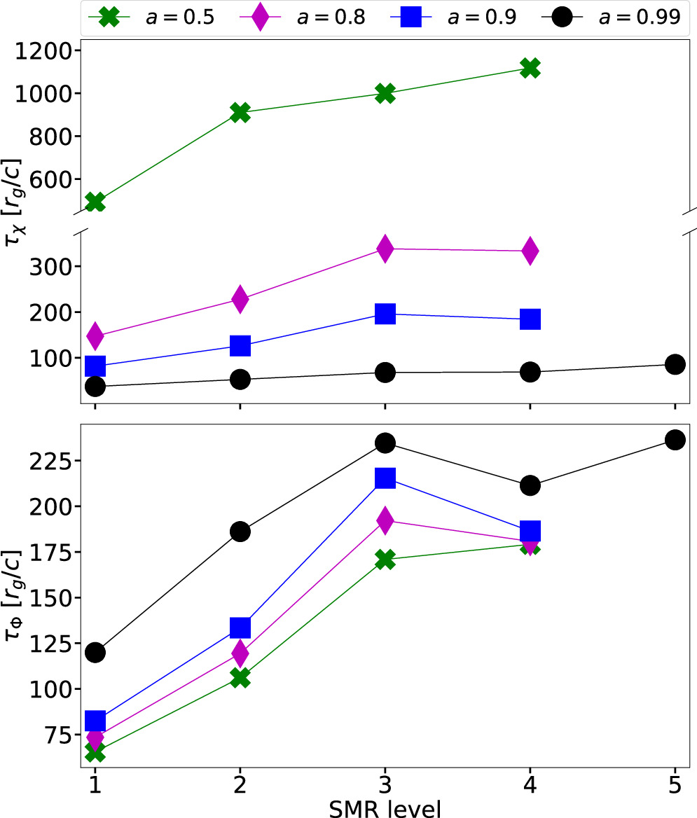
To investigate the numerical convergence of our simulations, we performed 16 simulations with an initial inclination angle of 30° for four different resolutions and four different BH spins. In addition, we performed one high effective resolution simulation for a = 0.99, which we included in our convergence study. We use SMR to refine a wedgelike structure with a half-opening angle of 45° around the equatorial region to ensure the highest resolution in the region through which the current sheet moves (see Figure 7). In our MKS coordinate system, we use a base resolution with 128, 64, and 128 computational cells along the radial, polar, and azimuthal coordinates, respectively. To increase the resolution of our simulations, we increase the level of SMR to double the number of cells in each coordinate direction inside the SMR wedge. The two quantities we focus on are the characteristic current sheet alignment timescale τ_χ of the current sheet inclination angle χ(t) and the characteristic decay timescale τ_Φ of the magnetic flux on the event horizon Φ_∣B∣ (see Section 4 for a definition of this quantity).

Zoom In Zoom Out Reset image size

Figure 8 shows the characteristic timescales τ_χ and τ_Φ in, respectively, the top and bottom panel for all spins (indicated by the connected colored markers) as a function of the resolution (indicated by the SMR level). The top panel shows that by increasing the resolution from the base level up to the third SMR level (effectively 256 cells in the polar direction) for all spins, the alignment timescale increases. From the third SMR level up to higher resolutions (i.e., effective resolution higher than 256 cells in the polar direction), we see the signs of convergence for the alignment timescale as for each spin, the relative difference between the timescales of consecutive resolutions becomes smaller (i.e., the curves for each spin flatten out for higher resolutions). Furthermore, for all simulated resolutions, the spin-dependent hierarchy of the alignment timescale is preserved such that higher spin results in faster alignment. Additionally, we note that the alignment timescale depends significantly on the BH spin such that lower spin leads to larger timescales possibly requiring higher resolutions for convergence for the lower-spin case.

Zoom In Zoom Out Reset image size

The bottom panel shows that the event horizon magnetic flux decay timescale increases up to the third SMR level. For resolutions up from the third SMR level (effectively 512 × 256 × 512 cells in the r × θ × ϕ directions), we see a nonmonotonous trend as the decay timescales of all spins of the fourth SMR level become lower (and the timescale in the single fifth-level simulation is again slightly larger). In our simulations with resolutions higher than the third SMR level, we observe that the current sheet is locally strongly corrugated and see the formation of X-points for reconnection and flux tubes (i.e., plasmoids). This may be caused by starting to resolve an instability at higher resolutions that is not resolved at lower resolutions. This may explain the behavior of the decay timescale for resolutions upward from the third SMR level. Similarly to the alignment timescale, we see the decay timescale converging as for each spin, the relative difference between the timescales of consecutive resolutions becomes smaller (i.e., the curves flatten). Furthermore, here the spin-dependent hierarchy is also preserved such that higher spin results in slower decay. By comparing the highest-resolution simulations for each spin, we can also conclude that the flux decay timescales are similar and there is no significant spin dependence for all considered BH spins. Although we can interpret the trend for the timescale upward from the third SMR level as a sign of convergence, we cannot exclude that for resolutions higher than the fifth SMR level, which is computationally unfeasible for us at this point, the trend may change again. We note that there is a discrepancy of a factor of ∼2 with the decay timescale presented by Bransgrove et al. (2021) for our initially aligned case. We have performed additional 2D simulations with an initial split monopole and dipole magnetic field geometry using resolutions comparable to our fourth SMR level, which show similar decay timescales to the 2D case of Bransgrove et al. (2021). However, our simulations in 3D with varying initial tilt angles show a decay rate that is angle-independent and in all cases a factor of 2 faster than the 3D result of Bransgrove et al. (2021; for Bransgrove et al. 2021, the 2D and 3D decay rates were equal). A more detailed investigation of this discrepancy and the differences between our approach using a 3D ideal MHD in a logarithmic Kerr–Schild coordinate grid and Bransgrove et al. (2021) using a 3D resistive MHD in an equatorially squeezed (i.e., resulting in a significantly higher resolution for an equatorial current sheet) logarithmic Kerr–Schild coordinate grid are beyond the scope of this work.

Blandford & Znajek (1977) showed that a magnetic field can extract BH spin energy in the form of outgoing energy flux according to the Power Scaling power scaling P_BZ. Several expressions for P_BZ are listed in Tchekhovskoy et al. (2010) that are valid for different ranges of BH spin and are validated by numerical simulations. The most general expression is an expansion in Ω_H up to the sixth order (Tchekhovskoy et al. 2010),

$$\begin{eqnarray}&&{P}_{{\rm{BZ6}}}{(t)=\kappa {{\rm{\Phi }}}_{| {\rm{B}}| }(t)}^{2}({{\rm{\Omega }}}_{{\rm{H}}}^{2}+\alpha {{\rm{\Omega }}}_{{\rm{H}}}^{4}+\beta {{\rm{\Omega }}}_{{\rm{H}}}^{6}),\end{eqnarray} \tag{ B1 }$$

where κ is a constant depending on the magnetic field geometry, which is 1/(6π) for our monopolar field; Φ_∣B∣(t) is our instantaneous magnetic flux; α ≈ 1.38; and β ≈ −9.2. Since ${P}_{{\rm{BZ6}}}\propto {{\rm{\Phi }}}_{| {\rm{B}}| }^{2}$, we use the instantaneous Φ_∣B∣(t) as the magnetic flux decays in our simulations.

In addition, in our simulations, we measure the output power by measuring the electromagnetic radial energy flux ${\dot{E}}_{{\rm{EM}}}$ through a spherical shell at the event horizon (e.g., Porth et al. 2019),

$$\begin{eqnarray}&&{\dot{E}}_{{\rm{EM}}}=-{\int }_{\phi =0}^{\phi =2\pi }{\int }_{\theta =0}^{\theta =\pi }({T}_{{\rm{EM}}}{)}_{t}^{r}\sqrt{-g}d\theta d\phi .\end{eqnarray} \tag{ B2 }$$

Here, $({T}_{{\rm{EM}}}{)}_{\nu }^{\mu }$ is the μ ν-component of the electromagnetic part of the energy-momentum tensor, and g is the determinant of the metric. In Figure 9, we show for all four simulated spins (for the highest-resolution simulations, SMR4-SP5, SMR4-SP8, SMR4-SP9, and SMR4-SP99) the time evolution of the measured ${\dot{E}}_{{\rm{EM}}}$ and the corresponding P_BZ6. This figure shows that for all spins during the entire evolution, ${\dot{E}}_{{\rm{EM}}}$ and P_BZ6 decrease exponentially. Furthermore, we verified that the difference between electromagnetic and total radial energy flux is negligible for all spins during the entire evolution, implying a well-magnetized system. Moreover, for all spins during the entire evolution, ${\dot{E}}_{{\rm{EM}}}$ is in excellent agreement with P_BZ6. Therefore, the current sheet inclination angle has no (significant) effect on the radial electromagnetic output flux, and we conclude that the output power of the BH magnetosphere is not dependent on the alignment process.

Zoom In Zoom Out Reset image size

Here we determine the analytical solution for the special case of P ≪ τ_χ from the pulse times t_n at the intersections between the model of the general shape of the striped wind and the observer (i.e., ${\chi }_{{\rm{obs}}}=\tilde{\chi }(t)$). In this regime, the period may be approximated by bisequential pulses (i.e., between two consecutive odd or even pulse) such that P ≈ t_n − t_n+2. For a fixed period of the striped wind signal, the time between pulses not only depends on the fixed observer angle but also changes due to alignment. At times t_I = (t_n+1 − t_n )/2 and t_II = (t_m+1 − t_m )/2, the observer inclination angles relative to the current sheet inclination angles are, respectively, ${({\chi }_{{\rm{obs}}}/\chi )}_{{\rm{I}}}={\rm{\cos }}(2\pi {t}_{{\rm{I}}}/P)$ and ${({\chi }_{{\rm{obs}}}/\chi )}_{{\rm{II}}}\,={\rm{\cos }}(2\pi {t}_{{\rm{II}}}/P)$. Then this results in an alignment timescale ${\tau }_{\chi }={({t}_{{\rm{II}}}-{t}_{{\rm{II}}})/{\rm{ln}}{(({\chi }_{{\rm{obs}}}/\tilde{\chi })}_{{\rm{II}}}/({\chi }_{{\rm{obs}}}/\tilde{\chi })}_{{\rm{I}}})$. As such, a minimum of three pulses are necessary to observationally obtain P and τ_χ .