


Abstract
The Carrington flare in 1859 September is a benchmark, as the earliest reported solar flare and as an event with one of the greatest terrestrial impacts. To date, no rigorous estimate of the energy of this flare has been made on the basis of the only direct observation available, its white-light emission. Here, we exploit the historical observations to obtain a magnitude estimate and express it in terms of its GOES soft X-ray class. From Carrington's original drawings, we estimated the area of the white-light flaring region to be 116 ± 25 msh. Carrington's account allows us to estimate the flare blackbody brightness temperature as ≈8800–10,900 K, given the most plausible interpretation of the reported flare brightness. This leads to an unprecedented class estimate of ≈X80 (X46–X126), on the modern revised GOES scale (a factor 1.43 higher than the traditional one). This substantially exceeds earlier estimates but is based on an explicit interpretation of Carrington's description. We also describe an alternative but less plausible estimation of the flare brightness, as adopted previously, to obtain a class estimate of ≈X14 (X9–X19). This now-deprecated scenario gives an estimate similar to that of with those of directly observed modern great flares. Approximations with "equivalent area," based on the Hinode observations, lead to comparable magnitudes and approve our estimates, though with a larger uncertainty range. We note that our preferred estimate is higher than the currently used value of X64.4 ± 7.2 (revised) based on indirect geomagnetic measurements.
Export citation and abstract BibTeX RIS

Original content from this work may be used under the terms of the Creative Commons Attribution 4.0 licence. Any further distribution of this work must maintain attribution to the author(s) and the title of the work, journal citation and DOI.
1. Introduction
Powerful solar flares enhance many kinds of radiation, including the optical continuum, while accelerating solar particles to high energies. Among the radiation enhancements, the broadband "white-light" (WL) emissions account for a considerable fraction of total flare radiation energy and have, therefore, long attracted scientific interest (Hudson 1972; Neidig 1989; Kretzschmar 2011). Their properties and physical mechanisms have frequently been discussed in the scientific literature (Hudson 1972; Kretzschmar 2011; Kleint et al. 2016; Kuhar et al. 2016; Benz 2017; Namekata et al. 2017; Watanabe et al. 2017; Castellanos Durán & Kleint 2020, hereafterCDK20).
These analyses are particularly important because the powerful solar flares observed in WL are occasionally accompanied by major interplanetary coronal mass ejections (ICMEs) and solar energetic particles (SEPs), which can have major impacts on space weather and modern technological infrastructure (Usoskin 2023; Hudson 2021; Temmer 2021; Cliver et al. 2022).
Solar flares have been observed since Carrington (1859) and Hodgson (1859). Since the 1970s, their magnitudes have been quantitatively measured using the soft X-ray flux (SXR) of GOES satellites (White et al. 2005; Benz 2017; Cliver et al. 2022). Among these solar-flare observations, the Carrington flare has a unique status, accommodating the first visual observations (with simultaneous confirmations) of a WL flare (Carrington 1859; Hodgson 1859) and a solar–terrestrial interaction (Stewart 1861), as well as becoming a benchmark for one of the greatest space weather events on multiple aspects: the flare magnitude, ICME velocity, geomagnetic storm, and equatorward boundary of the auroral oval (Tsurutani et al. 2003; Cliver & Svalgaard 2004; Cliver & Dietrich 2013; Hayakawa et al. 2019, 2022; Hudson 2021; Cliver et al. 2022).
So far, it has been challenging to estimate the flare magnitude of this great event, mainly because it predated modern X-ray satellite measurements (Benz 2017; Cliver et al. 2022). To date, the magnitude of the Carrington flare has been indirectly estimated as a GOES magnitude of ≈X45 ± 5 (and subsequently revised to X64.4 ± 7.2 owing to the GOES rescaling), based mainly on contemporary geomagnetic measurements for synchronized solar flare effects (Boteler 2006; Cliver & Dietrich 2013; Curto et al. 2016; Cliver et al. 2022). We regard this estimation as much more uncertain than that quoted (see Section 8).
Estimates based on direct visual observations are even more inconsistent. Measurements of the WL flaring area yielded widely disagreeing values ranging from ≈23 msh 13 (7 × 1017 cm2; Tsurutani et al. 2003) to ≈100 msh (Newton 1943), based on a close-up sketch in Carrington (1859). Tsurutani et al. (2003) suggested two magnitude estimates ≈M2 (2 × 1030 erg) versus ≈X10 (1032 erg), which differ by 2 orders of magnitude, following private communications with K. Harvey and D. Neidig. Their estimates diverged so significantly partly because they had access only to the texts and Carrington's close-up sketch (Figure 1(a)) in the classic publications (Carrington 1859; Hodgson 1859).

Figure 1. Carrington's sunspot drawings on 1859 September 1, in corrected orientations: (a) Carrington's published close-up drawing (Carrington 1859); (b) Carrington's original close-up drawing (RAS MS Carrington 1, v. 2, f. 64a); and (c) Carrington's original whole-disk drawing (RAS MS Carrington 3, v. 2, f. 313a). These images are reproduced by courtesy of the Royal Astronomical Society and were presented partially processed in Figure 2 of Hayakawa et al. (2019).
Download figure:
Standard image High-resolution imageRecent archival investigations have located Carrington's original manuscripts, not only of his close-up flare sketches but also of his whole-disk drawings (Hayakawa et al. 2018, 2019; Bhattacharya et al. 2021). Moreover, recent studies have developed statistical analyses of WL flare events (Kretzschmar 2011; Namekata et al. 2017; Watanabe et al. 2017; CDK20). These developments have enabled further detailed measurements and estimations of the magnitude of the Carrington flare. Consequently, this study aims to analyze the direct visual observations of the Carrington flare in terms of the WL-emission regions and the source active region and to compare them with modern astronomical statistics to independently estimate the magnitude of the Carrington flare.
2. Source Records and Area Measurements
Over the period 1853–1861, Carrington routinely and carefully determined the heliographic coordinates of sunspots (Carrington 1863; Cliver & Keer 2012; Bhattacharya et al. 2021) by projecting an image of the solar disk onto a coated glass plate (Carrington 1859, p. 13; Carrington 1863, Plate I). Carrington's original sunspot drawings, both whole disk and enlargements of spot groups (Hayakawa et al. 2018), are preserved in the archives of the Royal Astronomical Society (see Data Availability). Carrington's full-disk drawing for 1859 September 1 (RAS MS Carrington 3, v. 2, f. 313a) is shown in Figure 1(c). Carrington's enlarged drawing of this sunspot group in his logbook (RAS MS Carrington 1, v. 2, f. 64a) shows the WL-emission region in a reddish color (Figure 1(b)). This enlargement served as the basis for the reproduction of the figure from Carrington (1859) shown in Figure 1(a).
Carrington (1859) and Hodgson (1859) independently described the flare duration to be 5 minutes. Carrington located "the first outburst" at "not 15 seconds different from 11h 18m Greenwich mean time, and 11h 23m was taken for the time of disappearance" (Carrington 1859, p. 14), whereas Hodgson located its disappearance at "11.25 A.M." (Hodgson 1859, p. 16). Carrington reported that "two patches of intensely bright and white light broke out, in the positions indicated in the appended diagram by the letters A and B" at the flare outbreak, and "[t]he last traces were at C and D" (Carrington 1859, p. 14), indicating significant southeastward migrations of the WL-emission regions.
Following these descriptions, we measured Carrington's drawings for areas of sunspots and WL-emission regions using DigiSun, a semiautomatic software application for sunspot measurements developed at the Royal Observatory of Belgium 14 (Figure 2). A calibration step based on disk detection and the date and time allows for group-area estimation and geometrical-projection correction. First, we measured the areas of the source sunspot and source sunspot groups for the Carrington flare against a whole-disk drawing (Figure 1(c)). We measured the source sunspot group location at 21°N 14°W, near disk center. We determined the projected area on the solar disk to be 4597 msd and 5630 msd (millionths of the solar disk) and the true area over the solar surface to be 2433 msh and 2971 msh (millionths of the solar hemisphere) respectively for the source sunspot and the whole group (c.f., Watari 2022). Following Appendix A, we overlaid the snapshot drawing (Figure 1(b)) to the whole-disk drawing (Figure 2(c)) and derived the area range of the WL flaring region as 116 ± 25 msh. We consider this to be a conservative minimum estimate of the flare area, as Carrington probably missed the impulsive peak of this flare (Carrington 1859, p. 14). This is because Carrington stated as follows: "I saw I was an unprepared witness of a very different affair. I thereupon noted down the time by chronometer, and seeing the outburst to be rapidly on the increase, and being somewhat flurried by surprise, I hastily ran to call someone to witness the exhibition with me, and on returning within 60 seconds, was mortified to find that it was already much changed and enfeebled" (Carrington 1859, p, 14).

Figure 2. Screenshot of the DigiSun analysis of Carrington's WL flare emission regions (projected images). Here, we have isolated the areas of the initial flaring regions A and B (two white patches on the left), as they correspond to the impulsive phase, while those in C and D appeared only on the flare decay phase (Carrington 1859). The left-side images are reproduced by courtesy of the Royal Astronomical Society (see Figure 1).
Download figure:
Standard image High-resolution image3. Estimate of Flare Brightness
To obtain estimates for the continuum energy of the Carrington flare, we must rely upon the written descriptions of the flare brightness, based on the direct visual impression of the observers. Indeed, Carrington and Hodgson did not have any means to measure absolute light intensities. Therefore, we cannot obtain an absolute brightness determination for the flare ribbons. However, the brightness of the quiet-Sun photosphere is a well-known and very stable reference. This solar astronomical magnitude, or total solar irradiance was well known in Carrington's day, and nowadays is known to vary by less than 0.5% peak-to-peak on daily timescales, and less than a small fraction of that on solar-cycle timescales (e.g., Kopp & Lean 2011). Therefore, we could simply calibrate the brightness excess in the flaring area by determining the intensity ratio between the bright ribbons and the surrounding quiet photosphere in the image projected by Carrington's telescope. From Carrington's description, we infer that the emission was too bright for such an image comparison (flare versus disk center), but we also discuss this possibility in Appendix B.
Fortunately, Carrington explicitly tells us that "the brilliancy was fully equal to that of direct sun-light" (Carrington 1859, p. 14). Thanks to this direct comparison with an instrument-independent reference brightness, we can infer that the flare was significantly brighter than the projected solar disk, as the latter was much dimmer than direct sunlight, as seen in projection outside the telescope's image field (see the details in Appendix B). We adopt this interpretation as Optimal Scenario. The inference is that Carrington glanced at nonimaged sunlight on a convenient surface, and judged the flare brightness by this standard. To follow this up, we have estimated the relative contrast ratio, based on the known parameters of Carrington's instrument, and we combined all uncertainties, dominated by the visual error and the undocumented details of the telescope, as described in detail in Appendix C.
As long as we are trusting Carrington's descriptions, we find that the flare contrast ratio relative to the quiet solar disk must have been close to 7, with a maximum uncertainty range of 5–9, 5 being a strong lower limit with minimal assumptions on the telescope light throughput.
Hodgson (1859) also described the flare brightness, but in a much more subjective way, probably because he did not use projection, and could only use the visual image through the eyepiece (equipped with a light attenuation device for eye protection; Hodgson 1854). He emphasizes the high intensity: "a very brilliant star of light, much brighter than the sun's surface," "most dazzling to the protected eye," and "the dazzling brilliancy of the bright star α Lyrae" (Hodgson 1859, pp. 15–16). We note that Hodgson only mentions a single light source ("star"), which suggests that the angular resolution of his telescope was rather poor, and the flare image was blurred enough to prevent him from resolving the two flare ribbons. Such a degraded resolution would thus spread the light from the compact flare kernels and reduce the actual contrast relative to the solar disk. Thus, overall, Hodgson's confirmation of a bright phenomenon, even if he suffered this contrast loss, supports the high contrast of the flare derived more quantitatively from Carrington's indications.
4. Estimates of Flare Temperature and Energy
Based on the flare contrast ratio obtained in Section 3, we can further estimate the flare temperature, the bolometric radiance, and total energy. In order to derive the flare temperature, as an acceptable approximation with regard to the base observational uncertainties, we assume a blackbody emission spectrum both for the quiet photosphere and for the hot flare emission, and we combine the global spectrum with the photopic response of the human eye, as explained in Appendix D. Table 1 lists the temperatures corresponding to the median and limit values of the flare contrast.
Table 1. Brightness Temperature Tflare Derived for the Minimum, Median, and Maximum Contrast Ratio Derived from Carrington's Flare Brightness Estimate (Table A1) and GOES X-Ray Class Derived for the Different Contrast Ratios and for Two Empirical Scaling Laws
| Contrast Ratio | Tflare (K) | Eflare (erg) | X-Ray Class (SR12) | X-Ray Class (SH13) |
|---|---|---|---|---|
| 5 (minimum) | 8800 | 3.60 × 1032 | 40 | 52 |
| 7 (median) | 9900 | 5.80 × 1032 | 76 | 83 |
| 9 (maximum) | 10,900 | 8.48 × 1032 | 130 | 121 |
Note. For the latter, we used the mean values of estimates from SR12 and SH13, as explained in Section 5. The resultant X-ray class estimates are further rescaled by a factor of 1.43 for all 1–8 Å SXR peak fluxes in the pre-GOES 16 satellites (Cliver et al. 2022, Section 8.2.1; Machol et al. 2022, p. 5).
Download table as: ASCIITypeset image
Based on this flare temperature, we can then derive the bolometric radiance of the flare through the brightness estimate in Section 3 and the three assumptions in Appendix D. The temperature dependence for a blackbody is given by the Stefan–Boltzmann law:

where σ denotes the Stefan–Boltzmann constant and  and
and  denote the brightness temperature and area of the WL-emission region, respectively. Then, the total bolometric energy released by the Eflare can be written as

where τ denotes the flare duration. Based on our analysis in Section 2, Carrington's records indicated the area of the flaring region to be 116 ± 25 msh ≈3.52 ± 0.75 × 10¹⁴ m2 and the flare duration to be ≈300 ± 60 s (5 minutes).
Therefore, adopting from Table 1, a brightness temperature of 9900 (+1000, −1100) K, we thus find for the bolometric power

and for the total energy

The main contribution to the final uncertainty is the temperature raised to the fourth power in Equation (1), making the result very sensitive to the flare brightness estimate. As we actually provide the maximum range of observational uncertainties rather than an rms error, the uncertainty range of the final result must also be understood as a conservative full range rather than an rms standard deviation, hence the quite large values.
5. Conversion from Flare Energy to a GOES X-Ray Class
Figure 22 of Cliver et al. (2022) shows three empirical scaling laws between this bolometric energy and the GOES X-ray class, of which two relations mark the outer limits: a slightly nonlinear law (Schrijver et al. 2012, hereafter SR12) and a simple fully linear law (Shibata et al. 2013, hereafter SH13). These crude relations differ by up to a factor of 4, but all three laws almost coincide over the X10 to X100 range, limiting the discrepancies. Moreover, we need to rescale all 1–8 Å SXR peak fluxes in the pre-GOES 16 satellites by a factor of 1.43 (Cliver et al. 2022, Section 8.2.1; Machol et al. 2022, p. 5). This scale correction affects all the existing scaling laws using the GOES X-ray class before 2022. Therefore, we can adopt a median value between the two scaling laws by taking the arithmetic mean of converted values listed in Table 1, which corresponds to an X80 class, with a possible full range from X46 to X126.
6. Alternate Brightness Interpretation
We considered another possible interpretation of Carrington's statement "fully equal to the direct sun-light," assuming that Carrington only paid attention to the projected image, and "direct sun-light" would mean the light from the quiet solar disk. In this interpretation, the word "equal" would thus mean that the flare adds an extra brightness equal to the disk background, i.e., the flare ribbons are simply twice as bright as the background photosphere. Then, applying exactly the same procedure as in the previous section, with a contrast ratio of only 2 and also with a ±25% uncertainty, we find a brightness temperature of 6800 ± 400 K, a bolometric radiance Lflare = 4.27 ± 0.94 × 10²² W, and a bolometric energy Eflare = 1.28 ± 0.38 × 1032 erg. Using the median between the two scaling laws used in the previous section, this value can be converted to ≈X14 in the mean value within the uncertainty range X9–X19, incorporating the correction factor of Section 8.2.1 of Cliver et al. (2022). However, as discussed in Appendix D, human vision does not allow us to estimate the exact difference between two objects of different brightness. Therefore, it is dubious if Carrington could have told with any certainty that the brightness was doubled without a third external brightness reference. Moreover, the weak brightening assumed here is not consistent with Hodgson's statement for the "dazzling brilliancy" of this flare, nor with Carrington's own description involving direct (i.e., nonimaged) sunlight.
Interestingly, Hodgson (1859) also compared this flare with α Lyrae (Vega). Although he never alludes to colors and only describes how the "brilliant star" looked like on the Sun (rays and halos probably produced by optical imperfections in his telescope), we can still speculate about Vega's relatively blue color associated with its stellar class of A0. This corresponds to a high effective temperature T ≈ 10,000 K (Kowalski et al. 2017). This temperature is thus reasonably consistent with the brightness temperature derived from Carrington's flare contrast (Table 1). Moreover, the slight bluish hue of hot stars like Vega only weakly varies with temperature, and Vega was not observable during daytime anyway. Therefore, this good match is most probably attributed to a lucky and unintended coincidence.
7. Energy Estimate from an Empirical Scaling Law Based on the WL Flare Area
We also estimate the GOES X-ray flux of the Carrington flare more indirectly, based on an empirical relationship between the GOES X-ray flux and WL-emission "equivalent area" as reported by Wang (2009). The equivalent area, analogous to the equivalent width of a spectral line, is the contrast-weighted area of the flare emission as a fraction of the solar disk. Section 2 indicates an area for the WL-emission region (Aflare) to be 116 ± 25 msh, and hence an equivalent area of 218 ± 46 msd ≈631 ± 133 arcsec2.
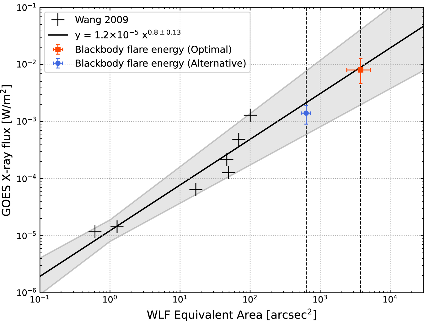
We take them to represent the equivalent area, and thus we contextualize Carrington's flare based on Wang's empirical statistics (Wang 2009), who analyzed the area of WL-emission regions using high spatial and temporal resolution observations of the Hinode/Solar Optical Telescope (SOT; see Table 1 of Wang 2009). Here, we used Wang's Hinode/SOT data (Wang 2009) for his six largest events, rescaled them with Machol et al.'s announcement (2022), and derived the empirical relationship, as shown in Figure 3:


Figure 3. Comparisons of the WLF equivalent area in arcsec2 (EAflare× (contrast – 1), following Wang (2009), and GOES SXR flux in W m−2, following Table 1 of Wang (2009), on the basis of Hinode/SOT WLF observations. The red and blue error bars include those for flare areas and resultant magnitude estimates from our photometric discussions. The gray shades indicate error margins for those for flare areas and resultant magnitude estimates from this figure's fitting parameters. The advantage of this purely empirical method is that in this estimation we do not make any assumptions about flare temperature and spectral shape.
Download figure:
Standard image High-resolution imageThis power-law relationship allowed us to estimate the GOES X-ray flux of the Carrington flare as ≥X89 (X14–X545) for the Optimal Scenario and ≥X21 (X5–X87) for the Alternative Scenario on the same basis as used before. As shown in Figure 9 of CDK20, Kretzschmar (2011) and CDK20 also described the relationship between flare energy and the WL-emission area. However, these data sets have some disadvantages for discussions of Carrington's WL-flare (WLF) sketch. CDK20 seemingly detected more WL-emission regions using the Solar Dynamics Observatory/Heliospheric and Magnetic Imager continuum (by 1 order of magnitude) than did other studies, because they detected even small WL emissions using their original automated detection methods (Figure 9 of CDK20). Their detection capability was considerably better than Carrington's detection ability, which was based on a visual inspection of a solar image on a projection screen. Therefore, their scaling underestimates the GOES X-ray class of the Carrington event. FollowingCDK20's empirical correlation (Figure 9 of CDK20), this value allows us to estimate the X-ray flux of the Carrington flare to be ≈X4.9. Kretzschmar's (2011) WLF data were not obtained from spatially resolved data but from Sun-as-a-star data. Consequently, we did not use these data for comparison with the Carrington event in this study.
8. Summary and Discussions
This Letter analyzed direct visual observations of the Carrington flare, based on Carrington's report and original drawings for the source active region, the WL-emission region, and the whole-disk solar surface on 1859 September 1. Using multiple methods, we obtained estimates as given in Table 2. These estimates reflect the limited means and precision available to the original visual observers. Our result indicates the flare magnitudes of ≈X80 (X46–X126) and ≥X89 (X14–X545) in the GOES X-ray scale, while an alternate interpretation leads to less extreme values of ≈X14 (X9–X19) and ≥X21 (X6–X87).
Table 2. Summary of Our Estimates for Brightness Temperature (Temp) and Magnitude of the Carrington Flare (Flare Mag)
| Photometric Estimate | Empirical Scaling | |||
|---|---|---|---|---|
| Optimal Scenario | Alternative Scenario | Optimal Scenario | Alternative Scenario | |
| Temp (K) | 8800–10,900 K | 6800 K | 8800–10,900 K | 6800 K |
| Flare Mag | X80 | X14 | X89 | X21 |
| Lower Estimate | X46 | X9 | X14 | X5 |
| Upper Estimate | X126 | X19 | X545 | X87 |
Download table as: ASCIITypeset image
Our visual magnitude estimates have large uncertainties, but indicate a significantly upward revision of the magnitude estimate for the Carrington flare in the Optimal Scenario (more likely) and a more conservative revision in the Alternative Scenario (less likely), when compared with independent estimates for this flare's GOES class on the basis of their correlation with solar flare effects (SFEs; geomagnetic "crochets"): >X10 (Cliver & Svalgaard 2004), ≈X15–X42 (Clarke et al. 2010), ≈X45 ± 5 (Cliver & Dietrich 2013), and ≈X45.7 ± 2.2 (Curto et al. 2016), all in terms of the original GOES scaling. These indirect estimates are based on modern-era geomagnetic crochets (SFEs) coincident with the flare in the Kew magnetogram (Stewart 1861; Bartels 1937). For consistency with the current GOES scale, the latter need to be further rescaled by a factor of 1.43, then giving X64.4 ± 7.2 (Cliver et al. 2022, Section 8.2.1; Machol et al. 2022, p. 5).
Moreover, while the nominal SFE-based estimates seem reasonable, the published uncertainty ranges can only be lower limits, because of the known systematic factors. Caveats must be noted here, as there are some variable quantifications in the SFE magnitudes for the Kew magnetogram during the Carrington SFE (Clarke et al. 2010; Curto et al. 2016) and the direction of the Carrington SFE was misinterpreted from negative to positive in some cases (e.g., Figure 5 of Curto et al. 2016; see Figure 1 of Bartels 1937). The SFE magnitude at Kew is also under debate (Clarke et al. 2010; Curto et al. 2016). The geomagnetic records for the Carrington event itself have been well preserved and publicized under the British Geological Survey (Beggan et al. 2023), which could allow us to revise the estimate in the future. The largest solar flares saturated the measurements in the GOES X-ray satellites but also are deficient in number relative to the power-law occurrence distribution function (e.g., Nita et al. 2002). Their revisions will modify the existing empirical models for the flare–SFE relationship and potentially improve the SFE-based estimate for the Carrington flare even upward. Therefore, the visual estimates remain fundamentally important. Future systematic research on SFE behavior may improve the uncertainties by better characterization of modern data in terms of its systematic parameter dependences.
We draw two main conclusions here: first, most probably, the Carrington flare was at least comparable to or even larger in total energy than the most energetic events of the better-documented recent era, such as SOL2003-11-03, and second, the radiated energy of a solar flare can indeed significantly exceed 1032 erg (or even possibly closer to 1033 erg), in accordance with results from Emslie et al. (2012) for three events with directly observed bolometric energies >3 × 1032 erg. Our results allow us to contextualize the Carrington event based on statistics of solar flare observations (Hudson 2011; Benz 2017), bridge observations and statistics of solar flares and stellar superflares (Namekata et al. 2017, 2022; Notsu et al. 2019; Okamoto et al. 2021; Cliver et al. 2022), discussions and modeling efforts on the greatest space weather events, and their impacts on modern civilizations (Riley et al. 2018; Hudson 2021; Hapgood et al. 2021; Cliver et al. 2022).
Acknowledgments
We thank the Royal Astronomical Society for letting us access and analyze Richard Carrington's original sunspot drawings and the Royal Observatory of Belgium for letting us use their measurement software application DigiSun. This work was financially supported in part by JSPS Grant-in-Aids JP20K22367, JP20K20918, JP20H05643, JP20K04032, JP21H01131, JP21J00106, and JP21K13957, JSPS Overseas Challenge Program for Young Researchers, and the ISEE director's leadership fund for FY2021, Young Leader Cultivation (YLC) program of Nagoya University, Tokai Pathways to Global Excellence (Nagoya University) of the Strategic Professional Development Program for Young Researchers (MEXT), and the young researcher units for the advancement of new and undeveloped fields, Institute for Advanced Research, Nagoya University of the Program for Promoting the Enhancement of Research Universities. Y.N. was also supported by NASA ADAP award program No. 80NSSC21K0632 (PI: Adam Kowalski). F.C. and S.B. acknowledge financial support by the Belgian Solar-Terrestrial Center of Excellence (STCE). Hi.Ha. thanks Kanya Kusano for his helpful advice. Hi.Ha. and Hu.Hu. appreciate the hospitality of Physics and Astronomy Group of the University of Glasgow. Hi.Ha. acknowledges the International Space Science Institute and the supported International Teams #510 (SEESUP, Solar Extreme Events: Setting Up a Paradigm), #475 (Modeling Space Weather And Total Solar Irradiance Over The Past Century), and #417 (Recalibration of the sunspot Number Series). Hi.Ha. also acknowledges the ISWAT-COSPAR S1-01 and S1-02 teams. We thank Olivier Boulvin for taking photograph of the projected solar image and direct Sun light at the USET telescope in Royal Observatory of Belgium.
Data Availability
Carrington's manuscripts that we used in this article are preserved in the Royal Astronomical Society in the following shelf marks. RAS MS Carrington 1 hosts three volumes of Carrington's logbooks for sunspot observations in 1853–1861. RAS MS Carrington 3 hosts three volumes of Carrington's whole-disk sunspot drawing in 1853–1861 and 1870.
Appendix A: DigiSun and Measurement of White-light Flaring Regions
The DigiSun software estimates the image-plane area of the WL flare in millionths of a solar disk (msd), based on the number of pixels above an intensity threshold, separating the pencil gray color from the whole-disk area. In addition, it calculates the true area on the solar spherical surface in millionths of a solar hemisphere (msh) by taking into account the foreshortening of each pixel based on its angular distance from the center of the Sun.
In order to measure the area of the flare ribbons, which are not depicted on the whole-disk drawing, we then overlaid Carrington's close-up drawing (Figure 1(b)) on his whole-disk drawing (Figure 1(c)), as shown in Figure 2, in order to bring it to the exact scale of the whole solar disk. However, Carrington's close-up drawing and whole-disk drawing do not perfectly match one another, mainly because smaller individual sunspots do not fall exactly on the same location. Therefore, we estimated areas for the range of scales of the close-up drawing that provided a valid match of the details in the sunspot group. The lowest and highest values of possible scaling are 90% and 100%, thus a ±5% scale uncertainty; the corresponding measured areas are given in Table A1.
Table A1. Projected Areas on the Solar Disk (PA), in Millionths of a Solar Disk, and True Areas at the Solar Surface (TA), in Millionths of a Solar Hemisphere for the Two White-light Flare Ribbons (A and B, Respectively), as Measured with the DigiSun Software for Three Different Scale Factors Applied to the Close-up Drawings to Match the Reference Full-disk Drawing
| Close-up Drawing Scale | A | B | ||
|---|---|---|---|---|
| PA (msd) | TA (msh) | PA (msd) | TA (msh) | |
| 90% | 95.4 | 50.8 | 101 | 53.4 |
| 95% | 107.3 | 57.1 | 110.7 | 58.6 |
| 100% | 128.8 | 68.6 | 135.5 | 71.7 |
Download table as: ASCIITypeset image
For the best-fitting scale of 95%, regions A and B span 107.3 msd and 110.7 msd, respectively, and 218.0 msd in total, for the projected areas, and 57.1 msh and 58.6 msh, respectively, and 115.7 msh in total for the true areas (Table A1). The ±5% scale uncertainty gives a ±10% uncertainty on the true area. Imprecisions in the marked outline of the flare ribbons raise this graphical uncertainty a bit to 15%, as shown in Table A1. Taking into account the angular resolution of a 4.5 inch aperture (1.1 arcsec), the uncertainty on the angular and true area due to the limited optical sharpness of the focal image amounts to 15%. Combining with the above 15% graphical uncertainty, this gives a 21% overall uncertainty on the area. Therefore, the A, B and A + B projected areas are 107.3 ± 23 msd, 110.7 ± 23 msd, and 218.0 ± 46 msd, while the A, B and A + B true areas are 57.1 ± 12 msh, 58.6 ± 12.5 msh, and 115.7 ± 24.5 msh.
Appendix B: Interpretation of Carrington's Brightness Description
Carrington's description of his visual observation is expressed as follows: "My first impression was that by some chance a ray of light had penetrated a hole in the screen attached to the object-glass, by which the general image is thrown into shade, for the brilliancy was fully equal to that of direct sun-light; but, by at once interrupting the current observation and causing the image to move by turning the R.A. handle, I saw that I was the unprepared witness of a very different affair" (Carrington 1859, pp. 13–14).
Carrington was thus surprised to see a bright spot that he did not believe first to be possibly part of the projected solar image (certainly because it was much too bright compared to anything he had seen during his countless hours spent observing sunspots; see Carrington 1863). Probably, the only idea that comes to his mind is that such a bright spot must be artificial, and accidentally caused by a ray of direct sunlight leaking through a hole in the occulting disk that is permanently mounted near the (front) objective end of his refracting telescope (Figure 2 of Cliver & Keer 2012). This occulter casts a shadow on the projection screen to entirely shade the screen on which the solar image is projected by the telescope. We note that this was a real possibility as the aperture of Carrington's telescope was 4.5 inches (Cliver & Keer 2012, p. 5), and thus the diameter of the telescope tube was hardly wider (probably ≈5 inches), while the projected solar image had a much larger diameter of 11 inches (Carrington 1859, p. 13), and the circular occulting screen was even wider. Therefore, any hole within a ring with a inner diameter of 5 inches and an outer diameter of 11 inches would inevitably fall somewhere inside the projected image of the solar disk, although it would be highly unlikely to coincide with the sunspot group as sketched.
The projected image is dimmer than ambient solar light (see the picture in Figure B1 and the quantitative determination below). The only bright comparison that Carrington could have found inside the dome must have been a surface exposed to direct sunlight (possibly a sheet of the paper used for solar drawings, which he had at hand). Therefore, he could have noticed the similarity in brightness, hence his initial interpretation as a light leak. Even more importantly, Carrington states that the brightness of the flare ribbons was fully equal to direct sun-light, which is a more quantitative estimate, indicating that he went beyond a vague qualitative impression (see Hodgson1859) and made a thoughtful comparison. In order to remove any doubt, Carrington, who spontaneously demonstrates here his long experience in visual observing (Carrington 1863), then immediately stopped the R.A. tracking, seeing that the bright spot started to move and maintained its position relative to the sunspots on the drifting solar disk, while a light leak would have remained fixed on the projection screen. He thus obtained instantaneous proof that something very unusual was actually taking place on the Sun itself.

Figure B1. Sample picture showing the strong intensity contrast between the projected solar image and direct sunlight falling on an identical white projection sheet, as photographed at the Royal Observatory of Belgium (ROB) in Brussels on 2023 April 4 at 14:21 UT (picture courtesy of Olivier Boulvin). Here, the telescope has an aperture of 16 cm and it projects a 25 cm solar-disk image. This historical Merz–Grubb telescope from the late 19th century has been used for the sunspot drawings at the ROB since about 1885, and its optics are comparable to the instrument used by Carrington (https://www.sidc.be/uset/telescopewlvisual.php#).
Download figure:
Standard image High-resolution imageAppendix C: Determination of the Optical Flare Contrast Ratio
When projecting the solar image, the total incoming light captured by the entrance aperture of the telescope is spread over the circular disk of the projected solar image. Therefore, the intensity of the projected disk equals

where Ii is the intensity of the solar incident light, Dt is the diameter of the objective, and Dp is the diameter of the projected solar disk.
For full precision, we must take into account the limb darkening for broadband white light, following Sánchez-Bajo & Vaquero (2002):

with uλ = 0.613 in the y spectral band (green-yellow, 510–580 nm) and θ as the central angular distance.
With this expression, the intensity at the limb amounts to 40% of the central intensity Iλ (0), while the mean disk intensity amounts to 80% of this central intensity Iλ (0). Therefore, for the central part of the disk where the flare was located, we should multiply the mean intensity of the solar disk Ip, given by Equation (C1), by 1/0.8 = 1.25.
This gives a base dimming ratio, due to the geometrical-projection scale, of

As the aperture was 4.5 inches, while the projected Sun had a diameter of 11 inches (Carrington 1859; Cliver & Keer 2012), we get rd = 4.78, i.e., the direct incident light is then about 5 times brighter than the solar disk in the projected image.
However, we must also take into account the optical efficiency of the telescope optics, i.e., the fraction of incoming light transmitted through the whole optical system. At the epoch of Carrington, optical lenses were made of bare glass, without any antireflection coating. We must thus consider the fraction of light reflected at each glass–air surface, which is given by the Fresnel equation, for normal incidence:

where n0 is the refraction index of air (=1) and nG is the refraction index of glass. nG = 1.52 for ordinary crown glass (borosilicate, BK7) and nG = 1.62 for flint glass (F2). This implies a loss of R = 0.04 for crown glass, which is used for most ordinary lenses and R = 0.056 for the flint component used in the usual doublet-lens achromatic objectives of the 19th century. This reflective light loss is independent of the wavelength, and thus the telescope optics do not modify the spectral distribution of incident light. The objective itself thus contains two lenses, and an eyepiece is needed to focus the prime-focus image on the screen. The most basic eyepiece types, like the Huygens or Ramsden eyepieces, contain two lenses, but it is likely that for obtaining a good optical quality over the whole solar disk, a three-lens eyepiece was used. Therefore we must count at least 8 optical surfaces, and more probably 10, of which 1 was a flint glass element in the objective. Assuming that no significant absorption loss occurs over the glass thickness, the transmitted light simply equals 1 − R, and the overall optical transmittance of the system equals

where N is the number of air–glass surfaces. Assuming a minimum of four lenses, To = 70%, or assuming five lenses, To = 64%. (NB: as a validation, the authors verified the above calculations by applying them to the Merz–Grubb refractor used for sunspot drawings at the Royal Observatory of Belgium, a comparable historical instrument of the late 19th century. 15 ) Given this further dimming of the projected image, the above dimming factor rd , must be multiplied by 1/To, giving a contrast ratio between direct sunlight and the quiet photosphere in the projected images of 4.78/0.70 = 6.83 (four lenses) or 4.78/0.64 = 7.47 (five lenses). As Carrington states that the flare had the same brightness as direct sunlight, those two values correspond to the brightening of the flaring ribbons relative to the surrounding photosphere, as estimated visually.
In this respect, we should consider the precision of this visual intensity estimate. Indeed, while it is easy to tell visually which of two light sources is the brightest, it is almost impossible to estimate quantitatively by how much, as the eye is a fully relative light detector. However, when assessing the equality of two light sources, the precision becomes much higher, and from statistics of thousands of visual measurements of variable stars using comparison stars, this comparative rms error was found to be only 2% (Price et al. 2007). Therefore, Carrington presumably adopted the sensible approach of looking for a source with a brightness equal to the white-light flare. Still, if two light sources do not have the same area or are surrounded by backgrounds of different intensities, the comparison may be affected by a bias. The flare was a small patch surrounded by a significantly darker background (by a factor ≈7, as found above), and the patches of direct sunlight that Carrington could use as reference may have been quite different in terms of area and surrounding background. We will never know what reference he actually used, if any. Therefore, we take a very conservative estimate of a factor of 1.50 (50% uncertainty range) for his comparative brightness estimate, i.e., ±25% around the above contrast factors, thus about 10 times the base 2% error for ideal visual comparisons of stars, which give the ranges in Table C1.
Table C1. Mean Contrast Ratio, and Extreme Range for That Ratio, Assuming Four or Five Lenses in the Optical Train of Carrington's Telescope
| Lenses | Mean | Min | Max |
|---|---|---|---|
| 4 | 6.83 | 5.12 | 8.54 |
| 5 | 7.47 | 5.60 | 9.34 |
Download table as: ASCIITypeset image
Combining all uncertainties, dominated by the visual error and the undocumented details of the telescope, the visual brightening of the flare must have been between 5 and 9, with a median value of 7 (decimals are irrelevant here, given the limited precision).
Finally, in the above calculations, we neglected the diffuse ambient light falling on the projection screen. Indeed, for a proper visibility of sunspots, the contrast of dark umbrae should hardly be reduced. Therefore, as the intensity in the core of umbrae is about 10% of the intensity of the quiet photosphere, the diffuse light must not exceed a few percent. As the flare was even brighter, this diffuse light is negligible with regard to the total uncertainties (<1%).
Appendix D: Conversion of the Visual Contrast into a Blackbody Brightness Temperature
We based our calculations on the following assumptions:
- 1.Given the position of the flare, about 20° from disk center, we can neglect the effect of the limb darkening, both for the quiet photosphere as for the flaring region. The limb darkening factor varies with the cosine of the central angle and here is close to 1 (cos(20°) = 0.94). Moreover, it is the same for the flaring source and the surrounding photosphere.
- 2.As visual observations integrate the solar irradiance over the whole visible range, the spectral distribution of the quiet-Sun radiance can be approximated by a blackbody at a temperature of 5770 K (see the verification below and Figure D1).
- 3.The emission spectrum of the flaring region can also be approximated by a blackbody spectral distribution, which uniquely defines the effective temperature
 . Modern data still do not characterize white-light flare spectra very well, and in general an optically thin chromospheric contribution may be present (e.g., Fletcher et al. 2007) and this could systematically bias the estimate in an unknown manner.

In addition, linking the visual brightness estimate to a blackbody spectrum also requires knowledge of the spectral sensitivity of the detector, here the human eye. As the observations were made in bright-light conditions, we can thus use the "photopic" response of the human eye, noted Rvis(λ), which peaks at a wavelength λ of 555 nm. We used the Commisssion Internationale de l'Éclairage (CIE) international standard photopic response (CIE 2019) illustrated in Figure D1. Note that we assume that the "pale distemper of straw," mentioned by Carrington for the glass plate used for the projection, did not significantly affect the observed spectral distribution.

Figure D1. The photopic sensitivity curve for the human eye (+), with weighting for photospheric temperature (blue) and 10,000 K (red) blackbody spectra, normalized to peak, according to CIE (2019).
Download figure:
Standard image High-resolution image
The visual intensity perceived for a blackbody emission at temperature T is thus given by

where Iv is the perceived visual intensity and IT (λ) is the Planck blackbody spectral radiance for an effective temperature T:

For illustration, the blackbody spectral irradiances for two temperatures (5770 K and 10,000 K) weighted by this photopic response are shown in Figure D1, where all curves are scaled to their respective peak values. Most of the visible signal comes from the range 450–650 nm. Moreover, although a source at 10,000 K peaks at 290 nm in the near-UV, the blue excess is very small and accounts for a difference of only 1% in the blue wing of the curves. This probably explains why neither Carrington (1859) nor Hodgson (1859) mention any special color of the flaring region. The slight bluish hue was probably too subtle to be clearly noticeable. Only Hodgson (1859), when he makes a very subjective comparison with a bright hot star—"and the center might be compared to the dazzling brilliancy of the bright star α Lyrae"—may have been inspired by a slightly "cold" hue of the flare, knowing that Vega has a spectral type of A0 and effective temperature of 9600 K.
As an example, Table D1 lists the blackbody radiances at 5770 K and 10,000 K, and their ratios at 555 nm, at the extremities of the visible range and integrated over the visible range or the whole spectrum. The latter corresponds to the bolometric radiance given by the Stefan–Boltzmann law (Equation (1)). One can see that because the hot flare plasma at 10,000 K emits a significant fraction of its light in the near-UV, the increase of the radiance in the visible range is lower than the T4 dependency (by about 20%), which leads to an underestimate of the flare temperature by about 800 K, a very significant error, if the bolometric intensity is used instead of the visible-light intensity.
Table D1. Blackbody Spectral Radiance at Specific Wavelengths, over the Visible Range and over the Whole Spectrum for Two Temperatures (Photosphere and Flare Plasma at 10,000 K)
| λ (nm) | IT at T = 5770 K (107 W m−2 μm−1) | IT at T = 10,000 K (107 W m−2 μm−1) | Ratio |
|---|---|---|---|
| 450 (blue) | 7.98 | 86.4 | 10.82 |
| 555 (green) | 8.04 | 57.5 | 7.15 |
| 650 (red) | 7.11 | 39.6 | 5.57 |
| Peak | 8.23 (at 502.2 nm) | 128.7 (at 289.8 nm) | 15.64 |
| Visible (450–650 nm) | 1.58 (107 W m−2) | 12.0 (107 W m−2) | 7.59 |
| Total (bolometric) | 6.28 (107 W m−2) | 56.7 (107 W m−2) | 9.02 |
Download table as: ASCIITypeset image
Another consequence of the weak influence of the different spectral distribution between 6000 and 10,000 K is that the ratio of intensities at two temperatures computed over the whole photopic sensitivity range or at its peak at 555 nm is essentially the same. We found that the difference in the derived brightness temperatures based on those two options is less than 50 K.
Therefore, we determined the blackbody temperature for the flare producing a brightness increase at 555 nm equal to the contrast ratios determined in Section 3. The results are given in Section 4 and Table 2.
Footnotes
- 13
Here, we abbreviate millionths of the solar hemisphere as msh.
- 14
- 15