


Abstract
The population of small, close-in exoplanets is bifurcated into super-Earths and sub-Neptunes. We calculate physically motivated mass–radius relations for sub-Neptunes, with rocky cores and H/He-dominated atmospheres, accounting for their thermal evolution, irradiation, and mass loss. For planets ≲10 M⊕, we find that sub-Neptunes retain atmospheric mass fractions that scale with planet mass and show that the resulting mass–radius relations are degenerate with results for "water worlds" consisting of a 1:1 silicate-to-ice composition ratio. We further demonstrate that our derived mass–radius relation is in excellent agreement with the observed exoplanet population orbiting M dwarfs and that planet mass and radii alone are insufficient to determine the composition of some sub-Neptunes. Finally, we highlight that current exoplanet demographics show an increase in the ratio of super-Earths to sub-Neptunes with both stellar mass (and therefore luminosity) and age, which are both indicative of thermally driven atmospheric escape processes. Therefore, such processes should not be ignored when making compositional inferences in the mass–radius diagram.
Export citation and abstract BibTeX RIS

Original content from this work may be used under the terms of the Creative Commons Attribution 4.0 licence. Any further distribution of this work must maintain attribution to the author(s) and the title of the work, journal citation and DOI.
1. Introduction
The observed population of small, close-in exoplanets with radii ≲4R⊕ and orbital periods ≲100 days (e.g., Borucki et al. 2011; Howard et al. 2012; Fressin et al. 2013; Silburt et al. 2015; Mulders et al. 2018; Zink et al. 2019; Petigura et al. 2022) provides an intriguing problem in terms of their formation pathway. With no analog in our solar system, such planets have been observed to bifurcate into two separate subpopulations, centered at ∼1.3R⊕ (referred to as "super-Earths") and ∼2.4R⊕ (referred to as "sub-Neptunes"). In between, there exists an absence of planets, labeled as the "radius gap," which decreases in size with increasing orbital period (e.g., Fulton et al. 2017; Van Eylen et al. 2018; Berger et al. 2020a; Petigura et al. 2022).
Two categories of evolutionary models have emerged to explain this phenomenon. The first relies on atmospheric evolution as it is known that many sub-Neptunes require a significant H/He-dominated atmosphere to explain their observed mass and radius (e.g., Weiss & Marcy 2014; Jontof-Hutter et al. 2016; Benneke et al. 2019). Under this class of models, super-Earths are expected to have lost their primordial atmosphere and are thus observed at their core 3 radius. Sub-Neptunes, on the other hand, have maintained their atmosphere, bloating their size to the observed peak at ∼2.4R⊕. Typically, atmospheric mass loss is thought to cause this bifurcation, with smaller-mass, highly irradiated planets losing their hydrogen atmospheres to become super-Earths, while larger-mass, colder planets remain as sub-Neptunes. Two successful mass-loss models are X-ray or extreme ultraviolet (EUV) photoevaporation, which relies on high-energy stellar flux (e.g., Owen & Wu 2013; Lopez & Fortney 2013), and core-powered mass loss, which calls upon remnant thermal energy from formation and bolometric stellar luminosity (e.g., Ginzburg et al. 2018; Gupta & Schlichting 2019). Other models may also explain the radius gap via atmospheric escape due to giant impacts (e.g., Inamdar & Schlichting 2016; Wyatt et al. 2020) or through gaseous accretion of primordial atmospheres (e.g., Lee & Connors 2021; Lee et al. 2022).
An alternative model to the retention of H/He atmospheres is the "water-world" hypothesis, in which the radius gap arises due to a difference in planet composition, with super-Earths consisting of a silicate-iron mixture and sub-Neptunes consisting of an ice-silicate mixture. Since a planetary core of a given mass increases in size for lower bulk densities, the water-world/sub-Neptune population exists at a larger size and hence separated from the rocky/iron-rich super-Earths (e.g., Mordasini et al. 2009; Raymond et al. 2018; Zeng et al. 2019; Mousis et al. 2020; Turbet et al. 2020).
These two end-member evolutionary models are not, however, mutually exclusive. Planets are likely to harbor H/He-dominated atmospheres as well as water content (i.e., Venturini et al. 2016; Lambrechts et al. 2019; Mordasini 2020; Venturini et al. 2020), which may interact with each other, as well as the silicate mantle and iron core of the planet (e.g., Dorn & Lichtenberg 2021; Schlichting & Young 2022; Vazan et al. 2022). While the specifics of these interactions remain uncertain, what remains clear is that the key to determining the nature of such planets is to ensure that models are consistent with demographic observations, i.e., can reproduce a clean radius gap with the correct orbital period and stellar mass dependencies. This naturally requires a distinct difference in bulk densities between super-Earths and sub-Neptunes.
In this Letter, we focus on a specific class of hypothesized water worlds, namely that of 1:1 silicate-to-ice ratios in the absence of H/He-dominated atmospheres. Such compositions arise as a result of condensation models of solar composition gas at fixed pressure 4 (e.g., Zeng et al. 2019). Under such models, volatiles condense beyond their respective ice line and are speculated to form the constituents of growing planets, typically via pebble accretion. Once planets are sufficiently massive, they migrate inwards toward the typical orbital periods that are observed today (e.g., Lodders 2003; Bitsch et al. 2015; Brügger et al. 2020; Venturini et al. 2020).
The nature of sub-Neptunes in this latter scenario is thus in direct disagreement with alternative models that include a single formation pathway for super-Earths and sub-Neptunes in conjunction with an atmospheric escape model. For example, inferences from photoevaporation and core-powered mass-loss models require that both super-Earths and sub-Neptunes have core bulk densities roughly consistent with that of Earth (∼5.5 g cm−3 for a 1M⊕ core), suggesting that they formed through the same pathway and divided as a result of atmospheric escape (e.g., Gupta & Schlichting 2019; Wu 2019; Rogers & Owen 2021; Rogers et al. 2023).
In a recent study, Luque & Pallé (2022) asserted that there is evidence for a population of the aforementioned water worlds among planets orbiting M dwarfs by comparing observed planet masses and radii with various planet-composition models in the mass–radius diagram. They find that many planets in their sample are consistent with a 1:1 silicate-to-ice composition ratio, as well as population synthesis modeling from Burn et al. (2021). They also use the mass–radius relations for rocky bodies hosting H/He-dominated atmospheres from Zeng et al. (2019) to claim that the planet sample was inconsistent with rocky cores hosting H/He atmospheres. Unfortunately, these adopted mass–radius models for H/He-dominated atmospheres were not appropriate for planets at fixed ages, i.e., analogous to stellar isochrones. In order to do this analysis, one must consider the thermal evolution and atmospheric mass loss with the associated changes in entropy of H/He atmospheres over time.
In this Letter, we calculate physically motivated, self-consistent, population-level mass–radius relations for rocky planets hosting H/He atmospheres, which crucially take into account atmospheric evolution and irradiation from the host star. We compare these relations to the data compiled within Luque & Pallé (2022) in Section 3, with discussion and conclusions found in Section 4.
2. Method
It is commonplace for mass–radius diagrams to be used as a visual guide to the population of observed exoplanets (e.g Wu & Lithwick 2013; Hadden & Lithwick 2014; Weiss & Marcy 2014; Dressing et al. 2015; Rogers 2015; Wolfgang et al. 2016; Chen & Kipping 2017; Van Eylen et al. 2021). To interpret the observations, theoretical mass–radius relations are used to plot a planet's size as a function of mass for a given composition. For solid bodies consisting of iron, silicate, and ice-mass fractions, the models of Fortney et al. (2007) and Zeng et al. (2019) are commonly used, in which the planet radius Rp scales approximately as  , where Mp is the planet mass (Valencia et al. 2006). Specifically the models of Zeng et al. (2019), which were adopted in Luque & Pallé (2022), give the following mass–radius relation for water worlds consisting of a 1:1 silicate-to-ice ratio:
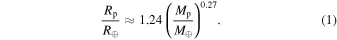
We highlight again that, for the remainder of this Letter, we define water worlds as planets with a 1:1 silicate-to-ice ratio, as in Luque & Pallé (2022), and thus follow the mass–radius relation given in Equation (1).
Our task is to determine the mass–radius relation for rocky/iron-rich cores with a H/He-dominated atmosphere. Crucially, we aim to calculate physically motivated, self-consistent mass–radius relations, which incorporate the physics of atmospheric evolution, including mass loss and cooling, which strongly modifies the mass–radius relation from the canonical H/He results of Zeng et al. (2019). We highlight that the H/He mass–radius models from Zeng et al. (2019) assume constant specific entropy in a purely adiabatic atmosphere. The assumption of constant specific entropy (which sets the adiabat) for planets of varying mass is not accurate for planets that have undergone thermodynamic processes such as cooling and mass loss, which naturally reduce the specific entropy of a planet and depend on many variables such as planet mass and equilibrium temperature. Moreover, in the Zeng et al. (2019) mass–radius relations, each model's specific entropy is parameterized with a temperature defined at a fixed pressure of 100 bars. We note that this temperature is often mistaken for the equilibrium temperature of a given planet. The temperature and density of a purely adiabatic atmosphere will drop far below the equilibrium temperature within a few scale heights of the planet's surface. In reality, an outer radiative layer will form as a planet comes into radiative equilibrium with the host star (e.g., Guillot 2010; Lee et al. 2014; Piso & Youdin 2014; Ginzburg et al. 2016). We point the reader to the mass–radius relations of Lopez & Fortney (2014) and Chen & Rogers (2016), which account for thermal evolution, including radiative-convective models that provide planet size at a constant age for a given mass and H/He mass fraction.
2.1. Constructing Mass–Radius Relations
Atmospheric mass loss sculpts the exoplanet population such that planets with larger core masses and therefore deeper gravitational potential wells retain larger atmospheric masses. This is also true for planets at cooler equilibrium temperatures since they receive a smaller integrated stellar flux, which drives hydrodynamic escape. While one can explore these basic dependencies analytically (see Appendix), the easiest way to fully understand these effects, in conjunction with thermodynamic cooling and contraction, is with numerical models. We use the semianalytic numerical models for XUV photoevaporation from Owen & Wu (2017) and Owen & Campos Estrada (2020) and core-powered mass loss from Gupta & Schlichting (2019) and Gupta et al. (2022) to numerically model populations of planets undergoing atmospheric mass loss driven by both mechanisms (see Rogers et al. 2021 for a full discussion of both models). For both models we assume an atmospheric adiabatic index of γ = 5/3, a core heat capacity of 107 erg g−1 K−1 (Valencia et al. 2010), and an opacity scaling law of κ ∝ Pα Tβ , where α = 0.68, β = 0.45, and κ = 1.29 × 10⁻² cm2 g−1 at 100 bars and 1000 K (Rogers & Seager 2010). Both models rely on the hydrodynamic escape of hydrogen-dominated material; hence we expect the predicted mass–radius distributions to be very similar.
Chronologically speaking, there are three dominant atmospheric processes that small, close-in exoplanets with H/He-dominated atmospheres undergo. First, atmospheric mass is accrued via core-nucleated accretion while immersed in a protoplanetary disk (e.g., Rafikov 2006; Lee et al. 2014; Piso & Youdin 2014; Ginzburg et al. 2016). Then, as the disk disperses, the atmospheric mass of some planets is rapidly removed through a "boil-off" process (also referred to as "spontaneous mass loss") as the confining pressure from the disk is removed on timescales ∼105 yr (e.g., Ikoma & Hori 2012; Owen & Wu 2016; Ginzburg et al. 2016). This is appropriate for smaller-mass planets ≲10M⊕ since larger-mass cores may open gaps in the gaseous protoplanetary disk, resulting in different atmospheric evolution during disk dispersal. Finally, once the disk has completely dispersed, these latter processes transition into XUV photoevaporation and core-powered mass loss (e.g., Lopez & Fortney 2013; Owen & Wu 2013; Ginzburg et al. 2018; Gupta & Schlichting 2019) combined with thermal cooling and contraction.
Since we are not explicitly incorporating gaseous accretion and boil-off, our initial conditions must encompass such processes. To account for both scenarios, namely in which boil-off does/does not occur, we adopt two sets of initial conditions. The first scenario assumes that planets have undergone a boil-off phase during disk dispersal, for which we assume that planets host an initial atmospheric mass fraction according to

which comes from the theoretical predictions of Ginzburg et al. (2016), which account for core accretion and boil-off. In the inference work from Rogers et al. (2023), the authors showed that this relation can be accurately recovered from the data by inferring the correlation between core mass and atmospheric mass fraction prior to XUV photoevaporation for a sample of Kepler, K2, and TESS planets.
In the second scenario, we do not enforce a boil-off phase. There is currently uncertainty as to the details of this mechanism, as it is a nonstandard escape process, particularly at high masses whereby gaps can be opened in the protoplanetary disk. In light of this, we provide an additional agnostic set of initial atmospheric mass fractions, drawn log-uniformly in the range

where  is a log-uniform distribution, where the lower limit avoids large mass cores hosting negligible atmospheric mass fractions (we assume planets with X ≤ 10−4 to be completely stripped, i.e., super-Earths), while the upper limit is chosen to avoid self-gravitating atmospheres, which are known to be extremely rare and which the semianalytic models do not account for (Wolfgang & Lopez 2015; Rogers et al. 2023). In essence, this distribution accounts for all possible initial atmospheric conditions. As we shall show, even this agnostic set of initial conditions accurately reproduces the observations.
We assume planetary cores are of Earth-like composition, such that they have a silicate-to-iron ratio of 67:33 (Owen & Wu 2017; Gupta & Schlichting 2019; Rogers & Owen 2021), making use of the mass–radius relations from Fortney et al. (2007). To approximately match the stellar sample from Luque & Pallé (2022), we adopt a Gaussian stellar mass distribution centered at 0.3M⊙ with a standard deviation of 0.1M⊙. We evolve a population of 105 planets for each mass-loss model for 5 Gyr to match the approximate ages of observed planets although this final age makes no difference to the final mass–radius distribution. 5 We randomly draw orbital periods from a broken power law:

where a = 1.0, b = −1.5, and P0 = 8.0 are chosen to approximately match the population of observed planets orbiting M dwarfs from Kepler (e.g., Petigura et al. 2022). We also place an upper limit on orbital periods of 30 days since most M-dwarf orbiting planets with measured masses and radii are observed with TESS, which has a baseline capable of observing planets out to this orbital separation. We randomly draw the planet core masses in a log-uniform manner so as to evenly sample the mass–radius diagram. Finally, we remove planets with an RV semiamplitude ≤30 cm s−1 to approximate current RV sensitivity limits.
3. Results and Discussion
3.1. Mass–Radius Relation for Sub-Neptunes with Rocky Cores and H/He Atmospheres
Figure 1 demonstrates the mass–radius relations for a population of rocky cores, initially hosting H/He-rich atmospheres, that have undergone thermal evolution and atmospheric mass loss over 5 Gyr. Since both photoevaporation (see left-hand panels) and core-powered mass-loss models (see right-hand panels) derive from hydrodynamic escape mechanisms, their predictions are very similar in this plane. The bimodal distribution is clearly seen, with super-Earths typically residing at orbital separations corresponding to higher equilibrium temperatures and having been stripped of their hydrogen-dominated atmospheres. As such, super-Earths fall on an Earth-like composition line in the mass–radius diagram. Sub-Neptunes, on the other hand, maintain, despite some atmospheric mass loss, a H/He atmosphere, the amount of which scales with core mass among other variables, such that more massive cores retain larger atmospheric mass fractions. These H/He atmospheres increase the radii of sub-Neptunes above that expected for an Earth-composition core. We note that the mass–radius relation for planets in the absence of atmospheric mass loss, i.e., constant atmospheric mass fraction (e.g., see Figure 1 of Lopez & Fortney 2014) is less steep than the H/He mass–radius relations from Zeng et al. (2019) (see Section 3.3). Hence, the mass–radius observations for sub-Neptunes can only be fit with H/He atmospheric mass fractions that scale with planet mass, which is a natural outcome of the hydrodynamic atmospheric-loss processes discussed above.
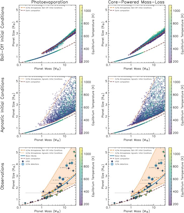
Figure 1. Synthetic mass–radius distributions are shown for populations of planets evolved with photoevaporation and core-powered mass loss in left- and right-hand panels, respectively, colored by their equilibrium temperatures. Super-Earths are stripped of their H/He-dominated atmospheres and fall onto a relation consistent with an Earth-like composition (brown dashed line), while sub-Neptunes retain a significant atmosphere. In the top panels, we assume an initial distribution of atmospheric masses appropriate for a boil-off scenario (Equation (2)), in which planets lose a significant amount of H/He mass during disk dispersal. We characterize the resulting narrow mass–radius distribution with a median line (orange dashed line; Equation (5)). In the middle panels, we adopt agnostic initial conditions (Equation (3)) and parameterize this mass–radius relation with 2σ limits (orange dotted lines). In the bottom panels, we compare our theoretical mass–radius distributions (orange dashed and dotted lines; Equation (5)) with the observed sample of M-dwarf orbiting exoplanets from Luque & Pallé (2022), together with the mass–radius relation for water worlds (blue solid line; Equation (1)). We find that boil-off initial conditions provide mass–radius relations that are completely degenerate with that of water worlds. Furthermore, even when adopting agnostic initial conditions, the observations are accurately reproduced since the mass–radius distribution is naturally explained due to mass loss and cooling/contraction of H/He-dominated atmospheres. We highlight planets with confirmed escaping H/He detections with blue-shaded regions (namely, K2 18 b, GJ 3470 b, GJ 436 b, and, tentatively, GJ 1214 b).
Download figure:
Standard image High-resolution imageIn the top and middle panels, we show mass–radius distributions for both sets of initial conditions: boil-off (see Equation (2)) and agnostic (see Equation (3)), respectively. One can see that the boil-off scenario produces a narrow mass–radius distribution, while the agnostic initial conditions produce a wider range in sub-Neptune radii for a given mass, owing to the increased range in initial atmospheric mass fractions. Note, however, that even with this set of agnostic initial conditions, the majority of sub-Neptunes sit at small radii, close to the models that started with boil-off initial conditions. This is because thermal evolution and mass loss of H/He-dominated atmospheres naturally produce this relation after gigayears, independent of initial conditions.
To provide a useful reference for comparison with future observations, we quantify these mass–radius relations, which we highlight are appropriate for sub-Neptunes in the range 1.0 ≲ Mp/M⊕ ≲ 30, with quartic logarithmic functions:
where coefficients are summarized for photoevaporation and core-powered mass loss in Tables 1 and 2, respectively. Since the boil-off scenario is extremely narrow (top panels of Figure 1), we quantify mass–radius relations (orange dashed line) for both models by calculating median planet size for increasing bins in planet mass. We then fit these median values to Equation (5). Similarly, for the agnostic initial conditions (bottom panels of Figure 1), we quantify this wider mass–radius distribution by finding 2σ limits in planet size for increasing bins in planet mass.
Table 1. Coefficients for Mass–Radius Relations for Photoevaporation, Given by a Quartic Logarithmic Equation from Equation (5)
| Boil-off | Agnostic (lower) | Agnostic (upper) | |
|---|---|---|---|
| a0 | 1.3104 | 1.2131 | 1.5776 |
| a1 | 0.2862 | 0.2326 | 0.7713 |
| a2 | 0.1329 | −0.0139 | 0.5921 |
| a3 | −0.0174 | 0.0367 | −0.2325 |
| a4 | 0.0002 | −0.0065 | 0.0301 |
Note. Boil-off initial atmospheric conditions (see orange dashed line in Figure 1) are from Equation (2); agnostic initial atmospheric conditions (see orange dotted lines in Figure 1) are from Equation (3), with upper and lower planet size bounds given.
Download table as: ASCIITypeset image
Table 2. Same as Table 1 but for Core-powered Mass-loss Models
| Boil-off | Agnostic (lower) | Agnostic (upper) | |
|---|---|---|---|
| a0 | 1.3255 | 1.5776 | 1.2131 |
| a1 | 0.4168 | 0.7713 | 0.2326 |
| a2 | 0.1567 | 0.5921 | −0.0139 |
| a3 | −0.07224 | −0.2325 | 0.0367 |
| a4 | 0.01092 | 0.0301 | −0.0065 |
Download table as: ASCIITypeset image
In the bottom panels of Figure 1, we show our predicted mass–radius relations from Equation (5) alongside the observed sample from Luque & Pallé (2022), consisting of 48 planets orbiting 26 M-dwarf systems with stellar masses 0.1 ≲ M*/M⊙ ≲ 0.6. Figure 1 clearly demonstrates that the mass–radius observations are in excellent agreement with sub-Neptunes that have rocky interiors and H/He atmospheres, provided that their thermal evolution and mass-loss histories are accounted for.
In the case of boil-off initial conditions (orange dashed line), the mass–radius relation from our atmospheric evolution and mass-loss models is degenerate with bodies of a 1:1 silicate-to-ice ratio (Zeng et al. 2019; blue solid line). In the case of agnostic initial conditions (orange dotted lines), the mass–radius relation encompasses all observed planets. Finally, we also highlight planets with blue-shaded circles that have confirmed escaping hydrogen/helium atmospheres. Namely, these are K2 18 b (Benneke et al. 2019; dos Santos et al. 2020), GJ 436 b (Bean et al. 2008; Pont et al. 2009; Knutson et al. 2011; Ehrenreich et al. 2015; Turner et al. 2016), GJ 3470 b (Fukui et al. 2013; Crossfield et al. 2013; Nascimbeni et al. 2013; Dragomir et al. 2015; Awiphan et al. 2016; Bourrier et al. 2018; Ninan et al. 2020), and GJ 1214 b (although we highlight that this is a tentative detection from Orell-Miquel et al. 2022). K2 18 b is an interesting case since it is close 6 to the mass–radius relations for atmospheric evolution (orange dashed line) and water worlds (blue solid line). However, the direct hydrogen detection suggests it is inconsistent with the water-world hypothesis since such planets cannot host significant hydrogen atmospheres while still being consistent with observed masses and radii.
We also note that while many observed intermediate-mass planets (2 ≲ Mp/M⊕ ≲ 10) are tightly clustered around the mass–radius relations for water worlds and H/He atmospheres with boil-off initial conditions, there are many high-mass planets, including those with escaping H/He detections: GJ 3470 b, GJ 436 b, and GJ 1214 b, that sit above both of these mass–radius relations. They do, however, sit within the bounds of H/He mass relations with agnostic initial conditions. As discussed in Section 2, boil-off is likely inefficient for planets with Mc ≳ 10M⊕ since such planets will begin to open gaps in their protoplanetary disks, hence implying the agnostic initial conditions (Equation (3)) are more appropriate for such planets. The observations appear to support this notion. We highlight that more work is needed to understand boil-off and that these planets provide important tests of such processes.
3.2. Verifying Mass–Radius Relations with MESA
While the semianalytic model of atmospheric evolution for photoevaporation from Owen & Wu (2017) and Owen & Campos Estrada (2020) and core-powered mass loss from Ginzburg et al. (2018) and Gupta & Schlichting (2019) are computationally inexpensive and thus allow large populations of planets to be generated, they lack complex physics such as a detailed model for convection, self-gravity, and realistic equations of state. Therefore, as in Owen & Wu (2017), we corroborate our semianalytical modeling from Figure 1 by comparing our results with numerical models performed with Modules for Experiments in Stellar Astrophysics (MESA; Paxton et al. 2011, 2013, 2015, 2018), which solves and evolves the stellar structure equations with accurate H/He equations of state from Saumon et al. (1995) and dust-free opacity tables from Freedman et al. (2008) for low-mass and irradiated planets. These sophisticated models remove free parameters from the problem, such as choices in adiabatic index and opacities since these are determined self-consistently. We follow previous works to model low-mass planets (Owen & Wu 2013, 2016; Chen & Rogers 2016; Kubyshkina et al. 2020; Malsky & Rogers 2020) and evolve each model for 5 Gyr, adopting stellar irradiation performed with the F* − Σ routine from MESA (Paxton et al. 2013), which injects irradiative flux within a column density of Σ. For these models, we follow Owen & Wu (2013, 2016) and assume Σ = 250 g cm−2, appropriate for opacities to incoming stellar irradiation of κν = 4 × 10⁻³ cm2 g−1 (Guillot 2010).
In Figure 2, we show populations of planets evolved with MESA at equilibrium temperatures of 300K, 500K, and 800K in the top, middle, and bottom panels, respectively, represented with black triangles. For simplicity, we only compare these results with the semianalytic photoevaporation models since planets of different core masses can be stripped at slightly different equilibrium temperatures under the core-powered mass-loss model. For the purposes of population-level mass–radius diagrams, however, the differences between the two models are inconsequential.

Figure 2. The final atmospheric mass fractions (left-hand column) and planet radii (right-hand column) after 5 Gyr of photoevaporative evolution for populations of planets with equilibrium temperatures of 300 ± 10 K (top row), 500 ± 10 K (middle row), and 800 ± 10 K (bottom row). Colors for points represent planet size in the left-hand panels and final atmospheric mass fraction in the right-hand panels, demonstrating that larger atmospheric mass fractions lead to larger planets and vice versa. All planets start their evolution with an initial distribution of atmospheric mass fractions (displayed as gray line) that account for gaseous core accretion and boil-off during protoplanetary disk dispersal (see Equation (2)). To corroborate these semianalytic results, we also perform numerical models with MESA, which are shown as black triangles. In general, sub-Neptunes only exist at larger masses for higher equilibrium temperatures. The mass–radius distribution (as seen in Figure 1) is a superposition of all equilibrium temperatures. In the right-hand column, we compare our mass–radius distributions with the models of Lopez & Fortney (2014) in blue and Zeng et al. (2019) in black for atmospheric mass fractions of 0.1% and 1.0%. We highlight that the models of Zeng et al. (2019) assume constant specific entropy defined with a temperature at fixed pressure at 100 bars (not to be confused with the equilibrium temperature) and therefore suggest a dramatic increase in planet radius for lower-mass planets. The models of Lopez & Fortney (2014) consider irradiation and cooling for planets with constant atmospheric mass fraction, meaning they are more appropriate for analysis of planet composition. Our mass–radius models account for loss-induced scaling of atmospheric mass with planet mass, meaning they are appropriate for comparisons of planet populations in the mass–radius diagram.
Download figure:
Standard image High-resolution image
One can see from Figure 2 that the MESA models are in excellent agreement with our adopted semianalytic photoevaporation models, which are also shown in Figure 2 for small ranges in equilibrium temperatures at 300 ± 10 K, 500 ± 10 K, and 800 ± 10 K. Note that mass loss is not explicitly included in these MESA models. Instead, we adopt the final atmospheric mass fractions from the semianalytic photoevaporation models (as shown with black triangles in the left-hand panels of Figure 2) and then evolve the planets in MESA with this atmospheric mass fraction to calculate their radii after 5 Gyr. Since the majority of atmospheric escape under photoevaporation typically occurs in the first ∼100 Myr, this is akin to beginning the MESA simulations at the end of this period in order to accurately determine their radii at 5 Gyr. As Figure 2 demonstrates, these models robustly confirm the mass–radius relations found with our semianalytic approach.
Figure 2 also highlights important points about atmospheric evolution. First, in the left-hand panels, the final atmospheric mass fractions demonstrate that planets of different core masses evolve to host very different atmospheric mass fractions. For an initial boil-off distribution represented with a gray line (see Equation (2)), low-mass planets are stripped of their atmosphere (numerically identified with an atmospheric mass fraction ≤10−4), while the highest-mass planets retain most of their initial atmospheric mass and therefore match the initial distribution. Intermediate-mass planets, however, lose progressively less atmosphere with increasing core mass. A common generalization is that sub-Neptunes host an atmospheric mass fraction of ∼1% (Owen & Wu 2017) since this value maximizes the mass-loss timescale and naturally leads to a population of planets that retain their H/He atmosphere. While this is good to an order of magnitude, Figure 2 clearly demonstrates that this an oversimplification, with larger planets naturally retaining a greater atmospheric mass fraction due to their increased gravitational potential wells (which is also shown analytically in the Appendix). Furthermore, this distribution changes as a function of equilibrium temperature (i.e., different rows in Figure 2), with planets at lower equilibrium temperatures able to maintain more atmospheric mass for a given core mass. Figure 2 also demonstrates the importance of initial conditions for such planets since high-mass planets maintain an atmospheric mass that follows their initial distribution. The population-level mass–radius diagram (as shown in Figure 1) is therefore a superposition of different planets at different core masses, equilibrium temperatures and ages, with their initial conditions playing a progressively more influential role for higher masses.
3.3. Comparison with Zeng et al. (2019) Models
In the right-hand panel of Figure 2, we compare our semianalytic and MESA models with numerical models of Zeng et al. (2019), which provide mass–radius relations for rocky cores hosting a H/He atmospheric mass fraction under the assumption of constant specific entropy, defined with a temperature at a pressure of 100 bars although we highlight that this temperature is frequently misinterpreted as the planetary equilibrium temperature. For reference, for an adiabat with γ = 5/3, set such that its temperature is 500 K at 100 bars, the temperature at 1 bar is ≲80 K, which is far below the typical planetary equilibrium temperatures currently observed. We stress that such models are not applicable to evolved sub-Neptunes to perform quantitative analysis. Examples of these mass–radius relations are shown in black dashed-dotted lines in Figure 2 for atmospheric mass fractions of 0.1% and 1.0% with specific entropy set with a temperature of 500 K at 100 bars. These curves have a characteristic and dramatic increase in size for smaller-mass planets, which comes from the assumption of constant atmospheric mass at constant specific entropy. However, atmospheric evolution naturally allows planet atmospheres to cool and contract, with smaller-mass planets cooling more due to their reduced heat capacity. Combining this with mass loss, which further reduces the atmospheric mass retained by smaller-mass planets, results in the mass–radius relations found in Figure 1. We note that if one wishes to analyze an individual planet in the mass–radius diagram, then the mass–radius relations of Lopez & Fortney (2014) at constant age, which are also shown in Figure 2, are more appropriate since these include the essential physical processes (cooling and irradiation for a given atmospheric mass fraction) that shape the radius of small exoplanets with hydrogen atmospheres. Alternatively, the publicly available evapmass code from Owen & Campos Estrada (2020) includes the semianalytic atmospheric structure models adopted in this work. In the case of analyzing populations of planets in the mass–radius diagram, we recommend the relations derived in this work (see Equation (5)).
3.4. Mass–Radius Relations for Sub-Neptunes around FGK Stars
In this Letter, we have focused on planets orbiting M dwarfs, as is the case with the observational work of Luque & Pallé (2022). As we have shown, our choice of physically motivated initial conditions and ranges in equilibrium temperatures yield mass–radius relations with an intrinsic spread in planet radii for a given mass (see Figures 1 and 2). There are, however, additional factors that can contribute to the mass–radius distribution spread, which we have not included in our models. As highlighted in Kubyshkina & Fossati (2022), variability in high-energy stellar luminosity (e.g., Tu et al. 2015; Johnstone et al. 2021; Ketzer & Poppenhaeger 2022) can increase the range in planet sizes since stars of different initial rotation rates will produce different X-ray/EUV flux and thus different mass-loss rates for the orbiting planets. In addition, observational uncertainties in planet radii will increase the spread in the mass–radius distribution due to purely statistical scatter.
It is interesting to note that the underlying mass–radius distribution does not significantly change when considering planets orbiting FGK stars. Although such planets will receive a larger flux at a given orbital period, we find from our mass–radius models that this bias tends to simply produce a larger ratio of super-Earth to sub-Neptune occurrence rates since more planets can be stripped of their H/He atmosphere. Indeed, this result is consistent with the demographic work of Petigura et al. (2022), from which one can calculate the ratio in occurrence rates of super-Earths to sub-Neptunes to find it increased, with values of 0.29 ± 0.07, 0.34 ± 0.05, and 0.54 ± 0.10 for a stellar mass bins of [0.5, 0.7]M⊙, [0.7, 1.1]M⊙, and [1.1, 1.4]M⊙ respectively. We do highlight, however, that there are other ways in which this ratio may increase, such as varying the core mass or orbital period distributions as a function of stellar mass.
One major difference between low- and high-mass stars, however, is that transit observations (such as those from Kepler, K2, and TESS) can achieve a higher photometric precision around M dwarfs due to their smaller stellar radii and hence larger Rp/R*. Such surveys are also biased to observe planets within a smaller range in equilibrium temperatures since the transit probability of planets at large orbital periods (and therefore low equilibrium temperatures) decreases rapidly. Different mission targeting strategies also change the observed population, e.g., Kepler was sensitive to planets with orbital periods ∼100 days but specifically targeted FGK stars, whereas TESS currently targets nearby bright stars (and is therefore biased to M dwarfs), with sensitivity out to orbital periods ∼30 days. These arguments taken together suggest that the observed mass–radius distribution around M dwarfs is expected to have less scatter compared to that for planets around FGK stars. This is indeed the case when comparing Figures 1 and S19 from Luque & Pallé (2022; see also Figure 12 from Rogers & Owen 2021 for an example of a synthetic mass–radius distribution for FGK stars in the presence of bias and measurement uncertainty). We find that the underlying mass–radius distribution, in the absence of statistical scatter and bias 7 (as summarized by Equation (5) under different initial conditions), is approximately the same across FGKM spectral types but that the relative occurrence of super-Earths with respect to sub-Neptunes increases for more massive (luminous) stellar types.
4. Discussion and Conclusions
In this Letter, we calculate mass–radius relations of small, close-in exoplanets that host H/He-dominated atmospheres with self-consistent, physically motivated evolution models, which are summarized for photoevaporation and core-powered mass-loss models in Equation (5) and Tables 1 and 2, respectively. We consider two sets of initial conditions; the first, in which planets undergo a boil-off phase, whereby a large fraction of atmospheric mass is lost during protoplanetary disk dispersal (e.g., Ikoma & Hori 2012; Owen & Wu 2016; Ginzburg et al. 2016), which yields a relatively tight mass–radius relation after mass loss and thermal evolution. In the second scenario, we adopt agnostic initial conditions (see Equation (3)), which yields a larger spread in final radii. These relations (see Figure 1) incorporate thermodynamic cooling, atmospheric escape, and stellar irradiation and are therefore suited for compositional analyses of populations of sub-Neptunes in the mass–radius diagram (e.g Wu & Lithwick 2013; Hadden & Lithwick 2014; Weiss & Marcy 2014; Dressing et al. 2015; Rogers 2015; Wolfgang et al. 2016; Chen & Kipping 2017; Van Eylen et al. 2021). We show that accounting for atmospheric mass loss yields leftover atmospheric mass fractions that scale with planet mass, i.e., larger planets retain a larger fraction of their total mass in hydrogen and show that these results give an excellent match to the mass and radius measurements of sub-Neptunes in Luque & Pallé (2022), independently of assumed initial conditions. In addition, we show that the boil-off initial conditions yield a mass–radius relation that is completely degenerate with that corresponding to a 1:1 silicate-to-ice ratio. We note that our study moves beyond the H/He mass–radius relations of Zeng et al. (2019), as demonstrated in Figure 2, which assume a constant specific entropy for constant atmospheric mass factions as a function of planet mass. Such models are therefore not applicable to planets undergoing atmospheric evolution.
In Luque & Pallé (2022), a sample of observed exoplanets orbiting M dwarfs is used to argue that planets with rocky interiors and H/He atmospheres cannot explain the observed cluster of planets around the 1:1 silicate-to-ice ratio compositional line in the mass–radius diagram. In Figure 1 we have presented our new mass–radius relations for small planets with hydrogen atmospheres (see Equation (5)) and show that they are in fact completely consistent with the data, once thermal evolution and mass loss are properly accounted for. A strong degeneracy therefore still exists between the water-world and silicate/iron-hydrogen models. We find that planets with different equilibrium temperatures and atmospheric masses for a given core mass yield a natural spread in the mass–radius relation (see Figure 1) that does not vary dramatically for different stellar types. We do note that other factors that we have not taken into account, such as high-energy stellar luminosity variability (Kubyshkina & Fossati 2022) and observational uncertainty, will act to increase the spread in the sub-Neptune mass–radius relation. Nevertheless, we note that many high-mass planets ≳10M⊕ in the sample from Luque & Pallé (2022), including GJ 436 b, GJ 3470 b, and GJ 1214, which have confirmed escaping H/He atmospheric detections, sit well above the mass–radius relations for both water-world and hydrogen atmosphere models that assume an initial boil-off scenario. We speculate that such planets were less susceptible to boil-off (Owen & Wu 2016; Ginzburg et al. 2016) due to their increased mass (potentially due to a gap opening in their protoplanetary disks) and therefore entered the XUV photoevaporation/core-powered mass-loss phase with larger atmospheric mass fractions. We highlight that further work is needed to understand this important stage in exoplanet evolution.
In light of the results shown in Figure 1, we corroborate the well-known result that a planet's mass and radius alone are often insufficient to break its internal composition degeneracy (Valencia et al. 2007; Rogers & Seager 2010). Probing for hydrogen and helium presence around low-mass planets with spectroscopic observations is one promising avenue (e.g., Ehrenreich et al. 2015; Lavie et al. 2017; Bourrier et al. 2018; Spake et al. 2018; Yan & Henning 2018; dos Santos et al. 2020; Ninan et al. 2020; Zhang et al. 2022) although we highlight that a nondetection in hydrogen Lyα does not necessarily indicate the lack of a hydrogen-dominated atmosphere (Owen et al. 2023). Moreover, observations from JWST may provide insights into the abundance of H2O in high mean-molecular weight atmospheres of sub-Neptunes and thus the prevalence of water worlds. In this Letter, we have also analyzed the occurrence rates from Petigura et al. (2022) to find that the ratio of super-Earths to sub-Neptunes increases with increasing stellar mass. Since larger-mass stars produce larger luminosities, this result tentatively supports the notion that stellar irradiation is key in evolving sub-Neptunes into super-Earths via atmospheric escape.
In addition, if one can accurately measure planet age, then one can determine how planets and the observed radius gap, separating the super-Earths from the sub-Neptunes, evolves with time. Under atmospheric evolution models, the radius gap is expected to evolve on ∼100 Myr to Gyr timescales (Gupta & Schlichting 2020; Rogers & Owen 2021) since hydrogen-dominated atmospheres dramatically change in size as they cool due to their low mean-molecular weight. Water worlds, on the other hand, will not significantly change in size after formation since their sizes are dominated by their ice-silicate composition and not H/He-dominated atmospheres. Indeed, this demographic analysis has been performed in the works of, e.g., Berger et al. 2020b, Sandoval et al. 2021, and Chen et al. 2022, to show that the radius gap evolves on ∼100 Myr to Gyr timescales. Moreover, a recent study from Fernandes et al. (2022) calculated occurrence rates for a sample of exoplanets around young stars. They find tentative evidence for the decrease in sub-Neptune size with stellar age, which is indicative of significant cooling and contraction of low mean-molecular-weight, H/He-dominated sub-Neptunes with time although we note that presently, this sample size is small. A larger sample of planets with accurate ages may shed light on this issue. Furthermore, mass measurements of young sub-Neptunes may show that such planets are indeed inflated and therefore extremely underdense H/He-rich proto-sub-Neptunes, destined to cool and contract to the evolved population we observe today (Owen 2020).
Finally, we highlight that, in this work, we have adopted a definition of water worlds to match that of Zeng et al. (2019) and Luque & Pallé (2022), i.e., 1:1 silicate-to-ice ratio. In reality, one can relax this condition to consider planets hosting H/He atmospheres and water (i.e., Venturini et al. 2016; Lambrechts et al. 2019; Mordasini 2020; Venturini et al. 2020), which may be in the form of sequestered H2O (e.g., Dorn & Lichtenberg 2021; Vazan et al. 2022) or steam atmospheres (e.g., Kimura & Ikoma 2020; Aguichine et al. 2021). On this note, we highlight the work of Lopez (2017) that demonstrates that the escape of steam atmospheres is not efficient enough to reproduce the exoplanet demographics. We also stress that the observed lack of planets in the radius gap (e.g., Van Eylen et al. 2018; Ho & Van Eylen 2023) places strong constraints on the composition spread allowed in such models, i.e., if one allows too much spread in water-mass fraction, then one cannot reproduce the emptiness of the radius gap. We conclude that while water is likely present in many, if not all sub-Neptunes to some degree, clear evidence for a population of water worlds with large ice-mass fractions (such as 1:1 silicate-to-ice ratios) still remains elusive.
We would like to kindly thank the anonymous reviewer for comments that improved this Letter. We would also like to thank Akash Gupta, Ruth Murray-Clay, Erik Petigura, and Vincent Van Eylen for discussions that helped improve this work. J.G.R. is supported by the Alfred P. Sloan Foundation under grant G202114194 as part of the AEThER collaboration. H.E.S. gratefully acknowledges support from NASA under grant No. 80NSSC21K0392 issued through the Exoplanet Research Program. J.E.O. is supported by a Royal Society University Research Fellowship. This project has received funding from the European Research Council (ERC) under the European Unions Horizon 2020 research and innovation program (grant agreement No. 853022, PEVAP). For the purpose of open access, the authors have applied a Creative Commons Attribution (CC-BY) license to any Author Accepted Manuscript version arising.
Software: The inlists and scripts used in MESA calculations are available on Zenodo under an open-source Creative Commons Attribution license: doi:10.5281/zenodo.7647801.
Appendix: Analytic Arguments
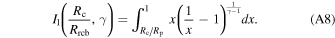
A natural outcome of atmospheric mass loss is that larger planetary cores at a cooler equilibrium temperature retain a larger atmospheric mass fraction due to their increased gravitational potential well and reduced irradiation. It is this basic result that introduces a slope in the radius-period valley rather than having a single radius that separates H/He-rich planets from stripped cores. Further, as we demonstrate in Figures 1 and 2, if one takes this simple fact into account, the mass–radius relation of planets that have undergone atmospheric escape naturally reproduces the observations. Here we demonstrate this analytically, as well as highlighting why this result holds for both photoevaporation and core-powered mass loss, emphasizing that both models agree with the exoplanet demographics because the underlying physics is similar. To analytically show that larger planetary cores at cooler equilibrium temperatures retain a larger atmospheric mass fraction, consider a planet with core mass Mc and radius Rc, equilibrium temperature Teq, hosting a H/He-dominated atmosphere. This atmosphere is split into a convective interior (assumed to be adiabatic with index γ) and a radiative exterior (assumed to be isothermal, with a temperature equal to Teq). The location of the radiative-convective boundary is Rrcb with density ρrcb. Following from Owen & Wu (2017), the mass of the convective interior scales as
where  is the Bondi radius for isothermal sound speed
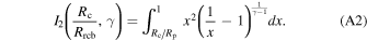
  . Here, I2 is a dimensionless integral that accounts for the mass distribution within the atmosphere:
In the case of hydrodynamic escape of planetary atmospheres, the mass-loss rate  scales as

where  is the Mach number of the escaping flow, evaluated at the radiative-convective boundary. For an isothermal outflow, the Mach number is only a function of RB/Rrcb and given by
where W0 is the real branch of the Lambert W function (see Cranmer 2004) and C is a constant. It is through this constant C that photoevaporation and core-powered mass loss distinguish themselves. This is because even in photoevaporation, the outflow is approximately isothermal between the radiative-convective boundary and XUV penetration point. Thus, the Mach number at the radiative-convective boundary is still given by a solution to the isothermal flow problem. However, unlike core-powered mass loss where the outflow is approximately isothermal all the way to the sonic point (and hence is the classic Parker wind solution; Parker 1958), in the photoevaporative case the outflow must typically supply a higher mass-loss rate to the XUV penetration point than provided by the Parker wind solution and is necessarily faster. Thus, in the case of XUV photoevaporation, C < −3 to provide these more powerful outflows, whereas for core-powered mass loss, C = −3 (see Lamers & Cassinelli 1999). For planets that have maintained a significant mass in H/He, i.e., sub-Neptunes, one can state that their mass-loss timescale  will be approximately constant. Hence, combining Equations (A1) and (A3), one finds that
This expression is dominated by the exponential term within  and only varies logarithmically with C, Rrcb and I2.
8
Thus, since the variation is only logarithmic with C, there is no leading order difference in the dependence on fundamental parameters between photoevaporation and core-powered mass loss.
9
Hence, one can state that
and only varies logarithmically with C, Rrcb and I2.
8
Thus, since the variation is only logarithmic with C, there is no leading order difference in the dependence on fundamental parameters between photoevaporation and core-powered mass loss.
9
Hence, one can state that
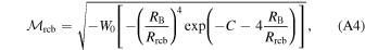
Now, by combining Equations (8), (9) and (11) from Owen & Wu (2017; see also Ginzburg et al. 2016), which assume radiative diffusion at the radiative-convective boundary for a cooling/Kelvin–Helmholtz timescale τKH, one finds that the density at the radiative-convective boundary scales as

where κ is the opacity and I1 is another dimensionless integral accounting for the binding energy of the planet:
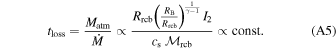
Combining the density at the radiative-convective boundary from Equation (A7) with the atmospheric mass from Equation (A1) and noting that RB/Rrcb is approximately constant from Equation (A6), one can show that
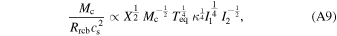
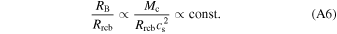
where the atmospheric mass fraction is defined as X ≡ Matm/Mc, and we have assumed that for a set of planets with the same age, their Kelvin–Helmholtz timescale will be approximately constant. Finally, recalling again that  is approximately constant from Equation (A6), one finds that

If one numerically evaluates the dimensionless integrals I1 and I2 (see Figure 11 from Owen & Wu 2017), one can show that  is approximately constant as a function of Rc/Rrcb. If one also assumes that the opacity κ is constant, then one finally finds that the atmospheric mass fraction of planets that have undergone mass-loss scales approximately linearly with core mass and inversely with the square root of equilibrium temperature. Moreover, this analytic argument is agnostic with respect to mass-loss models, i.e., photoevaporation versus core-powered mass loss. The main takeaway result is that larger-mass planets at cooler equilibrium temperatures will retain larger atmospheric mass fractions if they have undergone mass loss. This result is key to explaining the mass–radius distribution of exoplanets. Note, however, from Figure 2, that while final atmospheric mass fraction increases with core mass at a given equilibrium temperature, it is not a linear or even log-linear relation. This is the case when one fully evaluates the integrals of Equations (A2) and (A8) and takes nonconstant opacities into account, as is the case in the semianalytic models of Owen & Wu (2017), Owen & Campos Estrada (2020), Ginzburg et al. (2018), and Gupta & Schlichting (2019).
Footnotes
- 3
The term "core," as used for the remainder of this Letter, refers to the solid/liquid bulk interior of a planet, as opposed to the geological nomenclature of the iron core. In general, the mass of a sub-Neptune is approximately given by its core mass, as the atmospheric mass makes up less, often much less, than 10% of the planet's total mass.
- 4
We note that it remains unclear as to whether a 1:1 composition ratio would appear for condensation models that consider a realistic, evolving protoplanetary disk.
- 5
This is because the trend of entropy with mass is maintained across various ages, meaning that the slope and position of the mass–radius plane are age insensitive.
- 6
In fact, other literature values would place K2 18 b precisely on the mass–radius relations for H/He atmospheres and water worlds (e.g., Sarkis et al. 2018).
- 7
We also highlight that the bias of planet mass measurements is currently not quantifiable since such surveys are not based on homogeneous observations of a well-defined sample of stars.
- 8
This can be seen by Taylor expansion of the Lambert W function in the limit Rrcb/RB ≪ 1.
- 9
Note that while the scaling on fundamental parameters is the same, the normalization constant varies between the two models as photoevaporation drives more powerful outflows but for a shorter period of time.