Unified Picture of the Local Interstellar Magnetic Field from Voyager and IBEX

The interstellar medium (ISM) is composed of ionized and magnetized plasma, neutral gas, and dust that are remnants of ancient debris from fossil winds and exploded stars. Our Sun carves out a place in the midst of this material by continuously emitting a solar wind that expands supersonically outward in all directions and inflates a bubble known as the heliosphere (Parker 1961; Axford et al. 1963; Holzer 1972; Baranov et al.1976).

The Sun and its heliosphere move with respect to the nearby, or local, interstellar medium (LISM) at a speed of ∼26 km s⁻¹ (McComas et al. 2015), forming a highly asymmetric interaction. The direction of the heliosphere's motion through the LISM with respect to the local interstellar magnetic field (LISMF) forms a plane that organizes the interactions of interstellar material at the boundary (Izmodenov et al. 2005; Lallement et al. 2005; Pogorelov et al. 2008). The surrounding interstellar magnetic fields, plasmas, and charged particles press up against the solar material, forming a blunt nose, deflecting outward along the poles and flanks, and eventually stretching to form an elongated "heliotail" on the downwind side (e.g., Parker 1961; Wallis 1975; McComas et al. 2013, 2020 and references therein). This region of the ISM immediately surrounding the Sun is commonly referred to as the "very local interstellar medium" (VLISM).

Neutral atoms in the LISM (predominantly hydrogen) drift into the heliosphere unhindered by the magnetic field and plasma interactions. Some fraction of these get ionized and gain energy as they are swept outward with the solar wind, thereby forming the population of pickup ions (PUIs; Vasyliunas & Siscoe 1976; Hovestadt et al. 1985; Möbius et al. 1985; Isenberg 1986). These suprathermal PUIs carry substantial energy and dominate the thermal pressure of the bulk solar wind plasma beyond ∼20 au from the Sun and are expected to be preferentially accelerated at the solar wind termination shock (e.g., McComas et al. 2017a, 2021). Meanwhile, energetic neutral atoms (ENAs) are produced in the heliosheath—the subsonic-flowing, hot plasma region between the termination shock and the heliosphere's outermost boundary, the heliopause—via charge exchange between inflowing interstellar neutrals and the shock-energized PUIs (McComas et al. 2009a, 2011).

Over the last solar cycle, the two Voyager spacecraft have been directly sampling the plasma, magnetic field, and energetic particles in the heliosheath and VLISM. Voyager 1 crossed the heliopause boundary on 2012 August 25, at a radial distance of 121.6 au from the Sun, north of the ecliptic and ∼30° above the nose of the heliosphere at 2550 longitude and 350 latitude in solar ecliptic coordinates (Burlaga et al. 2013; Gurnett et al. 2013; Krimigis et al. 2013; Stone et al. 2013). Voyager 2 crossed six years later, on 2018 November 5, at a radial distance of 119.0 au, south of the ecliptic and toward the flank (2904 longitude and −322 latitude; Burlaga et al. 2019a; Gurnett & Kurth 2019; Krimigis et al. 2019; Richardson et al. 2019; Stone et al. 2019).

The signatures of the heliopause crossing were, at first, surprising and difficult to interpret. The energetic particles clearly showed a transition into a new region, signified by an abrupt (less than 1 day) increase in the intensity of cosmic rays coinciding with a sudden depletion of solar particles (Krimigis et al. 2013, 2019; Stone et al. 2013, 2019; Webber & McDonald 2013; see also review by Rankin et al. 2022 and references therein), implying a heliopause thickness of <5 × 10⁻³ au (Burlaga et al. 2019a). Meanwhile, the magnitude and variation of the magnetic field clearly changed from that of the weak, turbulent fields of the heliosheath (∼0.17 nT) to those of the stronger, smoother fields expected for the ISM (∼0.43 nT at Voyager 1; ∼0.68 nT at Voyager 2). However, the magnetic field direction observed at both spacecraft remained surprisingly consistent with that of the Parker spiral in the heliosheath, with a deflection of <5° at Voyager 1 and <10° at Voyager 2 (computed from 25 day averages before and after each crossing; see also Burlaga et al. 2013; Gurnett et al. 2013; Burlaga et al. 2019a).

An absence of direct plasma measurements required Voyager 1 to rely on other means for ascertaining the characteristics of the newly encountered VLISM. Radio emissions resulting from episodic electron plasma oscillations detected by the Plasma Wave Subsystem (PWS) revealed densities (∼0.08 cm⁻³) that were more consistent with the ISM, inferred from the scintillation of starlight (0.1 cm⁻³ expected) than the heliosheath (∼0.002 cm⁻³; Frisch et al. 2011; Gurnett et al. 2013; Gurnett & Kurth 2019). Other details about the plasma were later determined by the Voyager 2 plasma instrument (PLS). For example, combined data from PLS and PWS revealed that the plasma was hotter than expected—30,000–50,000 K observed versus 15,000–30,000 K predicted (Richardson et al. 2019).

Meanwhile, over much of the same time period, the Interstellar Boundary Explorer (IBEX; McComas et al. 2009a) provided continuous, global measurements of ENAs, which have led to a revolutionary, new understanding about the size, shape, and global characteristics of the heliosphere, the general properties of the LISM including its embedded magnetic field, as well as the dynamical interaction between them (see, e.g., McComas et al. 2017b, 2020 and references therein). IBEX's remote, energy-resolved, all-sky maps—covering an energy range of 0.1 to 6 keV—continue to yield groundbreaking results and discoveries (see, e.g., summary by McComas et al. 2017b). Perhaps foremost among these is the detection of an enigmatic ribbon of enhanced ENA emission that emanates from a narrow (∼20° wide in the 0.7–2.7 keV energy range; Fuselier et al. 2009), nearly circular region of the sky (Funsten et al. 2009, 2013) that is roughly a factor of 2–3 brighter (McComas et al. 2009b) than the surrounding, expected globally distributed flux, which arises largely from charge exchange in the heliosheath. The existence of the ribbon came as a complete surprise, and since its discovery in 2009 (Funsten et al. 2009; Fuselier et al. 2009; McComas et al. 2009b; Schwadron et al. 2009) over a dozen theories have emerged to explain its origin (see reviews by McComas et al. 2011, 2014; see also Giacalone & Jokipii 2015; Zirnstein et al. 2018a). The accumulated evidence so far most strongly supports some sort of "secondary ENA" process, which has the following key features: (1) some fraction of solar wind and heliosheath ions become neutralized and travel outward into the VLISM; (2) within several 100 au of the heliopause, many of these neutrals are reionized and gyrate around the local magnetic field; (3) within a few years (on average), these ions undergo a second charge exchange, thereby contributing to a population of secondary ENAs that travel back into the heliosphere and may be observed by IBEX from directions approximately perpendicular to the draped LISMF (e.g., McComas et al. 2009b; Schwadron et al. 2009; Chalov et al. 2010; Heerikhuisen et al. 2010; Schwadron & McComas 2013; Isenberg 2014; Giacalone & Jokipii 2015; Zirnstein et al. 2020; see also Table 1 of Zirnstein et al. 2015). Nevertheless, a complete understanding of the microphysical processes governing PUIs outside the heliopause before they become secondary ENAs has not yet been achieved and remains an active area of investigation.

An important clue concerning the origins of the IBEX ribbon resides in its location in the sky. More broadly, the ordering of the ribbon highlights the regions where the draped LISMF is perpendicular to the radial direction to the Sun (and nearly along IBEX's line of sight) and thereby demonstrates that the magnetohydrodynamic interaction of the heliosphere with the VLISM is intermediate between the magnetically and dynamically dominated extremes (McComas et al. 2009b; originally theorized by Parker 1961). Schwadron et al. (2009) hypothesized that the ribbon's center aligns with the direction of the LISMF and found the regions of the ribbon's highest fluxes to be remarkably well correlated with the direction perpendicular to the LISMF determined by a preexisting, Voyager-informed model (Pogorelov et al. 2009). Heerikhuisen & Pogorelov (2011) combined data from Voyager, SOHO, and IBEX with their computational heliospheric model and estimated the following parameters for the ISMF: magnitude = 0.2 to 0.3 nT, ecliptic longitude = 220° to 224°, and ecliptic latitude = 39° to 44°. Schwadron et al. (2015) showed that the field direction measured by Voyager 1 was >40° off from the center of the IBEX ribbon and the B − V plane, a plane of symmetry containing the LISMF and the LISM flow vector. Those authors used the extrapolated field to estimate the gradient scale size of the magnetic field and triangulate the direction of the LISMF. Soon after, Zirnstein et al. (2016) derived the pristine LISMF's magnitude and location far from the Sun (∼1000 au) by performing a chi-square minimization analysis between a global heliosphere model of the LISMF interaction with the heliosphere, ribbon ENAs produced from this interaction at each IBEX energy passband, and the IBEX data. They ascertained a field strength of 0.29 nT and direction of 227° and 346 in ecliptic longitude and latitude, respectively.

In the past decade, many studies have demonstrated the effectiveness of using IBEX ribbon data to constrain models of the magnitude and direction of the LISMF and also to inform how it drapes around the heliosphere (Grygorczuk et al. 2011; Heerikhuisen & Pogorelov 2011; Ratkiewicz et al. 2012; Heerikhuisen et al. 2014; Zirnstein et al. 2016). LISMF vectors derived from global heliosphere models have also been compared directly to Voyager data, both with (e.g., Pogorelov et al. 2021) and without (e.g., Izmodenov & Alexashov 2020) constraints from IBEX; it is the former which tend to show the most reasonable agreement. In addition to information supplied by IBEX, the impact of solar transients has also been shown to be important when we compare simulations of the draped LISM to Voyager observations; these time variations are particularly relevant for reproducing the smaller-scale structures, which are superimposed on the large-scale draped field (Kim et al. 2017; Pogorelov et al. 2021). At larger scales, simulations have found that the nature of the draping close to the heliopause, and its consistency or lack thereof with Voyager 1 and 2 measurements, is sensitive to the assumptions for the LISMF far from the heliosphere.

Here, we combine Voyager's two series of in situ magnetic field measurements with IBEX's global observations of the ribbon to present a unified picture of the LISMF from its draping around the heliopause to its unfolding into the pristine ISM. We directly compare magnetic field components observed locally at the two Voyager spacecraft to independently obtained results of the interstellar magnetic field from Zirnstein et al. (2016)'s best-fit IBEX ribbon model, extending from the heliopause out to ∼1000 au in the Voyager 1 and 2 directions. We show how these findings directly relate to the magnitude and direction of the unfolded LISMF inferred from the IBEX ribbon and discuss broader implications regarding the extent of the heliosphere's influence on its interstellar surroundings.

Figure 1 shows the direction and magnitude of the magnetic field encountered by Voyager 1 from its heliopause crossing at ∼121.6 au out to ∼155.0 au, extending a net distance of ∼33.4 au into the VLISM. In keeping with how the data are reported by the Voyager magnetometers, vectors are shown in the R, T, N spacecraft-centered coordinate system, for which $\hat{R}$ is the Sun-to-spacecraft vector; $\hat{T}$ is the cross product of the Sun's rotation vector (northward) with $\hat{R}$, so that $\hat{T}$ lies in the solar equatorial plane; and $\hat{N}$ completes the right-handed coordinate system. In this study, we show the components rather than angles to present a more complete picture of the Voyager measurements. Voyager 2 data are shown in Figure 2, covering a much shorter distance of ∼6.8 au beyond the heliopause (∼119.0 au out to ∼125.8 au) owing to the spacecraft's briefer time in the VLISM (from ∼2018.85 to ∼2021.01; using the most recent publicly available Voyager 2 data). As inferred from the Voyager termination-shock crossing location data and models (Opher et al. 2006; Pogorelov et al. 2007, 2011; Stone et al. 2008) and anticipated by IBEX (e.g., McComas & Schwadron 2014), the field strength in the Voyager 2 direction south of the ecliptic is significantly greater than at Voyager 1 in the north. The collective long-term trends indicate slowly varying and consistently changing field directions, with the components undraping more gradually at Voyager 1 than at Voyager 2. Burlaga et al. (2022) provided a numerical comparison of these effects, cast in terms of azimuth and elevation. They reported the values in units of yr⁻¹, but here we convert them to au⁻¹: −0786 ± 0002 au⁻¹ in azimuth (average of 280° ± 23°) and 0094 ± 0002 au⁻¹ in elevation (average of 23° ± 7°) at Voyager 1 and 31 ± 006 au⁻¹ in azimuth (average of 275° ± 7°) and 16 ± 006 au⁻¹ in elevation (average of 28° ± 5°) at Voyager 2.

Zoom In Zoom Out Reset image size

Zoom In Zoom Out Reset image size

Superimposed on these long-term trends are shorter variations that show pronounced structure (see, e.g., Figures 1(d) and 2(d)). In general, measurements by the two Voyagers reveal that the VLISM immediately surrounding the heliosphere is strongly influenced by the Sun and heliospheric processes. Such processes manifest through a variety of propagating transient phenomena measured locally at each spacecraft, including: cosmic-ray intensity enhancements (Gurnett et al. 2015, 2021b; Rankin et al. 2019b, 2020); electron plasma oscillations (Gurnett et al. 2013, 2021a; Gurnett & Kurth 2019; Ocker et al. 2021); weak, laminar shocks and "pressure front" waves (Burlaga & Ness 2016; Kim et al. 2017; Richardson et al. 2017; Burlaga et al. 2019b; Burlaga et al. 2021, Burlaga et al. 2022); and long-duration, pitch-angle dependent episodes of cosmic-ray intensity depletion, commonly referred to as "cosmic ray anisotropies" (Krimigis et al. 2013; Rankin et al. 2019b, 2020; Nikoukar et al. 2022; Rankin et al. 2022). The perturbations in the magnetic field seen in Figures 1 and 2 are characterized by sudden enhancements, followed by gradual decays, which deviate from nominal values; those with cosmic ray and electron plasma precursors are typically classified as shocks ("sh"), while those without such events are often referred to as waves, or pressure fronts ("pf"). Onset times for such events are also denoted in Figures 1 and 2 (blue solid lines) and labeled according to their identification by Burlaga et al. (2022).

Overlaid on the data are the results from Zirnstein et al. (2016)'s self-consistent simulation (solid green lines), based on fitting a secondary ENA source for the IBEX ribbon data measured at multiple energies. An important aspect of this model is that it did not use Voyager observations in any way, except by constraining the heliopause boundary distance so that it approximately reproduced the distance of Voyager 1's crossing at 121.6 au. ⁶  The simulation performed a chi-square minimization analysis to find the LISMF far from the heliosphere's influence (∼1000 au) that, once draped around the heliosphere, yielded a model of the ribbon that best fit IBEX-Hi data over ESA steps 2–6. In this study, we show simulation results from Table 1, Case 4 of Zirnstein et al. (2016): the interstellar boundary conditions were applied at a radius of 1000 au from the Sun and used a proton density of 0.09 cm⁻³, hydrogen density of 0.154 cm⁻³, temperature of 7500K, and a magnetic field of 0.3 nT pointing in a direction of 22699 longitude, 3482 latitude in ecliptic J2000 coordinates—close to the best-fit results from the minimization process. LISM speed, temperature, and inflow direction were obtained from IBEX helium observations (see McComas et al. 2015 and references therein). Solar wind conditions were based on long-term averages observed in the solar wind during the time period of 2000–2012 (e.g., Sokół et al. 2013), with 1 au parameter set to proton density = 5.74 cm⁻³, temperature = 51,100 K, speed = 450 km s⁻¹, and radial magnetic field = 3.75 nT, with a 45° angle of the field in the R–T plane. To avoid an artificially flat current sheet in the solar wind, the same polarity magnetic field was used in both the northern and southern hemispheres at the inner boundary. The VLISM magnetic field, plasma, and neutral densities were carefully chosen and balanced against each other (Heerikhuisen et al. 2014) to produce (i) the observed hydrogen density inside the heliosphere known at the time (see Swaczyna et al. 2020), (ii) the observed distance to the heliopause, and (iii) the observed IBEX ribbon geometry.

Zirnstein et al. (2016) performed a careful analysis of the IBEX ribbon produced by various magnetic field configurations and determined the optimum field strength and orientation by matching the simulation of the ribbon to the enhanced ENA flux seen in the IBEX data. Hence, the interstellar magnetic field in the simulation is derived solely from IBEX data. For this reason, it is interesting to compare this field with that observed by the Voyager spacecraft. An initial comparison was made by Zirnstein et al. (2016), in their Table 2, to Voyager 1 observations averaged over 2012.8–2014.6, suggesting initial agreement with Voyager 1. After the Zirnstein et al. (2016) model was developed, Swaczyna et al. (2020) found the interstellar neutral hydrogen density extrapolated to the termination shock using New Horizons SWAP observations of interstellar PUI to be 40% higher than previously thought. To "rebalance" the modeled pressure in the heliosphere, the plasma and neutral densities have since been updated from the original values used by the Zirnstein et al. (2016) model in order to be consistent with items (i) and (ii) described above (e.g., Zirnstein et al. 2022). However, the VLISM magnetic field parameters remain unchanged because they are separately constrained by the IBEX data, and any change to the magnetic field would cause the modeled ribbon to disagree with IBEX observations. Therefore, the LISMF results from Zirnstein et al. (2016) remain applicable here.

Figure 1 shows that the IBEX-derived model is remarkably consistent with the Voyager 1 data out to 30 au beyond heliopause. Likewise, the model strongly agrees with the observations of B _t and B _n accumulated so far from Voyager 2, which is on an entirely different trajectory (albeit with much shorter distance beyond the heliopause) compared to its twin (Figure 2). The large-scale, gradual trends highlighted by the IBEX-constrained model results provide an interesting context for the fine-scale perturbations observed locally by the Voyagers. As described earlier, the fine-scale perturbations are associated with shocks and pressure waves generated by transient events that originate from within the heliosphere and survive out to the heliopause boundary where they partially reflect back into the heliosheath and partially transmit across the heliopause (e.g., Richardson et al. 2017; McComas et al. 2018b; Zirnstein et al. 2018b; Rankin et al. 2019a). These structures are not included in the steady-state heliosphere model from Zirnstein et al. (2016), which shows the large-scale undraping of the field.

The component that shows the least agreement between the data and model is B _r (Figures 1(a) and 2(a)). While no model is infallible, it is difficult to explain how a singular component of a vector derived could be off in a way that leaves the other components unaffected. Instead, we find it more likely that the issue in B _r is related to the data for several reasons, including (1) it points along the spacecraft-to-Sun direction vector, which makes it the most difficult to calibrate since this direction must be continually maintained (whereas the other components are regularly calibrated via spacecraft repointing maneuvers); (2) it is the weakest in magnitude and therefore much nearer to the limit of the instrument's detection capabilities; (3) the uncertainties above (Figures 1 and 2), as reported in the publicly available data, were adopted in the early phase of the mission and are probably not realistic for the VLISM; (4) the observed trend of B _r at Voyager 1 toward zero and possibly negative values and the positive trend of B _r at Voyager 2 imply an undraping of a field that is not only inconsistent with the IBEX Ribbon but cannot physically persist since it must converge to the same direction far from the heliosphere (see Figure 3); and (5) the primary method of calibrating B _r outside the heliopause is by the "compression assumption" (see Berdichevsky 2009, page 4). It was confirmed by the Voyager team that this is the primary method of calibrating B _r outside the heliopause.

Zoom In Zoom Out Reset image size

The compression assumption (item (5) above) relies on the assumption that if ΔB_x /B_x = ΔB_y/B_y = α, where B _x and B _y are the transverse components, then it must mean ΔB_x/B_x = ΔB_y/B_y = ΔB_z/B_z = α, where B _z is the radial component. Using this assumption, the calibration of B _z is based on measurements of B _x and B _y before and after the compression, allowing the determination of B _z using the inboard and outboard field measurements (see details in Berdichevsky2015). However, it is flawed to assume that ΔB_x/B_x = ΔB_y/B_y = ΔB_z/B_z is always true, primarily because shocks/compressions outside the heliopause—which are most often quasiperpendicular—do not in fact compress B _z (the component normal to the shock) the same way as B _x and B _y. Therefore, the derived value for B _z would be underestimated (overestimated) if the compression in the radial direction is more (less) than the B _x and B _y components. This latter point may be the most significant reason for questioning the current method for calibrating B _r, which can lead to an incorrectly updated value each time the compression assumption is used. This also seems supported by the fact that the model and data compare reasonably well just outside the heliopause for all components but then gets worse over time for B_r.

While it is always possible that there may be some very thick boundary (>30 au) beyond the heliopause (e.g., Fisk & Gloekler 2022), in this study we follow the more widely accepted notion that the Voyagers are beyond such a structure and that the VLISM field is, on average, naturally undraping as the spacecraft move further out (as shown in the simulations of, e. g., Izmodenov & Alexashov 2020; Opher et al. 2020; Kornbleuth et al. 2021; Pogorelov et al. 2021; Zirnstein et al. 2021 and references therein; see also, e.g., review by Kleimann et al. 2022). Sufficiently far from the heliosphere, magnetic field vectors measured at any point in the VLISM must undrape to the same direction. This is demonstrated by the modeled LISMF derived from the IBEX ribbon, shown as colored circles in Figure 3. When projected onto a sky map in a common coordinate system (here we choose ecliptic J2000), the modeled LISMF in the direction of each spacecraft ( B ${}_{{\rm{V}}1,\mathrm{mod}}$, B ${}_{{\rm{V}}2,\mathrm{mod}}$) unfolds into the common pristine LISMF vector far from the heliosphere ( B @1000 au; magenta star). In contrast, the Voyager observations (colored cross symbols; also in ecliptic J2000) show trends that are inconsistent, both with the modeled undraped LISMF and with each other. For example, Voyager 1's total field vector moves toward the starboard side of the heliosphere, nearly 90° away from the trajectory of Voyager 1 itself. This trend is directly related to the behavior of the B _r component in Figure 1, which shows B _r decreasing to ∼0 nT after ∼135 au from the Sun. Meanwhile, Voyager 2's magnetic field vector unfolds in the opposite direction; this is also linked to B _r, which, as shown in Figure 2, continues to increase as a function of distance from the heliopause, and thus the field vector trends toward the direction of Voyager 2's trajectory. The susceptibility of this component is further demonstrated as follows: if we replace the Voyagers' measured B _r values with those from the model (leaving B _t and B _n unchanged), the large-scale trends become much more consistent between the two spacecraft, the model, and the ultimate direction of the pristine LISMF, as demonstrated in the right panel of Figure 3. This is not by any means an argument to discard the data and replace it with a model. Rather, it is a demonstration of the fact that, regardless of what the explanation might be, the magnetic field must eventually undrape, and the VLISM magnetic field vectors measured by the two spacecraft must eventually agree, but this is currently not the case, and the instigator is the B _r component.

In general, the calibration of the magnetometers is a very difficult task. As these results confirm, the calibration works remarkably well for B _t and B _n, which were designed to be calibrated using inputs from spacecraft spinning maneuvers (e.g., magnetometer roll maneuvers, or "MAGROLs"). However, the off pointing cannot be performed for B _r. Instead, the Voyager magnetometers attempt to calibrate B _r with respect to the average expected value for the Parker spiral (Berdichevsky 2009), an approach which breaks down outside the heliosphere, where less robust methods (Berdichevsky 2015) had to be employed. Therefore, based on the results of this analysis, a clear need to update the uncertainties from values reported since early on in the mission, and the fact that the large-scale trend of the LISMF must approach the same direction as measured from any vantage point in the sky far from the heliosphere, we conclude that the B _r component derived from Voyager 1 and Voyager 2 measurements is questionable and in its present form, should not be included in analyses of the large-scale LISMF. Beyond this, our analysis confirms that the large-scale undraping of the LISMF determined by the IBEX ribbon measurements (Zirnstein et al. 2016) agrees very well with the observations of the transverse components from Voyager 1 and 2.

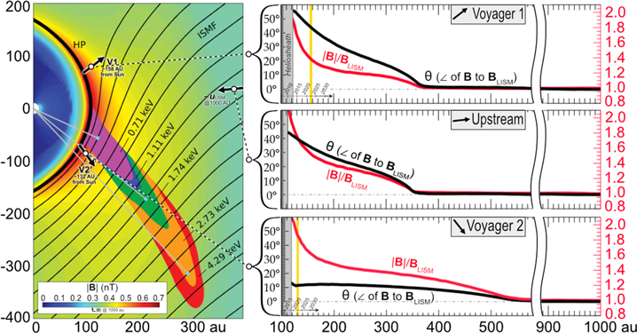
Figure 4 provides a global picture of the LISMF from its draping around the heliopause out to the "pristine" ISM, which is taken to be at 1000 au (McComas et al. 2015). The left side shows the magnitude (background multicolored shading) and direction (black curves) of the LISMF as it approaches the heliopause, as determined from the model of the IBEX ribbon (viewed from the meridional plane), with arrows to roughly indicate the Voyager 1 (V1), Voyager 2 (V2), and plasma inflow (u_LISM) directions projected onto the plane (adapted from Zirnstein et al. 2016). The right-hand panels show cuts along the Voyager 1 and 2 trajectories (top and bottom panels), as well as in the upstream (nose) direction of the heliosphere (opposite to the direction of interstellar inflow; middle panel). An important question to address is: how far must each spacecraft travel before it encounters the unfolded LISMF inferred from the IBEX ribbon? This was investigated by comparing how the LISMF magnitude (∣ B ∣) and direction (θ) behave with respect to the values at 1000 au ( B _LISM).

Zoom In Zoom Out Reset image size

At the time of this writing (∼2022.75), Voyager 1 is at a distance of ∼158 au from the Sun, and the field points 44° away from the direction of the unfolded LISMF. Its magnitude is 38% greater than that of the LISMF. Although the field is less draped in the Voyager 2 direction, it is also more compressed, with an offset of 12° and 84% greater magnitude at ∼132 au. As shown in the top right panel of Figure 4, a large gradient occurs along the Voyager 1 direction from the heliopause up until ∼366 au, where the angle comes to within 3° of the LISMF and the magnitude comes to within 1.5%. Given the spacecraft's speed of ∼3.6 au yr⁻¹ it will take ∼58 more years for Voyager 1 to reach this region, far beyond its operational timeline. In the Voyager 2 direction (Figure 4, bottom right panel), the magnetic field progresses more slowly, and it is not until ∼513 au from the Sun that the magnetic field has unfolded to within 3° and 7.1% of that of the pristine LISMF. At its speed of ∼3.3 au yr⁻¹ it would take Voyager 2 another ∼115 years to observe this. More practically, should the twin spacecraft continue to operate for another decade, the model predicts that the Voyager 1 magnetic field will have unfolded to within 34° and weakened in magnitude to within 26% of the LISMF value, and the Voyager 2 field should unfold to within 12° but still remain much larger in magnitude (205% of the LISMF value) at a radial distance of 165 au. As these figures demonstrate, the behavior of the magnetic field just beyond the heliopause can vary significantly depending on spacecraft trajectory, the implications of which should be considered for future interstellar missions. For example, preliminary analysis using the IBEX model suggests that the VLISM field near the heliopause most closely resembles the LISMF on the port side, toward the flank.

In conclusion, this study provides important insight into the behavior of the LISMF, from how it drapes around the heliopause to how it unfolds into the pristine ISM, through combined perspectives from IBEX and Voyager. We have demonstrated that using the components rather than angles presents a much clearer picture of the Voyager measurements and that the transverse components of the VLISM field measured by the Voyagers agree very well with values predicted by IBEX. However, we have also identified a clear discrepancy between the model and observations, as well as between the two sets of Voyager measurements, in the radial component. Because of this component, the continual observational trends do not lead to a single field direction far from the heliosphere, despite the fact that they must eventually converge. It is recommended that these issues be further investigated and that more realistic uncertainties be defined for the publicly released magnetic field data or even that a better method be constructed for calibrating B _r. Related to the large-scale structure of the LISMF, we have provided predictions on how the field should continue to undrape along the two Voyager directions and argue that the best values to use for the magnitude and location of the pristine ISM field (∼1000 au) are those independently derived from the IBEX ribbon: a field strength of 0.29 nT and direction of 227° in ecliptic longitude and 346 in ecliptic latitude (from Zirnstein et al. 2016). The findings here provide but one example of how, despite differing sets of instrumentation, complimentary Voyager and IBEX observations can lead to a more unified picture of the global heliosphere and its surroundings. We look forward to seeing how future studies and missions such as IMAP (McComas et al. 2018a) utilize the effective combination of in situ and global observations to further our understanding about our place among the stars.

We are grateful to the many individuals who have contributed to making the IBEX and Voyager missions a success. This work was partially funded by the IBEX mission as part of the NASA Explorer Program (80NSSC20K0719) and the IMAP mission as a part of NASA's Solar Terrestrial Probes (STP) mission line (80GSFC19C0027). J.S.R. was supported by the NASA Early Career Investigator Program (ECIP), award number 80NSSC21K0456. E.J.Z. was supported by the NASA Outer Heliosphere Guest Investigator (OHGI) program, award number 80NSSC20K0783.