


Abstract
We report the discovery of the unusually bright long-duration gamma-ray burst (GRB), GRB 221009A, as observed by the Neil Gehrels Swift Observatory (Swift), Monitor of All-sky X-ray Image, and Neutron Star Interior Composition Explorer Mission. This energetic GRB was located relatively nearby (z = 0.151), allowing for sustained observations of the afterglow. The large X-ray luminosity and low Galactic latitude (b = 4 3) make GRB 221009A a powerful probe of dust in the Milky Way. Using echo tomography, we map the line-of-sight dust distribution and find evidence for significant column densities at large distances (≳10 kpc). We present analysis of the light curves and spectra at X-ray and UV–optical wavelengths, and find that the X-ray afterglow of GRB 221009A is more than an order of magnitude brighter at T0 + 4.5 ks than that from any previous GRB observed by Swift. In its rest frame, GRB 221009A is at the high end of the afterglow luminosity distribution, but not uniquely so. In a simulation of randomly generated bursts, only 1 in 104 long GRBs were as energetic as GRB 221009A; such a large Eγ,iso implies a narrow jet structure, but the afterglow light curve is inconsistent with simple top-hat jet models. Using the sample of Swift GRBs with redshifts, we estimate that GRBs as energetic and nearby as GRB 221009A occur at a rate of ≲1 per 1000 yr—making this a truly remarkable opportunity unlikely to be repeated in our lifetime.
Export citation and abstract BibTeX RIS

Original content from this work may be used under the terms of the Creative Commons Attribution 4.0 licence. Any further distribution of this work must maintain attribution to the author(s) and the title of the work, journal citation and DOI.
1. Introduction
Massive stars exhibit a broad continuum of properties in their terminal explosions. At one end are the cosmological long-duration gamma-ray bursts (GRBs), capable of coupling tremendous energies (≳1051 erg) to highly collimated ejecta with a bulk Lorentz factor Γ0 ≳ 100 (Piran 2004). On the other end, the energy budget of most stripped-envelope core-collapse supernovae is dominated by the (quasi)-isotropic supernova emission, with photospheric velocities of tens of thousands of kilometers per second (e.g., Liu et al. 2016). Intermediate between these two extremes lies the growing class of low-luminosity GRBs and relativistic supernovae (e.g., Margutti et al. 2014). Typified by the prototypical low-luminosity GRB 980425 associated with SN 1998bw (Galama et al. 1998; Kulkarni et al. 1998), these sources couple several orders of magnitude less energy to their moderately relativistic ejecta (∼1048 erg), and lack the high degree of collimation of cosmological GRBs.
In the nearby universe (z ≲ 0.3), where high-energy facilities are sensitive to low-luminosity GRBs, high-luminosity GRBs are exceedingly rare due to their much lower volumetric rate. Yet an energetic GRB observed within this volume could produce unprecedented brightness. Here we report the discovery of GRB 221009A, an extremely luminous GRB (Kann & Agui Fernandez 2022) in our cosmic backyard.
On 2022 October 9 at 14:10:17 UT, the Burst Alert Telescope (BAT; Barthelmy et al. 2005), on board the Neil Gehrels Swift Observatory (Swift; Gehrels et al. 2004), triggered twice in rapid succession on a new cosmic source in the constellation Sagitta. Following its automated burst response, Swift promptly slewed to the location of the first trigger, detecting a bright transient seen with both the Swift X-Ray Telescope (XRT; Burrows et al. 2005) and the Ultraviolet/Optical Telescope (UVOT; Roming et al. 2005). Due to the rarity of such a repeated BAT image trigger and the proximity of the source to the Galactic plane (b = 43), it was initially classified as a new Galactic X-ray and optical transient, and therefore was designated Swift J1931.1+1946 (Dichiara et al. 2022). Monitor of All-sky X-ray Image (MAXI; Matsuoka et al. 2009) reported the detection of bright X-ray emission from this location shortly thereafter (Negoro et al.2022).
Subsequently the Gamma-ray Burst Monitor (GBM; Meegan et al. 2009) on board Fermi reported the detection of an exceptionally bright long-duration GRB ≈55 minutes prior to the initial BAT trigger, with a consistent localization (Veres et al. 2022). Due to issues in receiving data, the automated classification and localization notices associated with this onboard GBM trigger were not distributed to the world. However, the Fermi team rapidly communicated the existence of the GBM trigger, and its spatial coincidence with the double BAT trigger, to the Swift team. This spatial association, together with analysis of prompt XRT data that showed a smooth GRB-like power-law decline, led to the conclusion that Swift J1931.1+1946 was in fact a GRB, GRB 221009A (Kennea et al. 2022). For the first time in the ∼18 yr since launch, BAT triggered not on the GRB prompt emission, but instead on the bright high-energy afterglow when GRB 221009A entered the field of view.
The unusual brightness of GRB 221009A prompted widespread follow-up at multiple wavelengths. Additional X-ray detections were reported by the Neutron Star Interior Composition Explorer (NICER; Iwakiri et al. 2022) and the Nuclear Spectroscopic Telescope Array (NuSTAR; Brethauer et al. 2022). The Large High Altitude Air Shower Observatory reported detecting photons up to 18 TeV (Huang et al. 2022). Changes in the strength of signals propagated by radio transmitters were recorded at the time of the GBM trigger as the photons from the GRB ionized Earth's atmosphere (Guha & Nicholson 2022; Schnoor et al. 2022). Spectroscopic observations of the afterglow and the host galaxy provided a redshift of z = 0.151 (Castro-Tirado et al. 2022; de Ugarte Postigo et al. 2022; Izzo et al. 2022), corresponding to a distance of 749.3 Mpc.
This paper is organized as follows: Section 2 contains analysis of the observations taken by Swift (BAT, XRT, and UVOT), MAXI, and NICER; in Section 3, we present analysis of the dust scattering echo, broadband spectrum, and light curve of the burst afterglow; we discuss how GRB 221009A compares to other GRBs in Section 4, investigate the astrophysical rate of similar events, and the nature of energetic GRBs; in Section 5, we present our conclusions. We show that due to the combination of proximity and large (but not unprecedented) intrinsic luminosity GRB 221009A has a much brighter X-ray afterglow than those of previously observed Swift GRBs, and such luminous nearby events are extremely rare occurrences.
For this paper, we assume a cosmology with H0 = 67.36, Ωm = 0.3153, Ωv = 0.6847 (Planck Collaboration et al. 2020), and z = 0.151 unless otherwise stated. We adopt the GBM trigger time as the burst onset, i.e., T0 = 13:16:59.99 UTC on 2022 October 9. Magnitudes are reported on the Vega system, and uncertainties are given at a 90% confidence interval (unless otherwise noted).
2. Observations
2.1. Swift Burst Alert Telescope
Figure 1 shows the BAT raw light curves (i.e., not background subtracted), summed over all detectors, from T0 − 500 s to T0 + 5000 s. The location of GRB 221009A was occulted by the Earth until T0 + 1870 s. At ∼T0 + 1100 s, the overall count rate began to rise due to increased particle background as Swift approached the South Atlantic Anomaly (SAA). From T0 + 1317–2183 s, BAT data collection was disabled as Swift transited the SAA. The count rate remained elevated while exiting the SAA until the spacecraft slew beginning at T0 + 2496 s, when we attribute the linearly decaying enhanced count rate to emission from GRB 221009A. However, the source location was not in the coded portion of the BAT field of view until a slew beginning at T0 + 3095 s.

Figure 1. BAT raw light curve from the rate data. Panel (a) shows the raw light curve in the 15–350 keV band with a time binning of 1.6 s. This light curve was made from BAT quad-rate data, which records continuous count rates from all active detectors in four different energy ranges (15–25, 25–50, 50–100, and 100–350 keV). The time period when the GRB was occulted by the Earth (within 69° of the Earth center) is marked in green. Spacecraft slew times are marked in gray. The two BAT trigger times are marked by red lines. Panel (b) shows the partial coding fraction as a function of time. A partial coding fraction of 0 indicates that the GRB was outside of the BAT coded field of view, and a value of 1 indicates that the source is in the highest sensitivity region of the BAT coded field of view.
Download figure:
Standard image High-resolution imageFinally after this slew completed, BAT triggered on GRB 221009A, at 14:10:18 (T0 + 3199 s; trigger ID 1126853) and 14:17:06 (T0 + 3607 s; trigger ID 1126854) UTC. The event data from these two triggers cover a time range from T0 + 2960 s to T0 + 4570 s. The mask-weighted light curve shows steadily declining emission present when the burst location came into the BAT field of view at T0 + 3173 s, and extending beyond the available event data range. The time-averaged spectrum from T0 + 3302 s to T0 + 4538 s is best fit by a simple power-law model, with Γ = 2.08 ± 0.03. The fluence in the 15–150 keV band is (7.4 ± 0.1) × 10−5 erg cm−2.
The smooth temporal evolution observed by BAT, together with the large temporal offset between the BAT and GBM triggers, indicates that BAT triggered on the afterglow of GRB 221009A. This marks the first such occurrence of a BAT afterglow trigger in the 18 yr of Swift operations.
Given the exceptionally bright afterglow, we searched for even later emission in the BAT survey mode data using the BatAnalysis Python package (T. Parsotan et al. 2023, in preparation). In individual pointings of survey mode data, the afterglow was detected until 2022 October 9 21:55:38 UT (T0 + 31 ks). We attempted to fit the spectra of each survey data set with a power-law (cflux*po) model in XSPEC (Arnaud 1996) to obtain fluxes and photon indices. Nondetections were then analyzed to obtain 5σ upper limits following the procedure outlined in Laha et al. (2022).
At later times, the survey data were binned daily and then mosaiced together. The spectrum from each mosaiced image was fitted, and the flux and photon indices were derived similar to the procedure above. The results of this analysis are plotted in the top panel of Figure 2, and listed in Appendix A.

Figure 2. Combined X-ray and UV–optical light curve of GRB 221009A. The upper panel shows observed X-ray flux from MAXI, NICER, XRT (all 0.3–10.0 keV), and BAT (14–195 keV). BAT data are taken from detections of the afterglow in Survey data; note that the final BAT data point combines all observations integrated over 1 day. The dotted line shows a broken power-law fit to the MAXI, NICER, and XRT data. The inset figure shows the first MAXI, BAT, and XRT data, with the black dashed line indicating a fit to the XRT data alone, and red dashed line a fit between the first MAXI point and the first XRT detection. The lower panel shows 7 filter optical and UV data from UVOT as obtained after the subtraction of late-time template images. The dashed line shows a power-law fit to the white band data.
Download figure:
Standard image High-resolution image2.2. Swift X-Ray Telescope
The XRT began observing GRB 221009A at 14:13:09 UT (T0 + 3370 s, 170 s after the first BAT trigger) and located a bright afterglow in the initial 0.1 s image-mode exposure, after which observations began in windowed timing (WT) mode. The initial WT count rate was 910 ± 40 ct s−1 (all XRT count rates are corrected for the effects of pile-up and hot columns; see, e.g., Evans et al. 2007); making it more than an order of magnitude brighter at this time—in observed flux—than any other GRB observed by XRT. Due to the high count rate, the XRT remained initially in WT mode, in which only 1D spatial information is collected. Significant structures are present in the 1D spatial profiles, with a clear excess compared to the expected point-spread function (PSF), which were evolving with time (see Appendix B). This resembles the behavior expected when dust clouds in our Galaxy scatter X-rays from the GRB prompt emission, which were not initially traveling toward Earth, back into our line of sight.
At T0 + 89 ks, the GRB had faded sufficiently that the XRT automatically switched to photon counting (PC) mode. The 2D image from this observation, shown in Figure 3, confirmed the presence of a complex series of expanding, bright rings associated with a dust-scattering echo (see also Tiengo et al. 2022; Vasilopoulos et al. 2023), the properties of which are discussed in Section 3.1.
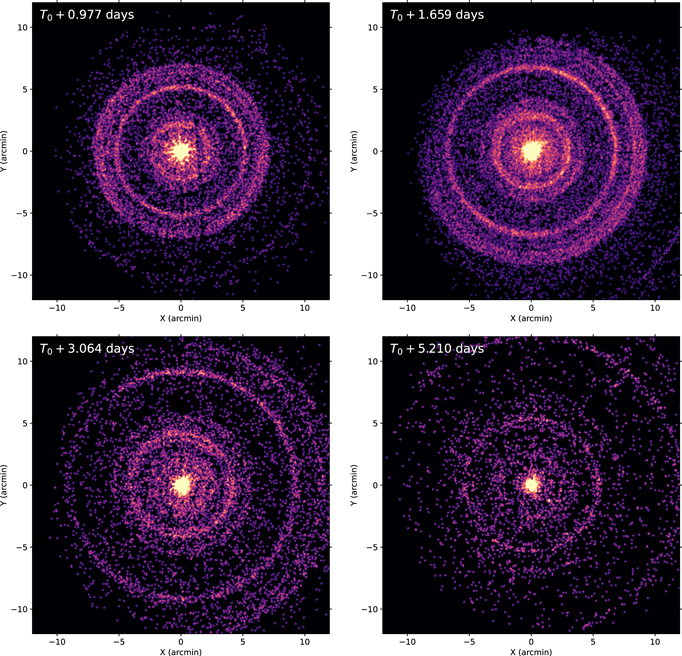
Figure 3. XRT PC-mode 0.8–5.0 keV images from ObsIDs 01126853004 (top left), 01126853006 (top right), 01126853008/09 (bottom left), and 01126853010/11 (bottom right), illustrating the echo expansion with time. The echo event radial positions were scaled by t−0.5 to each observation midtime (given in the upper left corner of each image in days since GBM trigger) to counter the halo expansion within each observation.
Download figure:
Standard image High-resolution imageThe presence of scattered emission complicates the data analysis, as it can contribute events to the regions over which source and background counts are accumulated. Both the intensity and spectrum of the rings are spatially variable; thus the selected background region may in fact not be representative of the background within the source region. As a result, the automated XRT analysis (Evans et al. 2007, 2009) needs some modification. For PC mode, this is relatively simple, as we have full 2D imaging, and the innermost rings were reasonably well separated from the GRB itself. We restricted the source region to a radius of 20 pixels (47''), and extracted a combined background from four regions 37 across the detector, which are as free from dust contamination as possible (identified from a stacked image of all PC-mode data). In order to quantify the impact of dust contamination in the background, we calculated the background rate in these regions, and found an average value of 1.6 × 10⁻⁶ ct s−1, which is consistent with historical values (Evans et al. 2023). During the first ∼5 days, dust ring contamination caused a 4–10 times elevation of the background rate. However, during this period, the afterglow of GRB 221009A is 30–50 times brighter than the background level, meaning the effect is negligible.
For WT mode, this is more problematic since the CCD is read out in columns, rather than pixels. After investigating the variation in the echo contribution to WT-mode data, we modified the default WT extraction regions to minimize its impact (see Appendix B). We found that the WT flux is accurate to ∼6%. We further verified this by extracting a light curve using only data above 4 keV, where dust scattering becomes less efficient, given the roughly ν−2 dependence of the scattering cross section; only minimal changes in the light-curve shape are observed. On the other hand, the dust has more significant impact on the WT spectra (Appendix B), resulting in an increase in the best-fit photon index up to ∼7% and a significant increase to the best-fit absorption column (up to ∼27%).
We modified the settings for the automated light curve 38 to limit the source extraction region to 20 pixels radius, and to use the PC-mode background region (described in the Appendix B); due to the unusual brightness of the source, we also increased the number of counts per bin by a factor of 10 compared to the default (see Evans et al. 2007 for details). We fit the time-averaged PC-mode spectrum using XSPEC with a power-law model and two absorption components. The first of these was a tbabs fixed to the Galactic value of 5.38 × 1021 cm−2 (Willingale et al. 2013); the second was a ztbabs with NH free and redshift fixed at 0.151. 39 The fit yields NH = (1.4 ± 0.4) × 1022 cm−2, with a photon index Γ = 1.8 ± 0.2. We used these results to convert the light curve into observed 0.3–10 keV flux. The resulting flux measurements are shown in Figure 2.
To investigate possible spectral evolution, we extracted a series of time-resolved spectra using the "Add time-sliced spectrum" option on the UKSSDC website 40 (Evans et al. 2009), which ensures that the modifications to the default processing parameters, described above, are employed. From the WT-mode data, we created one spectrum from the first spacecraft orbit (T0 + 3.4–4.5 ks), and then spectra in 10 ks chunks from T0 + 10–50 ks. For PC mode, we extracted spectra over the intervals T0 + 67–200, 200–400, 400–1000, and >1000 ks. For WT mode, we used only grade 0 events, as is recommended for very absorbed objects. 41 We fitted these spectra independently with the model defined above; the results are shown in Table 1. The photon index ranges between ∼1.6 and ∼1.9 with the harder profiles observed during the first block of observations (from 3.4 to 4.5 ks) and around 1–2 days (from 68 to 175 ks) after T0.
Table 1. Spectral Parameters Determined from Fitting a Power-law Model to the Time-resolved X-Ray Data from Swift, MAXI, and NICER
| T − T0 | Exposure | Intrinsic NH | Photon Index | Fit Stat./d.o.f. | Observatory/Detector |
|---|---|---|---|---|---|
| (ks) | (ks) | (1022 cm−2) | |||
| 2.5 | 0.047 | ⋯ | 1.75 ± 0.09 | 307/322 | MAXI/GSC |
| 3.4–4.5 | 1.2 | 1.28 ± 0.04 | 1.61 ± 0.02 | 1249/959 | XRT/WT |
| 8.0 | 0.047 | ⋯ |

| 145/166 | MAXI/GSC |
| 10.0–20.0 | 0.5 | 1.39 ± 0.09 | 1.89 ± 0.05 | 859/840 | XRT/WT |
| 14.0 | 0.029 | ⋯ | 1.89 ± 0.16 | 26.9/35 | NICER/XTI |
| 19.5 | 0.062 | ⋯ | 1.84 ± 0.15 | 23.6/36 | NICER/XTI |
| 20.0–30.0 | 2.9 | 1.36 ± 0.05 |

| 995/922 | XRT/WT |
| 30.0–40.0 | 1.7 | 1.25 ± 0.07 | 1.85 ± 0.04 | 800/840 | XRT/WT |
| 40.0–50.0 | 2.8 | 1.20 ± 0.06 | 1.84 ± 0.03 | 875/873 | XRT/WT |
| 52.6–98.0 | 2.1 | ⋯ | 1.85 ± 0.07 | 131/153 | NICER/XTI |
| 68–175 | 17 |

| 1.65 ± 0.08 | 655/727 | XRT/PC |
| 103.0–198.0 | 6.5 | ⋯ | 1.79 ± + 0.06 | 144/168 | NICER/XTI |
| 203.3–360.5 | 9.8 | ⋯ | 1.61
| 94/94 | NICER/XTI |
| 216–394 | 12 |

| 1.80 ± 0.10 | 632/665 | XRT/PC |
| 404–954 | 26 | 1.20 ± 0.18 | 1.92 ± 0.10 | 501/622 | XRT/PC |
| 505.0–961.6 | 2.7 | ⋯ | 1.82 ± 0.19 | 58.1/67 | NICER/XTI |
| 1005–6285 | 0.24 | 1.00 ± 0.15 | 1.91 ± 0.09 | 723/668 | XRT/PC |
Note. NICER/XTI and MAXI/GSC data are fit in the energy ranges 4–10 and 4–20 keV, respectively, to avoid contamination from unresolved dust echo contamination, with intrinsic NH fixed to 1.29 × 1022 cm−2. XRT spectra are fit in the range 0.3–10 keV, allowing for measurement of intrinsic NH. Note that fit statistics are C-stat (Cash 1979) for MAXI and Swift data; NICER are χ2. Galactic NH is fixed to a value of 5.38 × 1021 cm−2 (Willingale et al. 2013).
Download table as: ASCIITypeset image
2.3. Swift Ultraviolet/Optical Telescope
The UVOT began settled observations of the field of GRB 221009A at 2022 October 9 14:13:17 UT, T0 + 3.4 ks (179 s after the first BAT trigger; Dichiara et al. 2022; Kuin et al. 2022). A nearby star, 5'' away from the GRB, contaminates the photometry when using the standard circular aperture of 5'' radius. In order to minimize the star's contribution to the measurement of the afterglow, we use a 2 5 aperture to extract source counts. To be consistent with the UVOT calibration, these count rates were then corrected to 5'' using the curve of growth contained in the calibration files. Background counts were extracted using two circular regions of radius 15'' located in source-free regions identified from stacked deep images in each filter. The count rates were obtained from the image lists using the Swift tool uvotsource.
As GRB 221009A fades, even using a small aperture, the contribution from the nearby star increases in dominance. In order to estimate the level of contamination, for each filter, we combined the late-time exposures between T0 + (3.4 × 10⁶) s and T0 + (4.4 × 10⁶) s. We extracted the count rate in the late combined exposures using the same 25 aperture and applied an aperture correction to 5''. These were subtracted from the source count rates to obtain the afterglow count rates. The afterglow count rates were converted to magnitudes using the UVOT photometric zero-points (Poole et al. 2008; Breeveld et al. 2011), as well as to fluxes. To improve the signal-to-noise ratio (S/N), the count rates in each filter were binned using Δt/t = 0.2. The final photometry is plotted in the bottom panel of Figure 2 and listed in Appendix C. We caution that the photometry in the uvw1 and uvw2 is likely impacted by red leak; see Siegel et al. (2014), Brown et al. (2010) for additional details.
2.4. MAXI
MAXI, which is on board the International Space Station (ISS), performs scanning observations of about 80% of the sky every 92 minutes. Prior to the GBM detection of the prompt emission from GRB 221009A, the two gas slit camera (GSC; Mihara et al. 2011) units, GSC_4 and GSC_5, scanned the source region at 12:25 UT on 2022 October 9 (T0−3.1 ks), and no enhancement was seen at that time. The 2–10 keV 3σ upper limit is 0.074 ct cm−2 s−1, corresponding to a flux of approximately 7.9 × 10⁻¹⁰ erg cm−2 s−1. At 13:58 UT (T0+2.5 ks) the GSCs detected a very bright transient with a 2–10 keV flux of 5.97 ± 0.19 ct cm−2 s−1 (∼6.5 × 10⁻⁸ erg cm−2 s−1; Negoro et al. 2022). Unfortunately, at the time the data were collected, there was a loss of the signal to the ground, and the data were stored in the High Rate Communication Outage Recorder in the ISS, leading to a delay in reporting the transient. Before downloading these stored data at around 15:55 UT, the MAXI/GSC Nova-Alert System (Negoro et al. 2016) triggered on the source at 15:31:03 UT (T0+8.0 ks), about 81 minutes after the BAT trigger. In this second observation by MAXI, the 2–10 keV flux had dropped to 1.00 ± 0.08 ct cm−2 s−1 (about 1 × 10⁻⁸ erg cm−2 s−1).
Thanks to the exceptional brightness, the GSCs significantly detected the afterglow during four scans that followed the second detection, to 21:41 UT, six scans in total (e.g., Kobayashi et al. 2022). Typically, GRBs are not detected beyond the first one or two scans, taken at ∼92 minute intervals. After the six detections, the sky region containing the source was not observable by MAXI until 15:31 UT on 2022 October 11.
We performed a spectral analysis using data obtained from GSC_4 and GSC_5 (for details see Appendix D). We first attempted a standard analysis using the same model applied to the XRT spectra, i.e., a power law with two absorption components, with a fixed Galactic absorption column density of NH = 5.38 × 1021 cm−2. However, we obtained steeper photon indices and/or lower intrinsic absorption column densities than those of the XRT (see Table 7). If we fixed NH,zabs at the weighted mean value obtained with the XRT at T0 + (3.4 − 50) ks, 1.29 × 1022 cm−2, even steeper photon indices were obtained.
These discrepancies can be explained by the GSC spectra containing dust scattered soft X-rays, which cannot be spatially resolved by the GSC. Mitigation of the dust scattering process is discussed in Appendix D; to summarize, an additional spectral component to account for the scattered emission was included with a power-law index derived from XRT PC-mode data and the associated flux allowed to vary as a free parameter. The afterglow photon index was fit as a free parameter in the data from the first two scans, but fixed at the weighted mean XRT value at T0 + (10 − 50) ks due to poor statistics. The resulting spectral parameters are displayed in Table 1, and the flux measurements (extrapolated to the 0.3–10.0 keV band) are plotted in Figure 2.
2.5. NICER
NICER received notification of this GRB from MAXI on the ISS via On-orbit Hookup of MAXI and NICER at 14:10:57 UT, but could not begin regular observations due to poor visibility until T0 + 52.870 ks. Only two observations were possible during this early phase. The first and second observations were at T0 + 14.003 ks and T0 + 19.560 ks with an exposure time of 29 and 62 s, respectively. After T0 + 52.870 ks, NICER intermittently made observations over a period of about 42 days.
NICER's X-ray Timing Instrument (XTI) consists of 56 modules, each comprising an X-ray concentrator optic and silicon drift detector (Gendreau et al. 2012). During these observations, 52 XTI modules were operational. We reduced the data with the nicerl2 command and generated level (2) cleaned events. To avoid potential contamination of instrumental noise, we further excluded XTI module numbers (14) and (34). We defined a time interval in which an exposure time of more than 200 s can be continuously secured as a one-time interval and created an energy spectrum at each time interval (except for the first two observations) with good statistics.
To select a time period with less background influence due to charged particles, we also checked the distribution of the rate of 12–15 keV photons, where the optics have less effective area. Most data are distributed around 0.048 ct s−1 and can be represented by a normal distribution with a standard deviation of 0.018 ct s−1. Therefore, we removed data with a rate greater than 2σ from the mean in the 12–15 keV range after T0 + 100 ks seconds where the background contribution becomes large (>0.084 ct s−1). We also did not use data after T0 + 1000 ks because the background rate increased due to a geomagnetic storm. The background spectral model is estimated by the 3C 50 background model (Remillard et al. 2022) using the nibackgen3c50 command.
To explore the spectral evolution as in Section 2.2, we divided the NICER data into six time intervals and fitted the time-resolved spectra with a power-law model and the same two absorption components. Since NICER is a nonimaging detector, it cannot remove photons originating from the dust echo within its 5' diameter field of view. To evaluate the impact of the dust echo, we fitted the data in two energy ranges, 1–8 and 4–8 keV bands. Since the data fitting in the 4–8 keV range does not allow us to constrain the intrinsic NH value, we fixed it to 1.29 × 1022 cm−2, which is the weighted mean value obtained by XRT at T0 + (10.0–961.6) ks (Table 1). Comparing the fitting results in the two energy bands, the results for the 4–8 keV band show that the photon indices are systematically harder than those for the 1–8 keV band results and consistent with the XRT results. Therefore, we conclude that 4–8 keV light curve is much less affected by the dust echo, and report these results in Table 1.
3. Analysis
3.1. Dust Scattering Echo
While complicating the point-source analysis of the afterglow emission, the dust scattering echo contains a rich amount of information about the intervening Galactic dust along the line of sight to GRB 221009A. Dust echoes from GRBs offer the unique opportunity to measure distances to dust clouds geometrically, with a precision limited only by the angular resolution of the telescope. This is because the distance DGRB to the X-ray source is effectively infinite, relative to the distance to the dust. This allows us to eliminate the source distance from the scattering angle equation (e.g., Heinz et al. 2015) and solve it directly for the distance Ddust to the dust (using the small angle approximation):

where Δt is the time delay between the GRB and the exposure, and θ is the off-axis angle of the ring relative to the position of the GRB.
Because the vast majority of the fluence of the GRB was concentrated in the prompt GRB emission, to the lowest order, we can approximate the input light curve that caused the echo as a delta function in time. This implies that there is a single, unique Δt for each photon detected by the XRT, and thus, each photon can be referenced to a specific dust distance in Equation (1). This makes the analysis of this echo substantially simpler than in comparable echoes from Galactic X-ray transients.
Details of our analysis of the dust echoes from GRB 221009A are provided in Appendix E. Figure 4 shows the best-fit column density histogram for a standard Mathis–Rumpl–Nordsieck (MRN) model (Mathis et al. 1977), assuming a soft X-ray fluence of  (S. Lesage et al. 2023, in preparation). The figure shows clear evidence for several dust components on the near side of the Galaxy, with the largest column densities found within distances of about 1 kpc, as expected given the Galactic latitude of GRB 221009A.

Figure 4. Dust column density (expressed as equivalent hydrogen column density, assuming solar abundances) determined from fitting dust scattering models to the radial intensity profiles as a function of distance, for a standard MRN model. The dependence on the uncertain soft X-ray fluence of GRB 221009A is shown in the y-axis label. Vertical gray lines indicate 1σ error bars.
Download figure:
Standard image High-resolution imageHowever, there is also clear evidence for dust at larger distances, located well above the Galactic disk (see also Negro et al. 2023). While the column densities of these dust concentrations are small, the large cross section at the correspondingly small scattering angles of this more distant dust makes the scattering from these clouds detectable in the radial intensity profiles, as can be seen in Figure 13, for example. As such, the dust echo from GRB 221009A proves that echo tomography is exquisitely sensitive to small dust concentrations at large distances that are not typically measurable with other techniques.
The largest column density cloud is located approximately between 400 and 600 pc distance, with a very nearby dust cloud at a distance of about 200 pc and a third cloud at distance approximately 700 pc. Naturally, these structure are very local compared to the large scale Galactic structure. The very rapid detection of the echo by the XRT allows us to map very nearby dust typically hard to study using dust echoes.
We find a total Galactic column density of NH ∼ 5.9 × 1021 cm−2, broadly consistent with the Galactic column density of 5.38 × 1021 cm−2 found by Willingale et al. (2013). Given that the largest uncertainty in this value derives from the poorly constrained estimate of the soft X-ray fluence of GRB 221009A, we can infer that our assumed fluence of  is likely correct within roughly 10%.
We find that a simple MRN distribution provides an excellent fit to the temporal evolution of the radial intensity profile, without the need for more complex dust chemistry (such as ice mantles). In this sense, the dust toward GRB 221009A appears to be typical for interstellar dust seen along sightlines to other recent X-ray light echoes, such as the echo from V404 Cyg (Beardmore et al. 2016; Heinz et al. 2016; Vasilopoulos & Petropoulou 2016).
3.2. Broadband Spectral Energy Distribution
The combined XRT+MAXI+NICER data set allows us to explore the soft X-ray afterglow evolution in great detail. In the earliest soft X-ray spectra (T0 + 2.5–10 ks), the afterglow exhibits strong spectral evolution, with the XRT WT-mode power-law photon index increasing (i.e., getting softer) by ∼17% (Table 1). This change is much larger than the inferred WT-mode systematic uncertainty (Appendix B), and is corroborated by the 2–20 keV MAXI spectra derived around this time (Appendix D).
From T0 + 10–50 ks, the spectra show no definitive signs of evolution; there are hints at a reduction in the host galaxy absorption throughout the XRT WT-mode data, although this trend is reversed when XRT switched to PC mode. Given the differences between the WT- and PC-mode results are much less than the dust-induced systematics on the WT results (Appendix B), and no similar spectral evolution is observed in the NICER spectra, we do not believe there is supportable evidence for spectral evolution at these times.
On the longer timescales probed by the XRT PC-mode data, clear spectral evolution is seen and takes the form of an increasing (i.e., softer) photon index, which is confirmed by the 4–8 keV NICER spectra (Table 1).
To constrain the broadband spectral behavior, we built and fit two spectral energy distributions (SEDs) at T0 + 4.2 ks and T0 + 43 ks, following the procedure outlined in Schady et al. (2007, 2010), using data from the BAT survey mode, XRT, and UVOT. For the 4.2 ks SED, we use data in the range 2.5–4.7 ks. For the 43 ks SED, we used data in the range 23–103 ks. Details of the SED construction are provided in Appendix F.
The SEDs were fit using XSPEC. We tested two different models for the continuum: a single power law, and a broken power law with the change in spectral slope fixed to be Δβ = 0.5 (corresponding to the expected change in spectral slope caused by the synchrotron cooling frequency; Sari et al. 1998). In each of these models, we also included two dust and gas multiplicative components to account for the Milky Way and host galaxy dust extinction and photoelectric absorption (tbabs, ztbabs, zdust). 42 We also include a component for attenuation by the intergalactic medium (zigm). The Galactic components were frozen to the reddening and column density values from Schlafly & Finkbeiner (2011), Willingale et al. (2013), respectively. In the analysis, we found consistent results between Milky Way, Small Magellanic Cloud (SMC), and Large Magellanic Cloud dust extinction laws; therefore we only report the fits using the SMC dust extinction law.
Due to the uncertain contribution to the XRT WT spectra by the dust rings, we extracted WT spectra using the 5–20 pixel annular extraction region identified in Appendix B for the spectrum for the early SED, and a 10 pixel radius circular extraction region for the later time SED, chosen to minimize the fraction of dust scattered emission in the extraction region, with a background spectrum taken from a 75–125 pixel annular region. 43 Since the intrinsic NH in the WT fits is sensitive to the dust contamination (see Appendix B and Table 5), we also provide fits using BAT and UVOT alone. The results of the analysis are given in Table 2 and plotted in Figure 5.

Figure 5. Spectral energy distributions at T0 + 4.2 ks and T0 + 43 ks, containing BAT, XRT, and UVOT data. The top panel displays the best-fit unabsorbed broken power-law model (red) together with the data (black) and the data folded with the model (orange). The bottom panel shows the ratio between the data and the model folded through the instrument response.
Download figure:
Standard image High-resolution imageTable 2. Fits to the Two Spectral Energy Distributions, at T0 + 4.2 ks and T0 + 43 ks, Built Using UV–Optical (U), X-Ray (X), and Gamma-Ray (B) Data
| SED | Model | NH,X,host | E(B − V)host | Γ | Ebk | χ2 (d.o.f) | Null Hypothesis Probability |
|---|---|---|---|---|---|---|---|
| (1022 cm−2) | (mag) | (keV) | |||||
| B+U 4.2 ks | POW | ⋯ | 0.26 ± 0.05 | 1.74 ± 0.02 | ⋯ | 16 (9) | 7.3 × 10⁻² |
| B+U 4.2 ks | BKPOW | ⋯ | 0.23 ± 0.05 |

|

| 4 (8) | 8.4 × 10⁻¹ |
| B+X+U 4.2 ks | POW | 1.75 ± 0.03 | 1.04 ± 0.02 | 1.93 ± 0.01 | ⋯ | 1372 (681) | 6.9 × 10−49 |
| B+X+U 4.2 ks | BKPOW | 1.35 ± 0.03 | 0.51 ± 0.03 | 1.69 ± 0.01 | 6.8 ± 0.3 | 861 (680) | 2.7 × 10⁻⁶ |
| B+U 43 ks | POW | ⋯ | 0.38 ± 0.06 | 1.89 ± 0.04 | ⋯ | 14 (9) | 1.2 × 10⁻¹ |
| B+U 43 ks | BKPOW | ⋯ | 0.38 ± 0.06 | 1.39 ± 0.04 |

| 14 (8) | 8.3 × 10⁻² |
| B+X+U 43 ks | POW | 1.27 ± 0.03 | 0.49 ± 0.03 | 1.83 ± 0.01 | ⋯ | 778 (678) | 4.2 × 10⁻³ |
| B+X+U 43 ks | BKPOW | 1.14 ± 0.08 | 0.28 ± 0.03 | 1.72 ± 0.02 | 4.5 ± 0.2 | 748 (677) | 3.0 × 10⁻² |
Note. Both epochs were fit with a power-law (POW) continuum and a broken power-law (BKPOW) continuum, accounting for Galactic and host galaxy gas and dust. The columns are time of the SED; model; host galaxy equivalent column density NH,X,host; host galaxy reddening, E(B − V)host; power-law photon index or the first photon index of the broken power-law model Γ (Γ2 is fixed to be Γ + 0.5); break energy for the broken power-law spectral models Ebk; χ2, degrees of freedom (d.o.f); and the null hypothesis probability.
Download table as: ASCIITypeset image
Examining the SED at T0 + 4.2 ks including BAT, XRT, and UVOT data, we find that a broken power law is preferred, with the F-test finding a statistical improvement of ≫5σ. The break energy required is at ∼7 keV. At the same epoch, excluding the XRT data, we find again a broken power-law model is preferred, with the F-test suggesting the improvement is >3σ. The photon index for the broken power-law model is consistent with the fits including the XRT spectral files. However, the intrinsic dust extinction is lower: 0.23 ± 0.05 mag compared to 0.51 ± 0.03 mag including all data. Not surprisingly, excluding the XRT data greatly increases the uncertainty in the break frequency.
For the SED at T0 + 43 ks, a broken power law is again preferred, with the F-test suggesting a break is statistically required at >3σ. The break frequency remains in the X-ray bandpass, with evidence for a decline in energy over this period. The fits still prefer a significant host galaxy reddening, but the exact value of E(B − V)host again varies depending on the inclusion or exclusion of the XRT data.
To summarize, both at T0 + 4.2 ks and T0 + 43 ks, we find strong evidence favoring a broken power-law model, with the lower energy photon index Γ ≈ 1.7. Both epochs favor a break energy in the X-ray bandpass, and a modest amount of intrinsic absorption and/or reddening in the host galaxy: E(B − V)host ≈ 0.3–0.5 mag; NH ≈ (1.1–1.4) × 1022 cm−2. These results are broadly consistent with those reported in Levan et al. (2023), Kann et al. (2023). More precise constraints, however, are precluded due to the complications resulting from the dust scattering echoes.
Finally, we note that, while we have assumed here that any spectral break must be due to the synchrotron cooling frequency (and thus Δβ = 0.5), alternative explanations for complex spectral behavior aside from standard forward shock afterglow evolution have been suggested previously in the literature. For example, the possibility of dust destruction by the intense early-time UV flash could lead to spectral evolution due to a time-variable column density (Morgan et al. 2014). Alternatively, thermal emission has been claimed in the X-ray spectra of a number of previous GRB afterglows (e.g., Campana et al. 2006). Given the complexities induced by the dust echoes, however, a detailed investigation of the X-ray spectral evolution is beyond the scope of this work.
3.3. Light Curve
The combined X-ray and UV–optical light curves of GRB 221009A are shown in Figure 2 (top and bottom panels, respectively). The XRT, MAXI, and NICER measurements are placed in a common bandpass from 0.3–10.0 keV. The BAT survey mode data, however, are not extrapolated to this band and instead plotted from 14 to 195 keV—due to the inference of a spectral break below this band (Section 3.2), these points are instead meant to be illustrative.
While soft X-ray observations of the afterglow did not begin until T0 + 2.5 ks, the light curve clearly lacks signatures of the canonical X-ray afterglow behavior at early times, including the prompt decay phase, the plateau phase, and any prominent flaring (Nousek et al. 2006). This relatively simple monotonic decay has been noted previously in other GRBs detected at high (≥GeV) energies (Yamazaki et al. 2020).
We fit the joint 0.3–10.0 keV (XRT+MAXI+NICER) X-ray light curve using the Markov Chain Monte Carlo software package emcee (Foreman-Mackey et al. 2019). An additional fixed fractional error was included as a nuisance parameter to account for cross-calibration uncertainty. We find a broken power-law model is strongly preferred over a single power law, although still formally a more complex behavior is indicated. The best-fit parameters for the broken power-law model are αX,1 = −1.498 ± 0.004, αX,2 = −1.672 ± 0.008, and  s (68% confidence intervals). The initial MAXI detection at T0 + 2.5 ks clearly indicates a shallower decay at early times (T0 + ≲ 3.3 ks), while a late-time excess (T0 + 2 Ms) may indicate some energy injection (e.g., Zhang et al. 2006), or alternatively could be due to contamination from, e.g., an unrelated foreground object.
For the UV–optical data, we constructed a combined single-band light curve following the procedure outlined in Oates et al. (2009). We then fit this light curve using the identical procedure described above for the X-ray data (including the cross-calibration nuisance parameter). We find that a single power-law model and broken power-law model provide comparable quality fits to the data—the statistically preferred model depends sensitively on how late-time (>105 ks) measurements are included in the fit. The best-fit index derived for the single power-law model is αO = −1.13 ± 0.01, while for the broken power-law model the parameters are  ,
,  , and
, and  s. Regardless of the model selected, the UV–optical light curve clearly declines more slowly than the X-ray emission. Given the large foreground extinction, these wavelengths are unaffected by contamination from an emerging supernova or an underlying host galaxy, and thus this accurately reflects the afterglow behavior.
4. Discussion
4.1. Comparison with Previous GRBs
The top panel of Figure 6 plots the observed 0.3–10.0 keV flux light curve of GRB 221009A, overplotted on the entire sample of XRT light curves since the Swift launch (all uncorrected for absorption). At the time of the first XRT observations, GRB 221009A is approximately an order of magnitude brighter than any previous X-ray afterglow. Put differently, forming the distribution of X-ray afterglow flux at T0 + 4.5 ks (a time selected to minimize the number of events requiring interpolation due to orbital gaps in light-curve coverage), GRB 221009A falls 5.5σ above the mean.

Figure 6. A comparison of GRB 221009A with all of those observed by XRT. The gray scales indicate the number of GRBs in each (time, brightness) bin; the blue light curve is GRB 221009A, with two notable bright GRBs, GRB 130427A (purple) and GRB 080319B (orange) shown for comparison. Top: observer frame, 0.3–10 keV observed flux light curves. Bottom: comoving-frame, 0.3–10 keV intrinsic (unabsorbed) luminosity light curves; the gray-scale sample data includes only those GRBs with published redshifts.
Download figure:
Standard image High-resolution imageHowever, GRB 221009A is also one of the nearest GRBs detected since the launch of Swift—12 events (out of ≈400) have lower redshifts reported in the online Swift GRB Table. 44 To compare to the intrinsic properties of the X-ray afterglow sample, we converted the observed count-rate light curve into intrinsic luminosity in the 0.3–10 keV energy band in the GRB comoving frame. The luminosity in a given bin is given by the following:

where DL is the luminosity distance (749.3 Mpc), R is the measured 0.3–10 keV count rate (in the observer frame), Cu is the conversion from count rate to unabsorbed 0.3–10 keV flux (also in the observer frame) obtained from the spectral fits above (Section 2.2), and k is the k-correction of Bloom et al. (2001), which corrects from observed 0.3–10 keV flux to the 0.3–10 keV flux in the GRB comoving frame. To calculate k, we assume the spectrum is an unbroken power law with the photon index Γ = 1.8. The time axis must also be corrected to the observer frame, by dividing the time by 1 + z = 1.151. The resultant light curve is shown in the bottom panel of Figure 6.
While the lack of early-time observations somewhat complicates the comparison, it is clear that GRB 221009A is at the high end of the X-ray afterglow luminosity distribution (1.8σ above the mean). But unlike when considering this comparison in flux space, GRB 221009A is by no means an outlier. Rather we conclude that the exceptional observed brightness of the X-ray afterglow of GRB 221009A results from the combination of being very nearby and very intrinsically luminous: while neither the distance nor the luminosity are unprecedented, together they make GRB 221009A unique among the Swift afterglow sample.
Comparing GRB 221009A to the broader population of UV–optical afterglows is further complicated by the large (and uncertain) line-of-sight extinction, both foreground and in the host galaxy. With  mag at T0 + 3574 s, GRB 221009A is significantly fainter than the brightest UVOT-detected afterglows, such as GRB 080319B (mU
≈ 15.4 mag; Bloom et al. 2009; Racusin et al. 2009) and GRB 130427A (mU
≈ 13.9 mag; Maselli et al. 2014) at comparable observer-frame times post-burst. But even applying only a correction for foreground (i.e., Milky Way) extinction of AU
≈ 6.8 mag (Schlafly & Finkbeiner 2011), the UV–optical emission from GRB 221009A would likely have been the brightest observed to date had it occurred at high Galactic latitude (see also Kann et al. 2023).
mag at T0 + 3574 s, GRB 221009A is significantly fainter than the brightest UVOT-detected afterglows, such as GRB 080319B (mU
≈ 15.4 mag; Bloom et al. 2009; Racusin et al. 2009) and GRB 130427A (mU
≈ 13.9 mag; Maselli et al. 2014) at comparable observer-frame times post-burst. But even applying only a correction for foreground (i.e., Milky Way) extinction of AU
≈ 6.8 mag (Schlafly & Finkbeiner 2011), the UV–optical emission from GRB 221009A would likely have been the brightest observed to date had it occurred at high Galactic latitude (see also Kann et al. 2023).
If we adopt E(B − V)host = 0.4 mag and an SMC-like extinction law (Section 3.2), we infer a U-band host extinction of 1.8 mag. Neglecting k-corrections (which are likely to be much smaller than the uncertainty in the extinction correction), we find an absolute magnitude of MU ≈ − 29.3 mag (AB). Comparing to Figure 7 in Perley et al. (2014), we find that the UV–optical light curve of GRB 221009A occupies a similar location in luminosity space as the X-ray afterglow: toward the most luminous end, but entirely consistent with the existing distribution.
4.2. Astrophysical Rate
Although Swift was behind the Earth at T0, we use the GBM light curve and spectrum (S. Lesage et al. 2023, in preparation) to estimate what GRB 221009A would have looked like to the BAT, as well as to determine the occurrence rate of such events. Adopting the time-averaged spectrum of the main pulse from T0 + 218.5–277.9 s (10–1000 keV fluence of 8.293 × 10⁻² erg cm−2), we derive a BAT (15–150 keV band) fluence of 1.86 × 10⁻² erg cm−2 s−1 and an average flux of 3.13 × 10⁻⁴ erg cm−2 s−1. This fluence from the main pulse alone is 50 × higher than the largest fluence detected to date by BAT (GRB 130427A; Maselli et al. 2014).
At z = 0.151, the 15–150 keV (rest-frame) isotropic prompt energy release for the main pulse is Eγ,iso = 9 × 1053 erg. We employ the 15–150 keV energy range to facilitate a direct comparison with the entire population of BAT GRBs with measured redshifts.
To estimate the relative occurrence rate of such an energetic event, we compare GRB 221009A with the intrinsic long GRB luminosity function derived in Lien et al. (2014). We consider only the main pulse, as this dominates the burst energetics, and it is difficult to ascertain when the prompt emission ends, given the afterglow was bright enough to trigger the BAT at T0 + 3.4 ks.
We randomly generated 104 GRBs using the intrinsic GRB rate and luminosity distribution in Lien et al. (2014), and each simulated burst was randomly assigned a pulse structure drawn from the real BAT GRB sample. We calculated the Eγ,iso of these simulated bursts, and found that only one burst had an energy release (slightly) higher than the main pulse of GRB 221009A. Therefore, we conclude only ∼1/104 long GRBs are as energetic as GRB 221009A.
Using this value, we crudely estimate the rate at which such energetic GRBs are detectable by BAT:

where RGRB is the intrinsic all-sky long-GRB rate from Lien et al. (2014), fEiso = 1.0 × 10⁻⁴ is the fraction of GRBs in this intrinsic sample that have Eγ,iso larger than GRB 221009A, fFOV = 1/6 is the fraction of sky covered by the BAT field of view, and fsurvey = 0.8 is the fraction of time BAT is able to trigger on GRBs (neglecting spacecraft slews, SAA passage, etc.). In other words, we need to wait ∼1/0.06 = 17 yr for an event like the main pulse of GRB 221009A to occur in the BAT field of view.
We emphasize, however, that the above estimate simply indicates that BAT should have detected ∼1 GRB more energetic than GRB 221009A over its lifetime, independent of distance. But in addition to being highly energetic, GRB 221009A is also one of the most nearby GRBs detected by Swift. To estimate the intrinsic (volumetric) rate of comparable events, we utilize the BAT trigger simulator (Lien et al. 2014) to calculate the detectability of the prompt emission at different redshifts under different representative geometries. The full details of the simulation are provided in Appendix G.
Using this framework, we derive an upper limit on the local volumetric rate of GRB 221009A–like events of RGRB,comov(z = 0) ≤ 6.1 × 10⁻⁴ Gpc−3 yr−1. Integrating this flat comoving rate from z = 0, to z = 10, we obtain an upper limit on the all-sky rate of such events of ≤0.5 yr−1. Comparing to the all-sky intrinsic long GRB rate of ∼4571 yr−1 in Lien et al. (2014), the fraction of GRB 221009A–like events is roughly 0.5/4571 ≤ 1.0 × 10⁻⁴, which is similar to the relative rate derived above.
Even more remarkable, we can use these results to derive the rate of GRB 221009A–like GRBs within the volume out to z = 0.151 (1.1 Gpc−3). This implies we would need to wait over ≈103 yr to detect another GRB 221009A–like event within this volume. The combination of the large energy release and the small distance make GRB 221009A truly a once in a lifetime phenomenon.
4.3. The Nature of Energetic GRBs
Interpreting GRB 221009A in the context of the standard afterglow synchrotron model (e.g., Sari et al. 1998) presents a number of challenges, in particular if the X-ray and optical emission is assumed to arise from a common origin (see Ghisellini et al. 2007; De Pasquale et al. 2009). To begin with, the broadband spectral fitting performed in Section 3.2 strongly favors the presence of a spectral break around the soft X-ray band, with the change in spectral slope being consistent with the cooling frequency νc
. However, if we adopt relatively standard afterglow parameters ( B
= 0.01, p = 2.5, ηγ
= 0.15), then we find that a cooling frequency ≈5 keV (1018 Hz) at ≈0.1 day post-trigger implies a jet expanding into an extremely low density circumburst environment: n0 ≈ 10−3 cm−3 for a constant-density (interstellar-medium-like) environment. Such low densities have been inferred previously for highly energetic events (e.g., Cenko et al. 2011), but this remains difficult to reconcile with the massive star progenitors of long GRBs.
B
= 0.01, p = 2.5, ηγ
= 0.15), then we find that a cooling frequency ≈5 keV (1018 Hz) at ≈0.1 day post-trigger implies a jet expanding into an extremely low density circumburst environment: n0 ≈ 10−3 cm−3 for a constant-density (interstellar-medium-like) environment. Such low densities have been inferred previously for highly energetic events (e.g., Cenko et al. 2011), but this remains difficult to reconcile with the massive star progenitors of long GRBs.
Furthermore, standard afterglow closure relations (e.g., Racusin et al. 2009) are unable to reproduce the observed spectral and temporal power-law indices. For example, the broadband SED fits presented in Section 3.2 find an optical spectral index βO ≈ 0.7. This is consistent with the temporal decay observed for a jet expansion into a constant-density medium (α0 ≈ 1.1; p ≈ 2.4). However, this would predict a significantly shallower temporal decay in the X-rays (αX ≈ 1.3) than what is observed. While expansion into a wind-like medium would predict a steeper X-ray temporal decay, the optical emission is inconsistent with this picture.
Given the exceptionally large Eγ,iso, GRB 221009A requires a narrow opening angle (and hence an early jet break time) in order to be compatible with the geometry-corrected energy release inferred from the pre-Swift sample (e.g., Frail et al. 2001). Assuming an efficiency of ≈15% in converting bulk kinetic energy into prompt γ-ray emission, a beaming-corrected energy release of ≤1052 erg requires an opening angle of θj ≲ 4°. For a top-hat jet expanding into a constant-density medium, this implies a jet break time of the following:

where n0 is the circumburst density in units of 0.1 cm−3 (Sari et al. 1999). Note that, due to the −1/3 exponent, this result is relatively insensitive to the exact value of the circumburst density.
With X-ray coverage extending out to T0 + 70 days, the Swift+MAXI+NICER X-ray light curve is more than adequate to search for such a geometric signature. But out to late times, the temporal decay does not steepen beyond αX = 1.7, significantly shallower than the α > 2 behavior anticipated for a simple on-axis top-hat jet.
The X-ray afterglow steepening observed at T0 + 8 × 10⁴ s could conceivably be attributed to a jet break (see also D'Avanzo et al. 2022). In this case, the corresponding jet would indeed be extremely narrow, with an implied opening angle of ≈2°. However, as described above, the post-break decay index is significantly shallower than expected for an on-axis top-hat jet. Interestingly, similar behavior was observed in GRB 130427A and attributed to time-variable microphysical parameters (Maselli et al. 2014). One alternative explanation is a complex angular structure for the jet (i.e., compared to the simple top-hat model assumed above, with a constant energy as a function of angle). The presence of energetic material outside the jet "edges" would naturally account for the shallower decline initially (e.g., O'Connor et al. 2023). However, eventually when viewed sufficiently far off-axis, the decay should steepen (assuming the material is still relativistic), something not observed in the X-ray light curve out to T0 + 70 days. A detailed exploration of the jet structure would require additional multiwavelength observations, in particular radio coverage, and is thus beyond the scope of this work.
5. Conclusions
Here we present the combined Swift, MAXI, and NICER observations of GRB 221009A, spanning from T0 + 2.5 ks to T0 + 73 days and from UV to hard X-ray energies, providing the opportunity to study the prolonged afterglow in exquisite detail. The primary conclusions are as follows:
- 1.Through dust echo tomography, we identify a series of dust clouds along the line of sight in our galaxy at distances ranging from 200 pc to beyond 10 kpc (i.e., well above the Galactic disk). As such, the dust echo from GRB 221009A proves that echo tomography is acutely sensitive to small dust concentrations at large distances that are not easily measurable with other techniques.
- 2.The X-ray afterglow of GRB 221009A is more than an order of magnitude brighter at T0 + 4.5 ks (in terms of measured flux) than any previous GRB observed by Swift. However, the intrinsic X-ray afterglow luminosity is at the high end, but consistent with, the distribution of Swift GRBs with redshifts. Thus, GRB 221009A is unique because it is both luminous and very nearby (by GRB standards).
- 3.We calculate the rate of GRB 221009A–like events (i.e., GRBs with prompt emission as energetic/luminous as that inferred by the GBM). We find that only ∼1 in 104 GRBs has an Eγ,iso comparable to GRB 221009A. When factoring in the distance, we find that the rate of GRBs as energetic and nearby as GRB 221009A is ≲1 per 1000 yr.
- 4.From the extensive multiwavelength data sets, we find that the afterglow emission from GRB 221009A is not well described by standard synchrotron afterglow theory. In particular, the break observed in the X-ray light curve at T0 + 79 ks is inconsistent with a jet break from an on-axis top-hat jet. Either the jet structure is more complex, with significant power outside the jet core, or GRB 221009A is not narrowly collimated. The latter scenario would have profound implications for the energy budget of the event.
While GRB 221009A disappeared behind the Sun for most observatories at ≈70 days post-burst, the X-ray and radio afterglow are still anticipated to be easily detectable after the field becomes visible again in ≈2023 February. Coupled with the exquisite multiwavelength data collected from radio to VHE gamma rays, the broadband story of this exceptional event will continue to unfold over the coming months, years, and (perhaps) decades.
We acknowledge the use of public data from the Swift data archive. This work made use of data supplied by the UK Swift Science Data Centre at the University of Leicester. This research has made use of MAXI data provided by RIKEN, JAXA, and the MAXI team.
P.A.E., A.P.B., K.L.P., N.P.M.K. acknowledge UKSA funding. The material is based upon work supported by NASA under award number 80GSFC21M0002. Swift at Penn State is supported by NASA contract NAS5-00136. E.A., M.G.B., A.D., P.D.A., A.M., M.P., B.S., S.C., and G.T. acknowledge funding from the Italian Space Agency, contract ASI/INAF n. I/004/11/4. P.D.A. acknowledges support from PRIN-MIUR 2017 (grant 20179ZF5KS). G.Y. acknowledges the support of NASA Postdoctoral Program at the Goddard Space Flight Center, administered by Oak Ridge Associated Universities under contract with NASA. S.H. acknowledges support from NSF grant AST2205917. Part of this work was financially supported by Grants-in-Aid for Scientific Research 21K03620 (H.N.), 22H01276 (T.M., H.N., M.Se.), and 17H06362 (N.Ka., H.N., T.M., M.Se.) from the Ministry of Education, Culture, Sports, Science, and Technology (MEXT) of Japan.
We acknowledge the hard work of the Swift and NICER operations teams in performing these observations.
Facilities: Swift (BAT - , XRT - , and UVOT) - , MAXI - , NICER. -
Software: HEASoft (NASA High Energy Astrophysics Science Archive Research Center (Heasarc), 2014); BatAnalysis (T. Parsotan et al. 2023, in preparation); XSPEC (Arnaud 1996); astropy (Astropy Collaboration et al. 2013); emcee (Foreman-Mackey et al. 2019).
Appendix A: BAT Survey Mode and Mosaic Flux Measurements
Details of the flux measurements and upper limits obtained from the Swift BAT survey mode data are shown in Table 3, and the results of the daily mosaicing are presented in Table 4.
Table 3. BAT Survey Observations of GRB 221009A
| Obs ID | Pointing ID | Tstart − T0 | UTC Time | Exposure | 14–195 keV Flux | Photon Index |
|---|---|---|---|---|---|---|
| (ks) | (ks) | (erg cm−2 s−1) | ||||
| 03111868007 | 20222810634 | −110.5 | 2022 Oct 8 06:34:32 | 0.661 | <1.11 × 10⁻⁸ | ⋯ |
| 20222821110 | −7.6 | 2022 Oct 9 11:10:19 | 0.373 | <1.55 × 10⁻⁸ | ⋯ | |
| 00015314118 | 20222820117 | −43.2 | 2022 Oct 9 01:17:08 | 0.924 | <6.33 × 10⁻⁹ | ⋯ |
| 00046390010 | 20222820135 | −42.1 | 2022 Oct 9 01:34:40 | 0.172 | <3.34 × 10⁻⁸ | ⋯ |
| 00015314119 | 20222820626 | −24.6 | 2022 Oct 9 06:26:19 | 0.900 | <6.36 × 10⁻⁹ | ⋯ |
| 00015357004 | 20222820921 | −14.1 | 2022 Oct 9 09:21:28 | 0.544 | <1.42 × 10⁻⁸ | ⋯ |
| 00011105067 | 20222821046 | −9.1 | 2022 Oct 9 10:46:08 | 1.344 | <1.36 × 10⁻⁸ | ⋯ |
| 00015314120 | 20222821248 | −1.7 | 2022 Oct 9 12:48:26 | 0.846 | <7.14 × 10⁻⁹ | ⋯ |
| 01126854000 | 20222821422 | 3.9 | 2022 Oct 9 14:22:05 | 0.627 |

|

|
| 01126853001 | 20222821917 | 21.6 | 2022 Oct 9 19:17:08 | 0.500 |

|

|
| 01126853003 | 20222822027 | 25.8 | 2022 Oct 9 20:26:45 | 0.900 |

|

|
| 00015314121 | 20222822047 | 27.0 | 2022 Oct 9 20:46:57 | 0.755 |

|

|
| 01126853004 | 20222822156 | 31.1 | 2022 Oct 9 21:55:37 | 1.744 |

|

|
| 20222822332 | 36.9 | 2022 Oct 9 23:31:40 | 1.500 | <4.09 × 10⁻⁹ | ⋯ | |
| 20222830129 | 43.9 | 2022 Oct 10 01:29:08 | 1.073 | <4.76 × 10⁻⁹ | ⋯ | |
| 20222830243 | 48.4 | 2022 Oct 10 02:43:05 | 1.742 | <3.82 × 10⁻⁹ | ⋯ | |
| 20222830417 | 54.0 | 2022 Oct 10 04:16:45 | 1.738 | <3.74 × 10⁻⁹ | ⋯ | |
| 20222830754 | 67.0 | 2022 Oct 10 07:53:52 | 0.914 | <5.05 × 10⁻⁹ | ⋯ | |
| 20222830934 | 73.0 | 2022 Oct 10 09:34:21 | 0.514 | <6.78 × 10⁻⁹ | ⋯ | |
| 20222831234 | 83.8 | 2022 Oct 10 12:33:38 | 1.314 | <4.61 × 10⁻⁹ | ⋯ | |
| 20222831354 | 88.6 | 2022 Oct 10 13:53:49 | 1.183 | <4.81 × 10⁻⁹ | ⋯ | |
| 20222831531 | 94.4 | 2022 Oct 10 15:30:56 | 0.900 | <5.34 × 10⁻⁹ | ⋯ | |
| 20222831550 | 95.6 | 2022 Oct 10 15:50:56 | 0.543 | <6.53 × 10⁻⁹ | ⋯ | |
| 20222831704 | 100.0 | 2022 Oct 10 17:04:26 | 1.679 | <3.76 × 10⁻⁹ | ⋯ | |
| 03111808004 | 20222830447 | 55.8 | 2022 Oct 10 04:46:38 | 0.594 | <5.99 × 10⁻⁹ | ⋯ |
| 00033349157 | 20222830906 | 71.3 | 2022 Oct 10 09:05:56 | 1.655 | <3.68 × 10⁻⁹ | ⋯ |
| 00015314124 | 20222831417 | 90.0 | 2022 Oct 10 14:17:05 | 0.807 | <7.28 × 10⁻⁹ | ⋯ |
| 01126853005 | 20222831837 | 105.6 | 2022 Oct 10 18:37:15 | 1.500 | <3.80 × 10⁻⁹ | ⋯ |
| 00015314125 | 20222831904 | 107.2 | 2022 Oct 10 19:03:48 | 0.704 | <7.11 × 10⁻⁹ | ⋯ |
| 01126853006 | 20222832022 | 111.9 | 2022 Oct 10 20:22:19 | 1.500 | <4.07 × 10⁻⁹ | ⋯ |
| 20222832147 | 117.0 | 2022 Oct 10 21:47:19 | 0.900 | <5.17 × 10⁻⁹ | ⋯ | |
| 20222832204 | 118.2 | 2022 Oct 10 22:07:19 | 0.299 | <8.71 × 10⁻⁹ | ⋯ | |
| 20222840108 | 129.1 | 2022 Oct 11 01:08:33 | 0.839 | <5.31 × 10⁻⁹ | ⋯ | |
| 20222840233 | 134.2 | 2022 Oct 11 02:33:30 | 0.782 | <5.24 × 10⁻⁹ | ⋯ | |
| 20222840444 | 142.0 | 2022 Oct 11 04:44:25 | 0.362 | <8.01 × 10⁻⁹ | ⋯ | |
| 20222840548 | 145.8 | 2022 Oct 11 05:47:44 | 1.499 | <3.98 × 10⁻⁹ | ⋯ | |
| 20222840735 | 152.3 | 2022 Oct 11 07:34:38 | 1.500 | <4.04 × 10⁻⁹ | ⋯ | |
| 20222840915 | 158.3 | 2022 Oct 11 09:14:53 | 1.254 | <4.59 × 10⁻⁹ | ⋯ | |
| 20222841047 | 163.8 | 2022 Oct 11 10:47:19 | 1.453 | <4.26 × 10⁻⁹ | ⋯ | |
| 00015314126 | 20222840250 | 135.2 | 2022 Oct 11 02:50:06 | 0.806 | <7.35 × 10⁻⁹ | ⋯ |
| 00015314127 | 20222840858 | 157.3 | 2022 Oct 11 08:58:33 | 0.899 | <6.83 × 10⁻⁹ | ⋯ |
Note. Upper limits are calculated with an assumed photon index of 1.
Download table as: ASCIITypeset image
Table 4. Swift BAT Daily and Total Mosaics of GRB 221009A
| Start Time Bin | End Time Bin | Exposure | 14–195 keV Flux | Photon Index |
|---|---|---|---|---|
| (ks) | (erg cm−2 s−1) | |||
| 2022 Oct 8 | 2022 Oct 9 | 0.661 | <2.63 × 10⁻⁹ | ⋯ |
| 2022 Oct 9 | 2022 Oct 10 | 6.541 |

|

|
| 2022 Oct 10 | 2022 Oct 11 | 7.710 |

|

|
| 2022 Oct 11 | 2022 Oct 12 | 4.136 | <6.47 × 10⁻¹⁰ | ⋯ |
| 2022 Oct 8 | 2022 Oct 12 | 19.048 |

|

|
Note. Upper limits are calculated with an assumed photon index of 1.
Download table as: ASCIITypeset image
Appendix B: Swift XRT Dust and Background Subtraction
In WT mode, the Swift XRT CCD is read out in columns, and the spatial information is collapsed to one single dimension. As a result, the source region will contain all dust photons above and below the GRB in terms of CCD position, while the background regions will sample a different vertical slice through the dust rings, with potentially different spectral properties from those in the source region. Furthermore, the columns are summed over the full 600 pixel height of the XRT CCD, but only the central 200 columns are read out, which can make a suitable background region difficult to obtain.
Example time-sliced 1D profiles from the WT-mode data are shown in Figure 7. These suggest that within a 20 pixel source accumulation region, the data are dominated by the source. The profile from the first snapshot of WT data is shown in more detail in Figure 8, along with a fit of the profile expected from a point source; the lower panel shows the difference between the data and model. As the GRB was so bright in this snapshot, the central core profile is suppressed due to pile-up (resulting in a negative residual, which is not shown for clarity); the central 10 columns were subsequently excluded in the spectral extraction to remove the piled-up core. The remaining residuals suggest the scattering echoes contribute ∼10%–15% of the observed count rate in a 5–20 pixel radius extraction region centered on the source; thus the GRB spectral normalization will be overestimated by a similar amount due to the echo contamination in this snapshot.

Figure 7. XRT WT-mode 1D PSF profiles as a function of time in the 0.8–5.0 keV band, illustrating the evolution of the echo in the early WT data.
Download figure:
Standard image High-resolution image
Figure 8. Upper panel: XRT WT-mode 1D PSF profile from the first snapshot of data at T0 + 3.4 ks (solid line) and the modeled point-source profile (dashed line). Lower panel: the data minus model residual.
Download figure:
Standard image High-resolution imageTo investigate the effect of the echo on the subsequent WT-mode flux measurements, we took the PC-mode image from T0 + 1.036 − 1.111 days and summed it in 1D so as to mimic the WT-mode profiles. We did this twice; first using all data, then a second time after removing a model of the central source PSF, which was fit to the innermost 20 pixel radius data. The 1D intensity profiles thus obtained show the sourceless data are approximately flat, with a variation of <25% between the source outer extraction radius and the wings out to 6'. Within the source accumulation region, ∼75% of the events come from the source. Thus, the source light curve is not significantly altered by the variation in the estimated background level obtained from the wings of the 1D profile where the dust dominates.
To determine the impact of dust on the WT-mode spectroscopic data, we used the PC-mode data in ObsID 01126853004, comprising 3.1 ks of data collected between 89 and 101 ks after the Fermi trigger. 45 First we extracted data from a vertical region corresponding to a typical WT-mode background region, and also from a 20 column radius region around the source, excluding the source itself. The spectrum of the dust in the source columns is visibly slightly harder than that in the background region; fitting an absorbed power law in XSPEC showed the difference to be minimal, however, with the best-fitting parameters varying by less than 6% between the two spectra and comfortably agreeing within their 90% confidence errors. To better quantify the effect of this possible change in dust spectrum between source and background regions, we extracted two spectra from the PC-mode data. The first was taken from a 20 pixel radius circle centered on the source (i.e., with no dust present) with a background spectrum taken from the dust-free region identified above. In the second case, we mimicked WT data, extracting data from the full vertical height of the CCD for regions corresponding to those used in the WT-mode analysis (Figure 9). We fit these two spectra independently in XSPEC using the absorbed power-law model. The results are shown in Table 5 and in Figure 10. While all parameters agree to within their errors, the best-fit photon index is 7% higher (i.e., softer), and the absorption column is 27% higher in the WT-style data. Since these data were gathered when the source was fainter than in the real WT data (i.e., the impact of dust contamination is at its worst in this experiment), we adopt these percentages as the maximum inaccuracy expected from our WT-mode spectral fits.

Figure 9. The extracted PC-mode data designed to mimic the WT-mode extraction to investigate the impact of dust. Left: the source region. Right: the background region. The regions are tilted at the roll angle of the spacecraft.
Download figure:
Standard image High-resolution image
Figure 10. A comparison of a PC-mode spectrum (black), in which dust has been correctly accounted for, and a mimicked WT-mode spectrum (red) of the same data, enabling us to quantify the impact of the dust on the WT-mode data.
Download figure:
Standard image High-resolution imageTable 5. An Estimate of the Impact of Dust on the WT-mode Spectral Fit Results; See Text for Details
| Parameter | PC Result | Pseudo-WT Result | Percentage Difference a |
|---|---|---|---|
| NH (1022 cm−2) | 1.1 ± 0.2 | 1.4 ± 0.2 | 27% |
| Photon index | 1.47 ± 0.08 | 1.57 ± 0.09 | 7% |
| Flux (0.3–10 keV, 10−10 erg cm−2 s−1) | 1.64 ± 0.06 | 1.74 ± 0.06 | 6% |
Note.
a (PC-WT)/PC.Download table as: ASCIITypeset image
Appendix C: UVOT Afterglow Photometry
The final photometry measured for GRB 221009A is displayed in Table 6.
Table 6. Swift UVOT Observations
| Tmid − T0 | Half Exposure | Magnitude | Flux | Filter | S/N |
|---|---|---|---|---|---|
| (ks) | (s) | (erg cm−2 s−1 Å−1) | |||
| 3.4 | 25 |

| 9.64 ± 0.44 × 10⁻¹⁶ | white | 21.956 |
| 3.5 | 30 |

| 9.48 ± 0.40 × 10⁻¹⁶ | white | 23.877 |
| 3.5 | 20 |

| 9.80 ± 0.50 × 10⁻¹⁶ | white | 19.698 |
| 3.8 | 10 |

| 9.94 ± 0.85 × 10⁻¹⁶ | white | 11.664 |
| 4.0 | 10 |

| 7.91 ± 0.72 × 10⁻¹⁶ | white | 11.024 |
| 4.1 | 75 |

| 7.81 ± 0.52 × 10⁻¹⁶ | white | 15.078 |
| 4.4 | 10 |

| 7.78 ± 0.71 × 10⁻¹⁶ | white | 10.976 |
| 21.9 | 246 |

| 1.45 ± 0.08 × 10⁻¹⁶ | white | 17.686 |
| 44.9 | 76 |

| 5.45 ± 0.77 × 10⁻¹⁷ | white | 7.065 |
| 61.2 | 408 |

| 4.38 ± 0.33 × 10⁻¹⁷ | white | 13.261 |
| 120.0 | 14,394 |

| 1.66 ± 0.12 × 10⁻¹⁷ | white | 14.176 |
| 152.3 | 17,859 |

| 1.05 ± 0.09 × 10⁻¹⁷ | white | 11.522 |
| 198.5 | 23,982 |

| 1.10 ± 0.19 × 10⁻¹⁷ | white | 5.685 |
| 258.6 | 31,606 |

| 7.71 ± 1.24 × 10⁻¹⁸ | white | 6.218 |
| 306.9 | 6602 |

| 4.49 ± 1.16 × 10⁻¹⁸ | white | 3.872 |
| 436.1 | 49,190 |

| 3.99 ± 1.44 × 10⁻¹⁸ | white | 2.773 |
| 585.3 | 71,725 |

| 4.04 ± 1.59 × 10⁻¹⁸ | white | 2.541 |
| 754.3 | 91,946 |

| 4.41 ± 1.81 × 10⁻¹⁸ | white | 2.440 |
| 971.9 | 120,245 | >22.625 | <4.28 × 10⁻¹⁸ | white | ⋯ |
| 1251.6 | 154,713 | >22.882 | < 3.38 × 10⁻¹⁸ | white | ⋯ |
| 1701.2 | 192,141 | >22.836 | < 3.52 × 10⁻¹⁸ | white | ⋯ |
| 2087.8 | 137,716 | >23.166 | < 2.60 × 10⁻¹⁸ | white | ⋯ |
| 3940.8 | 432,429 | >23.602 | < 1.74 × 10⁻¹⁸ | white | ⋯ |
| 3.4 | 5 |

| 2.44 ± 0.34 × 10⁻¹⁵ | v | 7.210 |
| 3.9 | 10 |

| 2.28 ± 0.25 × 10⁻¹⁵ | v | 9.220 |
| 4.2 | 114 |

| 1.91 ± 0.16 × 10⁻¹⁵ | v | 12.072 |
| 4.4 | 10 |

| 1.64 ± 0.21 × 10⁻¹⁵ | v | 7.995 |
| 38.2 | 412 |

| 2.05 ± 0.14 × 10⁻¹⁶ | v | 14.642 |
| 55.3 | 412 |

| 1.18 ± 0.11 × 10⁻¹⁶ | v | 10.375 |
| 92.8 | 8959 |

| 6.34 ± 0.68 × 10⁻¹⁷ | v | 9.342 |
| 436.6 | 49,188 | >20.443 | < 2.49 × 10⁻¹⁷ | v | ⋯ |
| 573.7 | 59,918 |

| 1.38 ± 0.66 × 10⁻¹⁷ | v | 2.109 |
| 822.1 | 97,374 | >20.64 | < 2.08 × 10⁻¹⁷ | v | ⋯ |
| 1065.7 | 122,800 | >21.411 | < 1.02 × 10⁻¹⁷ | v | ⋯ |
| 1372.4 | 160,437 | >21.617 | < 8.44 × 10⁻¹⁸ | v | ⋯ |
| 1833.6 | 220,177 | >22.032 | < 5.76 × 10⁻¹⁸ | v | ⋯ |
| 2151.2 | 74,786 | >21.125 | < 1.33 × 10⁻¹⁷ | v | ⋯ |
| 3940.0 | 432,472 | >21.862 | < 6.74 × 10⁻¹⁸ | v | ⋯ |
| 3.8 | 10 |

| 9.70 ± 1.20 × 10⁻¹⁶ | b | 8.058 |
| 4.0 | 10 |

| 8.34 ± 1.11 × 10⁻¹⁶ | b | 7.495 |
| 4.4 | 92 |

| 6.18 ± 0.77 × 10⁻¹⁶ | b | 8.073 |
| 44.4 | 454 |

| 5.06 ± 0.63 × 10⁻¹⁷ | b | 7.999 |
| 60.3 | 453 |

| 3.51 ± 0.69 × 10⁻¹⁷ | b | 5.100 |
| 438.9 | 52,551 | >21.71 | < 1.34 × 10⁻¹⁷ | b | ⋯ |
| 584.9 | 71,610 | >21.597 | < 1.49 × 10⁻¹⁷ | b | ⋯ |
| 753.8 | 92,017 |

| 6.82 ± 2.56 × 10⁻¹⁸ | b | 2.662 |
| 971.7 | 120,321 | >22.02 | < 1.01 × 10⁻¹⁷ | b | ⋯ |
| 1251.2 | 154,869 | >22.124 | < 9.16 × 10⁻¹⁸ | b | ⋯ |
| 1700.9 | 192,324 | >22.229 | < 8.32 × 10⁻¹⁸ | b | ⋯ |
| 2087.2 | 137,713 | >22.48 | < 6.60 × 10⁻¹⁸ | b | ⋯ |
| 3849.4 | 438,307 | >22.969 | < 4.21 × 10⁻¹⁸ | b | ⋯ |
| 3.6 | 38 |

| 3.24 ± 0.36 × 10⁻¹⁶ | u | 8.927 |
| 3.7 | 50 |

| 3.01 ± 0.30 × 10⁻¹⁶ | u | 9.933 |
| 3.7 | 37 |

| 3.13 ± 0.36 × 10⁻¹⁶ | u | 8.773 |
| 3.9 | 10 |

| 2.48 ± 0.61 × 10⁻¹⁶ | u | 4.041 |
| 4.4 | 97 |

| 2.77 ± 0.46 × 10⁻¹⁶ | u | 6.043 |
| 32.4 | 415 |

| 2.78 ± 0.48 × 10⁻¹⁷ | u | 5.769 |
| 49.7 | 414 |

| 1.80 ± 0.45 × 10⁻¹⁷ | u | 3.992 |
| 95.8 | 414 |

| 1.27 ± 0.42 × 10⁻¹⁷ | u | 3.010 |
| 438.8 | 52,496 | >20.903 | < 1.54 × 10⁻¹⁷ | u | ⋯ |
| 584.7 | 71,385 | >20.647 | < 1.94 × 10⁻¹⁷ | u | ⋯ |
| 753.5 | 91,837 | >21.678 | < 7.52 × 10⁻¹⁸ | u | ⋯ |
| 971.4 | 120,396 | >21.285 | < 1.08 × 10⁻¹⁷ | u | ⋯ |
| 1251.1 | 154,783 | >21.32 | < 1.05 × 10⁻¹⁷ | u | ⋯ |
| 1700.8 | 192,285 | >21.335 | < 1.03 × 10⁻¹⁷ | u | ⋯ |
| 2086.9 | 137,473 | >20.098 | < 3.23 × 10⁻¹⁷ | u | ⋯ |
| 3848.7 | 438,428 | >22.798 | <2.68 × 10⁻¹⁸ | u | ⋯ |
| 3.9 | 10 |

| 2.02 ± 0.93 × 10⁻¹⁶ | uvw1 | 2.168 |
| 4.4 | 97 | >19.108 | < 9.06 × 10⁻¹⁷ | uvw1 | ⋯ |
| 31.6 | 450 | >20.175 | < 3.39 × 10⁻¹⁷ | uvw1 | ⋯ |
| 48.8 | 450 | >20.003 | < 3.97 × 10⁻¹⁷ | uvw1 | ⋯ |
| 67.5 | 450 | >20.5 | < 2.51 × 10⁻¹⁷ | uvw1 | ⋯ |
| 92.4 | 2910 | >21.471 | < 1.03 × 10⁻¹⁷ | uvw1 | ⋯ |
| 685.4 | 269 | >20.833 | < 1.85 × 10⁻¹⁷ | uvw1 | ⋯ |
| 1458.7 | 22,863 | >22.436 | < 4.23 × 10⁻¹⁸ | uvw1 | ⋯ |
| 3.9 | 10 | >18.228 | < 2.37 × 10⁻¹⁶ | uvm2 | ⋯ |
| 4.4 | 97 | >18.771 | < 1.44 × 10⁻¹⁶ | uvm2 | ⋯ |
| 87.1 | 2398 | >21.314 | < 1.38 × 10⁻¹⁷ | uvm2 | ⋯ |
| 3.9 | 10 | >18.852 | < 1.54 × 10⁻¹⁶ | uvw2 | ⋯ |
| 4.1 | 114 | >19.356 | < 9.68 × 10⁻¹⁷ | uvw2 | ⋯ |
| 4.4 | 10 | >18.966 | < 1.39 × 10⁻¹⁶ | uvw2 | ⋯ |
| 25.6 | 83 | >19.614 | < 7.64 × 10⁻¹⁷ | uvw2 | ⋯ |
| 37.3 | 450 | >20.917 | < 2.30 × 10⁻¹⁷ | uvw2 | ⋯ |
| 54.4 | 450 | >20.68 | < 2.86 × 10⁻¹⁷ | uvw2 | ⋯ |
| 73.3 | 253 | >21.153 | < 1.85 × 10⁻¹⁷ | uvw2 | ⋯ |
| 100.5 | 450 | >20.525 | < 3.30 × 10⁻¹⁷ | uvw2 | ⋯ |
Note. Columns (1) and (2) give the midtime of the exposure in kiloseconds since the GBM trigger and the length of the exposure divided by 2. Magnitudes are given in the Vega system. Uncertainties are given at the 1σ level. Observations with S/N greater than or equal to 2 were considered detections. For the nondetections, 3σ upper limits are given. The values in this table have not been corrected for Galactic extinction.
Appendix D: MAXI Spectral Analysis and Dust Scattering Mitigation
Source spectra at the first (T0 + 2.5 ks) and second (T0 + 8.0 ks) scans were extracted from a 30 × 40 rectangular region centered on the source (Figure 11, left), corresponding to the FWHM of 1.5° and 1.5°–2° of the PSF for the scan and its perpendicular (anode) directions, respectively (Sugizaki et al. 2011). Since the source was detected near the center of the GSC_4 detector and at the edge of the GSC_5 detector (β = 2°–3°; see Figure 2 in Mihara et al. 2011), we extracted the background spectra from two 24 × 40 rectangular regions before and after scanning the source region, avoiding a shadow region near the center frame of the GSC_4 camera body (at β ≃ 0) and a high background region in the GSC_5. GSC_4 spectra at or after the scan at 17:04 (T0 + 13.6 ks) were obtained from a circular region within a radius of 15, and the background ones were from an annulus region with the inner and outer radii of 20 and 40 overlapped with a 80 × 34 rectangular region (Figure 11, right). GSC_5 spectra at those scans were not used because of low signal-to-noise data.

Figure 11. GSC 2–20 keV images obtained with GSC_5 at T0 + 2.5 ks (left) and GSC_4 at T0 + 13.6 ks (right). Source and background regions are shown by the solid lines and the dashed lines, respectively.
Download figure:
Standard image High-resolution imageWe evaluated fluxes of the direct afterglow component in the following two ways: First, we fitted the spectra in the 4–20 keV band where the contribution from the dust scattering component is small (middle rows in Table 7). This led to harder fitted photon indices in the first and second scan spectra, Γ = 1.75 ± 0.09, and  , than those in the simple 2–20 keV fits, the former being closer to that of the first XRT observation, 1.61 ± 0.02.
Table 7. MAXI Observation Logs and Spectral Fit Results
| T − T0 | Flux (10−8 erg cm−2 s−1) | Dust Flux | ||||
|---|---|---|---|---|---|---|
| (ks) | Photon Index | 0.3–10 keV | unabs 0.3–10 keV | 4–10 keV | 0.3–10 keV | C-stat/d.o.f. |
| Single power-law fit (range: 2–20 keV) | ||||||
| 2.459 | 1.95 ± 0.05 | 6.98 ± 0.21 |

| 3.68 ± 0.11 | ⋯ | 353/367 |
| 1.85f | 6.83 ± 0.19 | 12.32 ± 0.34 |

| ⋯ | 356/368 | |
| 8.033 |

|

|

| 0.60 ± 0.05 | ⋯ | 180/208 |
| 1.85f |

| 2.21 ± 0.15 | 0.68 ± 0.05 | ⋯ | 187/209 | |
| 13.608 | 1.85f | 0.66 ± 0.08 |

|

| ⋯ | 93/84 |
| 19.181 | 1.85f | 0.45 ± 0.07 |

| 0.25 ± 0.04 | ⋯ | 59/62 |
| 24.757 | 1.85f |

|

|

| ⋯ | 40/51 |
| 30.330 | 1.85f | 0.12 ± 0.06 |

| 0.07 ± 0.03 | ⋯ | 54/37 |
| Single power-law fit (range: 4–20 keV) | ||||||
| 2.459 | 1.75 ± 0.09 |

|

| 3.46 ± 0.13 | ⋯ | 307/322 |
| 1.85f | 6.34 ± 0.23 |

|

| ⋯ | 309/323 | |
| 8.033 |

|

|

| 0.58 ± 0.06 | ⋯ | 145/166 |
| 1.85f | 1.05 ± 0.10 |

| 0.58 ± 0.06 | ⋯ | 146/167 | |
| 13.608 | 1.85f | 0.60 ± 0.12 |

|

| ⋯ | 42/36 |
| 19.181 | 1.85f |

|

|

| ⋯ | 43/41 |
| 24.757 | 1.85f | 0.30 ± 0.08 |

|

| ⋯ | 29/33 |
| 30.330 | 1.85f |

|

|

| ⋯ | 52/32 |
| Two power-law fit | ||||||
| 2.459 | 1.81 ± 0.12 |

|

|

|

| 351/366 |
| 1.85f |

|

| 3.51 ± 0.15 |

| 351/367 | |
| 8.033 |

|

|

|

|

| 180/207 |
| 1.85f | 0.98 ± 0.13 | 1.77 ± 0.23 | 0.54 ± 0.07 |

| 181/208 | |
| 13.608 | 1.85f |

|

| 0.29 ± 0.07 |

| 92/83 |
| 19.181 | 1.85f |

|

|

|

| 55/61 |
| 24.757 | 1.85f |

|

| 0.14 ± 0.05 |

| 38/50 |
| 30.330 | 1.85f | 0.12 ± 0.06 | 0.22 ± 0.11 |

| 0.00 ± 0.00 | 54/36 |
Note. Flux columns show observed flux at 0.3–10 keV, unabsorbed flux at 0.3–10 keV, and observed flux at 4–10 keV. All the exposure times are 47 s except for 48 s at 21:42:30. All the fluxes are in units of 10−8 erg cm−2 s−1. The photon index of 1.85 with no error is a fixed value. Note all errors given are 1σ.
Download table as: ASCIITypeset image
Next we directly investigated energy spectra of the dust scattering component using the XRT data. To emulate the dust scattering spectrum, we fit the XRT spectra of two bright outer dust-echo rings at T0 + 95.4 ks and T0 + 146.7 ks with the above power-law model with the fixed column densities. The resultant weighted mean power-law spectral index is Γdust = 3.94 ± 0.04. Assuming this value does not change with time, we attempted to fit the GSC spectra at 2–20 keV with a model with two power laws, allowing the normalization of both components and the nondust photon index for the first and second scan spectra to be free (Figure 12). We summarize the fitting results in the lower rows in Table 7. Interestingly, the obtained parameters for the first and second scan spectra are almost perfectly consistent with those in the single power-law fits at 4–20 keV whether the photon index is fixed or not; though the uncertainty of the dust flux (the normalization of the power law with Γ = 3.94) is large. We also note that the first scan spectrum tends to be harder than the second scan one in all the cases.

Figure 12. GSC spectra at T0 + 2.5 ks (left panel) and at T0 + 8.0 ks (right). The blue solid lines show the direct power-law component with Γ free for the spectrum at T0 + 2.5 ks and fixed at 1.85 at T0 + 8.0 ks. The light blue dashed lines are the power-law model with Γ = 3.94. The red points and lines are background data and models, respectively. The background model is the sum of two power laws. The best-fit data to the model ratio is also shown in each panel.
Download figure:
Standard image High-resolution imageThe differential scattering cross section has energy E and scattering angle θs dependence of approximately  for θs ≪ 1 where α is a constant of proportional to the square of the size of grain (e.g., Mauche & Gorenstein 1986). Thus, an actual dust scattered component is considered to have a harder spectrum than assumed here especially in the first and second scan observations. If the time and spectral evolution of the dust echo ring is understood, the fitting parameters can be more constrained. This is, however, beyond the scope of this paper. Finally, we note that if we assume Γ = 3.5 for the scattered power-law component we got a steeper photon index (Γ = 1.75 ± 0.14) and a lower 0.3–10 keV absorbed flux of
  erg cm−2 s−1 for the direct power-law component in the first scan spectrum.
Appendix E: Dust Echo Modeling
In order to examine the properties of the dust scattered echo, images were created from the XRT PC-mode event data over the 0.8–5.0 keV band, where the dust reprocessing cross section peaks. Given the scattered emission evolves radially with time, the images were initially extracted over per snapshot intervals (with typical exposures ranging from 0.3 to 1.6 ks), until the day 22 post trigger when per observation ID (ObsID) images were created (with exposures from 3.3 to 5.2 ks). Vignetting-corrected exposure maps were also generated, spanning the observing times for each image.
Radial profiles were then generated as follows. The GRB position was obtained on a per image basis by fitting the expected XRT PSF model (including a piled-up profile modification when required, as described in Evans et al. 2020) to the imaging data out to 471 where the central source dominates. This position was then used as the location about which radial profiles were generated, initially in 2357 linear bins from 0 79 to 1375 radius, following the removal of 12 faint point sources (with count rates less than 3.5 × 10⁻³ count s−1, determined from 67 ks of late-time data ranging from T0 + 43 to 64 days after the trigger). The central source profile was retained and combined with a nominal background level determined from late-time data to provide the nonhalo background estimate. Example radial profiles are shown in Figure 13, which shows the echo emission expanding and decreasing in intensity with time. Later profiles were stacked to increase signal to noise in the plot, with radial bins scaled so that radial bins correspond to the first profile in the set of stacked observations according to Equation (1) in order to align radial intensity features of different observations.

Figure 13. XRT PC-mode radial intensity profiles in the 0.8–5.0 keV band (blue solid lines); later profiles show stacked observations in indicated time windows, with radii scaled to the beginning of the observing window using Equation (1) so that radial intensity features at the same distance appear at the same radius. Overplotted lines show the PSF and background model (green dashed) and the dust model (orange dashed) and the best-fit model (solid red).
Download figure:
Standard image High-resolution image
The plots show clear excess over the PSF from the afterglow emission by the point source, with each peak (i.e., each ring in the image) corresponding to a separate dust cloud along the line of sight.
Approximating the light curve of the prompt emission as a delta function, the radial intensity of the echo, at time t = tGRB + Δt, plotted in Figure 13 can be written as

where n(D) is the dust volume density as a function of distance D(θ, Δt) along the line of sight for a given scattering angle θ and time since the burst Δt, and τphot is the optical depth to photoelectric absorption along the line of sight. The observed radial intensity distribution is then given by the convolution of Equation (E1) with the telescope PSF.
The flux of a given cloud of column density N at distance D (used to perform the dist model fits) is given by (Heinz et al. 2016)

Because the time delay from the prompt emission and the radius θ of each ring are known, Equation (E1) can be used to measure the product of burst fluence, density, and scattering cross section, and, with knowledge of the fluence and a model for the scattering cross section, we can, in principle, solve for the dust density distribution ndust as a function of line-of-sight (LOS) distance and the azimuthal angle along the ring for each observation.
In practice, estimating the fluence at soft X-ray energies (where dust scattering is most efficient and where the echo is observed) requires extrapolation from the sensitivity band of the instruments that detected the prompt emission (namely, GBM; S. Lesage et al. 2023, in preparation), corrected for intrinsic absorption. This fluence value, derived using GBM data (after pile-up correction procedures), has an uncertainty of ∼50% that propagates to our results.
In addition, models for the dust scattering cross section vary from cloud to cloud and are themselves not well constrained. Thus, a conservative approach will treat both d σ/dΩ and nDust as functions to be fitted simultaneously, with the understanding that constraints derived for each will carry some degeneracy.
That said, the relative column density distribution is well constrained by this process, provided that dust chemistry and grain size distribution do not vary drastically from cloud to cloud.
At typical soft X-ray energies around 2 keV, the scattering cross section is roughly constant at angles smaller than about 100'' while falling off rapidly at larger scattering angles (roughly as d σ/dΩ ∝ θ3.5). This results in a rapid decline in the intensity and flux of the echo as a function of time as the ring size expands, as can be seen in Figure 13. It further implies that, beyond a ring radius of about 100'', smaller rings, which are farther away, will have a larger intensity per column density compared to larger rings, which are closer to the observer.
On the other hand, the Galactic latitude of GRB 221009A of b = 43 suggests that the Galactic column density distribution should be dominated by nearby dust within the plane, within a few kiloparsecs. For example, the dust at the intersection of the LOS with the Solar circle on the far side of the Galaxy would lie 780 pc (almost 8 dust scale heights, e.g., Li et al. 2018) above the Galactic plane, where we would not expect to see substantial amounts of dust (however, any dust present at those distances will benefit from the intensity enhancement discussed in the previous paragraph).
To constrain the dust column density and cross section models, we decomposed the dust distribution along the line of sight into 100 logarithmically spaced bins and determined the least squares fit for the column density for each bin. To this end, we constructed 1D XRT PSFs to approximate the radial profile for each dust ring. We then defined the fitting function as given by Equation (E1) for each column density component. We added the point-source PSFs for each profile to the fitting function. We then fitted all 100 components simultaneously to all the background-subtracted and radial intensity profiles between days 1 and 42 post-burst. The resulting inferred density distribution is plotted in Figure 4.
Appendix F: Broadband SED Construction
The BAT survey spectra are produced using the BatAnalysis Python package (T. Parsotan et al. 2023, in preparation). Using the HEASoft batsurvey script, the BatAnalysis package calculates the count rate of the GRB in each of the 8 energy bins used in the BAT survey (14–20, 20–24, 24–35, 35–50, 50–75, 75–100, 100–150, and 150–195 keV) and the errors associated with each energy bin. The package also generates the detector response matrix using the HEASoft batdrmgen script for the BAT survey observation of interest.
For the time intervals of the two SEDs, we created time-sliced X-ray spectra being careful to limit dust echo contamination (see Section 3.2). The source spectral files were grouped to ≥20 counts per energy bin. The spectral files were normalized to correspond to the 0.3–10 keV flux of the afterglow at T0 + 4.2 ks or T0 + 43 ks. The flux used to normalize a given spectrum is determined by fitting a power law to the data within the SED time range, and the best-fit decay index is used to compute the flux at the mid-point of the SED, in the same way as was done for the UVOT data.
To build the optical spectral files, we follow the methodology provided in Schady et al. (2010). This essentially sets the count rates in the spectral files to that determined at an instantaneous epoch by extrapolating the UVOT light curves. In order to obtain the count rates at the instantaneous epoch, we first combined the data from the different filters into a single-flow light-curve filter. The light curves of the different filters were normalized to that in the v filter. The normalization was determined by fitting a power law to each of the light curves in a given time range simultaneously. The power-law indices were constrained to be the same for all the filters, and the normalizations were allowed to vary between the filters. The ratios of the power-law normalizations between each filter and the v filter were then used to shift the individual light curves to the same normalization as the v filter, thus resulting in a single filter light curve. To construct the two SEDs at T0 + 4.2 ks and T0 + 43 ks, we first determine the temporal slope from the single filter light curve within the corresponding time interval. By fixing the power-law index at this value, we then fit a power law to the individual filter light curves. We use the derived normalizations to compute the count rate and count-rate error at the required time, which was then applied to the relevant spectral file.
Appendix G: BAT Trigger Simulation
To estimate the intrinsic rate of such events, we utilize the BAT trigger simulator (Lien et al. 2014) to calculate the detectability of the prompt emission at different redshifts under different representative instrumental setups. Specifically, our setup uses (1) one standard average background level, (2) four different locations on the BAT image plane (i.e., Grid IDs of [14, 15, 16, 17] or equivalent boresight angles of [56°, 45°, 27°, 0°]), which represent different detector sensitivity and cover different locations within the BAT field of view, and (3) four different numbers of enabled detectors (29,000, 22,000, 18,000, and 15,000; these numbers represent the change of average number of enabled detectors from 2005 to 2022). We ran simulations with a combination of each of these setups with a sample of redshifts from z = 0.1, to z = 12, with increments of Δz = 1.0 (i.e., z = 0.1, 1.0, 2.0,...,12.0). The simulation results are summarized in Table 8.
Table 8. Detectable Redshift Limit for Each Instrumental Setup
| Grid ID | ndet |

|
|---|---|---|
| 17 | 29000 | 11 |
| 17 | 22000 | 11 |
| 17 | 18000 | 11 |
| 17 | 15000 | 11 |
| 16 | 29000 | 11 |
| 16 | 22000 | 11 |
| 16 | 18000 | 11 |
| 16 | 15000 | 11 |
| 15 | 29000 | 11 |
| 15 | 22000 | 10 |
| 15 | 18000 | 9 |
| 15 | 15000 | 9 |
| 14 | 29000 | 5 |
| 14 | 22000 | 4 |
| 14 | 18000 | 4 |
| 14 | 15000 | 3 |
Note. "Grid ID" indicates the location at the BAT image plane and corresponds to different partial coding fractions and thus different detector sensitivities. "ndet" refers to the number of enabled detectors.
Download table as: ASCIITypeset image
For each setup, we estimate the expected number of detections based on the highest detectable redshift  and an assumed intrinsic rate with the following equation:

 is the all-sky intrinsic rate up to the redshift limit for this burst to be detected by BAT with a specific setup of Grid ID and number of enabled detectors, and is calculated by integrating the comoving rate by taking into account of the volume of the universe through the following equation (see, e.g., Lien et al. 2011, for details of the derivation):
where the comoving distance  . fsurvey is the fraction of time that BAT is capable of triggering, and we adopt fsurvey = 0.8 based on the study in Lien et al. (2016). ffov = (2.1 sr)/(4π sr) is the fraction of sky covered by the entire BAT field of view down to a partial coding fraction of ∼0.1, and fgrid = [0.460, 0.346, 0.109, 0.085] is the fraction of BAT field of view for Grid IDs (14), (15), (16), and (17).
46
In other words, ffov × fgrid is the fraction of bursts in the entire sky that would have the partial coding fraction of the specific Grid ID.
. fsurvey is the fraction of time that BAT is capable of triggering, and we adopt fsurvey = 0.8 based on the study in Lien et al. (2016). ffov = (2.1 sr)/(4π sr) is the fraction of sky covered by the entire BAT field of view down to a partial coding fraction of ∼0.1, and fgrid = [0.460, 0.346, 0.109, 0.085] is the fraction of BAT field of view for Grid IDs (14), (15), (16), and (17).
46
In other words, ffov × fgrid is the fraction of bursts in the entire sky that would have the partial coding fraction of the specific Grid ID.  is the fraction of GRBs in the BAT field of view that would occur with this number of enabled detectors. For simplicity, we assume an equal number of GRBs occur with these four numbers of enabled detectors. That is,
  .
.
The total number of detections can then be calculated by adding up  for all 16 combinations of instrumental setups listed in Table 8. That is,
We assume a flat intrinsic comoving rate of RGRB,comov(z = 0) and adjust the value until the detection rate matches with that of a GRB 221009A–like event. We set the upper limit of the BAT detection rate of such events to be 1 per 18 yr of the Swift mission lifetime, because the prompt emission of the burst actually occurred outside of the BAT field of view. This gives us a corresponding upper limit of RGRB,comov(z = 0) ≤ 6.1 × 10⁻⁴ Gpc−3 yr−1. Integrating this flat comoving rate from z = 0, to z = 12, we obtain an upper limit on the all-sky rate of GRB 221009A–like events to be 0.5 yr−1. Comparing to the all-sky intrinsic long-GRB rate of ∼4571 yr−1 in Lien et al. (2014), the fraction of GRB 221009A–like events is roughly 0.5/4571 ≤ 1.0 × 10⁻⁴.
Footnotes
- 37
Background region coordinates: R.A./decl. = 288
3403, 197616, radius = 47'', R.A./decl. = 2882986, 197073, radius = 41'', R.A./decl. = 2882345, 198409, radius = 34'', and R.A./decl. = 2881830, 197734, radius = 29''. - 38
- 39
We note that there is significant degeneracy between an increased Galactic column density and extinction and/or absorption in the GRB host galaxy. While here and in Section 3.2 we model this effect as due to dust and/or gas in the GRB host, we cannot distinguish between these two scenarios (e.g., Laskar et al. 2023).
- 40
- 41
- 42
We used zdust for both the Galaxy and host galaxy dust components, but with the redshift set to zero for the Milky Way dust component.
- 43
- 44
- 45
Although the first snapshot from this ObsID started at 68 ks, its on time was only 7.5 s, meaning the exposure effectively started during the second snapshot at 89 ks post trigger.
- 46