


Abstract
Stars that interact with supermassive black holes (SMBHs) can be either completely or partially destroyed by tides. In a partial tidal disruption event (TDE), the high-density core of the star remains intact, and the low-density outer envelope of the star is stripped and feeds a luminous accretion episode. The TDE AT 2018fyk, with an inferred black hole mass of 107.7±0.4 M⊙, experienced an extreme dimming event at X-ray (factor of >6000) and UV (factor of ∼15) wavelengths ∼500–600 days after discovery. Here we report on the reemergence of these emission components roughly 1200 days after discovery. We find that the source properties are similar to those of the predimming accretion state, suggesting that the accretion flow was rejuvenated to a similar state. We propose that a repeated partial TDE, where the partially disrupted star is on an ∼1200 day orbit about the SMBH and periodically stripped of mass during each pericenter passage, powers its unique light curve. This scenario provides a plausible explanation for AT 2018fyk's overall properties, including the rapid dimming event and the rebrightening at late times. We also provide testable predictions for the behavior of the accretion flow in the future; if the second encounter was also a partial disruption, then we predict another strong dimming event around day 1800 (2023 August) and a subsequent rebrightening around day 2400 (2025 March). This source provides strong evidence of the partial disruption of a star by an SMBH.
Export citation and abstract BibTeX RIS
1. Introduction
The classic prediction for the mass fallback rate generated by a star being tidally disrupted by a supermassive black hole (SMBH) is an asymptotic, t−5/3 decay (Rees 1988; Phinney 1989). While some of the tidal disruption events (TDEs) identified so far have displayed such long-term behavior, a significant fraction show different light curve evolution, which in some cases is completely decoupled from the mass fallback rate (e.g., Gezari et al. 2017; Kajava et al. 2020) and may be expected (e.g., Guillochon & Ramirez-Ruiz 2013; Hayasaki & Jonker 2021). Auchettl et al. (2017) found that the X-ray light curves can be well described by power-law indices ranging from –0.5 to –2. Hammerstein et al. (2022) defined three types of behavior for the UV/optical light curves, labeling them power-law decay (with indices ranging from –1 to –3 and a sizable fraction that decay consistent with a t−5/3 law), plateau, and structured light curves. Deviations from the late-time t−5/3 decay have also been suggested theoretically; Hayasaki et al. (2013) and Cufari et al. (2022a) found that stars on eccentric orbits can lead to a prompt shutoff in the light curve, while Guillochon & Ramirez-Ruiz (2013) found that partial TDEs—in which the dense stellar core survives the tidal encounter with the SMBH—can lead to significant deviations from t−5/3. Coughlin & Nixon (2019) predicted that partial TDEs should generically exhibit a t−9/4 decay. More dramatic deviations, including truncation, order-of-magnitude dips, and reflaring, can be induced by TDEs in SMBH binaries (e.g., Liu et al. 2009; Ricarte et al. 2016; Coughlin et al. 2017). Recently, the source ASASSN-14ko was interpreted to be a repeating partial TDE, such that the star is on a bound orbit about the SMBH and partially stripped of its mass—thus feeding a new accretion flare—each pericenter passage (Payne et al. 2021).
In this work, we report on the renewed X-ray and UV activity of the transient AT 2018fyk, a proposed TDE originally described in Wevers et al. (2019), ∼1200 days after discovery. We compare the observational properties to those of the previously observed accretion flow properties in Section 2, after which we explore a repeating partial TDE scenario in Section 3 to explain the long-term properties. We present the implications and predictions of our model in Section 4 before summarizing and concluding in Section 5.
2. Long-term Evolution of the X-Ray and UV Emission
2.1. A Brief History and Basic Properties of AT 2018fyk
On 2018 September 8 (MJD = 58,369.2), ASASSN-18ul/AT 2018fyk was discovered by the All-Sky Automated Survey for Supernovae (Shappee et al. 2014) in the nucleus of a galaxy (astrometric offset from the host galaxy center of light of 17 ± 66 pc; Wevers et al. 2019; Hodgkin et al. 2021) at a redshift of 0.059 ± 0.0005. This corresponds to a luminosity distance of 274 Mpc by adopting a standard ΛCDM cosmology with H0 = 67.4 km s−1 Mpc−1, Ωm = 0.315, and ΩΛ = 1 − Ωm = 0.685 (Planck Collaboration et al. 2020). Its classification as a TDE was based primarily on time series of optical spectra showing broad H and He, as well as narrow Fe ii and potentially N/O Bowen lines that evolved over time (Wevers et al. 2019); in addition, the host galaxy does not display any obvious narrow or other active galactic nucleus (AGN)–related emission lines (see Section 2.4 for further details). Wevers (2020) derived an SMBH mass of log10(MBH) = 7.7 ± 0.4 M⊙ using the M–σ relation of McConnell & Ma (2013).
The TDE AT 2018fyk remained X-ray and UV bright for at least 500 days after discovery. Its properties (in particular the UV–to–X-ray spectral index αox, X-ray spectrum, and X-ray timing properties) showed similarities to outbursting stellar-mass black holes (Wevers 2020; Wevers et al. 2021), including the equivalent of the high/soft state (relatively UV-bright spectral energy distribution (SED), a weak nonthermal component in the X-ray spectrum, and a lack of high-frequency/short-timescale/tens of minutes X-ray variability) and an accretion state transition into a low/hard state (relatively X-ray-bright SED, nonthermal-dominated X-ray spectrum, and rapid X-ray variability on timescales of thousands of seconds). Zhang (2022) reported soft X-ray time lags during this hard state (i.e., lower-energy photons arrive later than higher-energy photons); they found a lag of ∼1200 s in the 0.3–0.5 keV band (with respect to a reference band of 0.5–1 keV), decreasing monotonically with increasing energy. Around 600 days after discovery, the X-ray and the UV emission displayed a sudden and dramatic decrease (and an implied softening of the SED). We point out that the drop in X-ray and UV emission reveals a complete disconnect from the (expected) mass fallback rate. Such light curve behavior (including rapid X-ray variability and a sudden decrease in luminosity) has not been seen in other sources, although it should be noted that the sample of X-ray TDEs (in particular sources with similar observational coverage) is still very small. This was interpreted as the near-complete shutdown of accretion through a second state transition into quiescence or instability of the newly formed disk (Wevers et al. 2021).
2.2. Rebrightening at Very Late Times
Following the dramatic dimming after ∼600 days seen at X-ray (by a factor of >6000) and UV (by a factor of ∼15) wavelengths, SRG/eROSITA (Predehl et al. 2021) scanned the position of AT 2018fyk four times at phases of 611, 796, 978, and 1163 days after discovery. It was not detected in these epochs (see Figure 1), providing 3σ upper limits (in the 0.3–2 keV band) of LX ≈ 1–3 × 1042 erg s−1.

Figure 1. Top left: full X-ray (black; 0.3–10 keV) and Swift/UVW1 (green) light curve of AT 2018fyk. Black crosses indicate eROSITA nondetections. Different source states are labeled A–F. Top right: αox vs. Eddington ratio, color coded by accretion state. The latest data are shown as green stars to distinguish them from the previous hard state. The observed behavior is consistent with a softening as the Eddington ratio decreases, which is also implied by the lower limits in the quiescent state. The black cross indicates the typical data uncertainty. Bottom: NICER/XTI light curve, overlaid on the Swift late-time data (left) and the XMM4 EPIC/PN (right) light curve (red triangles indicate the background rate). The NICER light curve was extracted on a per-GTI basis, while the XMM light curve has a bin size of 150 s.(The data used to create this figure are available.)
Download figure:
Standard image High-resolution imageFifty-three days after the last eROSITA nondetection, the source was detected again by Neil Gehrels Swift (hereafter Swift) monitoring observations obtained 1216 days after discovery with a luminosity of 8 × 1042 erg s−1. This implies a relatively quick reappearance of the X-ray emission. The X-ray brightness has increased by a factor of at least 100 compared to the deepest upper limit 700 days before and a factor of 2–3 compared to the last eROSITA upper limit; the UV emission (0.03–3 μm) has also brightened by a factor of ≈10 to LUV = 7 × 1042 erg s−1. Such behavior is both unprecedented and unexpected in the classical scenario of a star being fully disrupted by the SMBH. The data reduction for all new observations used in this work is described in the Supplementary Materials.
2.2.1. SED and X-Ray Spectrum
By modeling the available (host galaxy–subtracted) Swift UV data with a blackbody function, we find a blackbody temperature of ∼25,000–35,000 K, similar to the temperature at early times. We use this temperature to convert the UVW1 luminosity into the 0.03–3 μm emission 10 (representing the total UV/optical emission, LUV).
We use XSPEC (Arnaud 1996) to model a new XMM-Newton (EPIC/PN) X-ray spectrum (obtained through director's discretionary time) with a phenomenological model (TBAbs×(diskbb + powerlaw)) consisting of a thermal component and a power law absorbed by a Galactic column of nH = 1.15 × 1020 cm−2 (i.e., the same model used in Wevers et al. 2021). We find a temperature of 113 ± 31 eV for the thermal component, a power-law index of Γ = 2.2 ± 0.2, and a power-law fraction of emission (defined as the ratio of the power-law flux to the total X-ray flux in the 0.3–10 keV band) of 80% ± 10% (full details are provided in Table A1). These values are all consistent with the previous hard state properties. Given these parameters, we calculate the conversion factor to first translate the count rate to 0.3–10 keV luminosity and then convert this luminosity into the 0.01–10 keV luminosity (LX). We then calculate the Eddington fraction of emission as  ; that is, we assume that Lbol = LUV + LX.
Table A1. Best-fit Parameters Obtained from X-Ray Spectral Modeling of the (Stacked) Swift and XMM Data
| Spectrum | Count Rate | State |

| kT | Norm(kT) | Γ | log10(norm (Γ)) | log10(flux) | PL Frac. | χ2 (dof) |
|---|---|---|---|---|---|---|---|---|---|---|
| XRT | 0.011 | F | 45,650 | 175 ± 60 |

| 2.15 ± 0.4 | –4.2 ± 0.2 | –12.35 ± 0.04 | 79 ± 10 | 23 (24) |
| PN (0601) | 0.25 | F | 9200 | 113 ± 31 |

| 2.16 ± 0.2 | –4.10 ± 0.08 | –12.37 ± 0.03 | 80 ± 10 | 114 (113) |
| PN (1401) | 0.30 | F | 3500 | 152 ± 80 |

| 2.4 ± 1.4 | –4.07 ± 0.5 | –12.24 ± 0.2 | 80 ± 10 | 203 (170) |
Note. The mean count rate for each spectrum is given in the second column. The effective exposure time  is given in kiloseconds. The spectral model used is TBabs*zashift*(diskbb + powerlaw); kT is the temperature of the thermal component, while Γ denotes the power-law spectral index. Normalizations for the thermal and power-law components are listed in the norm(kT) and norm(Γ) columns. The flux is integrated from 0.3–10 keV. "PL Frac." denotes the fractional contribution of the power-law component to the total X-ray flux. The final column lists the reduced χ2 and degrees of freedom (dof).
Download table as: ASCIITypeset image
Combining this power-law fraction and index (consistent with the values obtained from Swift/XRT data) with the host-subtracted and extinction-corrected Swift/UVW1 fluxes, we calculate the UV–to–X-ray slope αOX of the late-time emission. The full light curve and αOX as a function of bolometric Eddington ratio fEdd are compared to the earlier evolution in Figure 1 (top left and top right panels, respectively), while the late-time SED (including the XMM4 and Swift/UVOT data) is shown in Figure 2.

Figure 2. Observed UV/optical and X-ray SED at late times. The XMM-Newton data are shown as orange circles, with the best-fit X-ray model (solid line: absorbed; dotted line: unabsorbed) overplotted in blue. The UV/optical data are shown as black diamonds, with the red best-fit blackbody overlaid. Due to the lack of observational constraints in the extreme-ultraviolet part of the SED, the bolometric emission (used to calculate the total radiated energy) is uncertain; for example, Lbol is calculated from the unabsorbed X-ray spectral model extrapolated to 10 eV (∼1200 Å).
Download figure:
Standard image High-resolution imageWe find that the spectral properties of AT 2018fyk are very similar to those observed in the previous hard state observations (states C and D), just before the source became faint around day 500. The EPIC/PN light curve (Figure 1, bottom right panel) does not show statistically significant variability on timescales of 100–1000 s, although the uncertainties are large due to the relatively low count rate. 11 When NICER restarted monitoring observations with a roughly twice daily cadence, several X-ray flaring episodes were observed (Figure 1, bottom left panel), which is not evident from the (lower-cadence) Swift/XRT light curve. Significant variability on timescales of 6–12 hr is present throughout the NICER observations.
2.3. Previous Models for the X-Ray and UV Dimming
Around day 500, the X-ray emission dropped by a factor of >6000 in ∼170 days (from the Chandra observation; the XMM3 observation constrains the decrease to a factor of ∼900 in <123 days), while the UV emission remained marginally detected above the host galaxy level, implying a drop by a factor of ≈15. The persistence of the UV emission implies a strong softening of the SED (measured through αox; Figure 1, right panel) compared to the low/hard accretion state observed before the dimming event.
Combined with the UV detections, the deep X-ray nondetection followed by a redetection might be due to the presence of a variable amount of optically thick material (e.g., neutral hydrogen). In order to explain the factor of ∼6000 X-ray dimming, a column density of a few × 1024 cm−2 is required. It seems unlikely that such a large ejection of material (e.g., in the form of a disk wind) would occur at the persistently low accretion rates (∼0.1 of the Eddington rate, assuming a radiative efficiency η = 0.1; see Figure 1) that were observed. The sudden launching of such a disk wind 500 days after discovery would also be puzzling. The unbound debris provides an alternative (but equally unlikely) explanation. Assuming an outflow velocity of ∼10,000 km s−1, this material will span a large solid angle but will have diluted to densities ≪1024 cm−2; a variable obscuration model is also unlikely because this would imply that a single, lone cloud passed along our line of sight. High-cadence X-ray and UV monitoring observations of AGNs similar to the data available for AT 2018fyk show that most of these do not display significant flaring and/or dimming events (e.g., Buisson et al. 2017). Some of the most extreme AGNs have been observed to vary by a factor of at most several hundred (e.g., Brandt et al. 1995; Forster & Halpern 1996; Boller et al. 2021), highlighting that the observed behavior in AT 2018fyk is atypical for AGNs.
Finally, Wevers et al. (2021) also explored the possibility of an accretion disk instability to explain the big drop in observed fluxes. Theoretical predictions suggest that the mass fallback rate will evolve over time as  (or even steeper; Guillochon & Ramirez-Ruiz 2013), implying that the current mass fallback rate should have decreased to lower levels (∼10−1 of the peak
  , which corresponds to ∼few × 0.01 M⊙ yr−1). Furthermore, time-dependent TDE disk modeling suggests that even if this amount would be sufficient to reactivate the disk, it would then show short rebrightening bursts, rather than a sustained rebrightening at a steady luminosity (Shen & Matzner 2014). We conclude that disk thermal instabilities are so poorly understood that they cannot be strongly ruled out, but we refrain from quantitatively considering them further.
2.4. The Host Galaxy Is Not an AGN
In order to investigate the presence of an AGN, we inspect publicly available Multi Unit Spectroscopic Explorer (MUSE) and X-shooter data (see Supplementary Materials) for emission lines. After modeling and subtracting the stellar continuum (see Figure A2), both the MUSE and X-shooter data show very weak (EW ∼ 0.5–1 Å) emission lines. We measured the line strengths and ratios to produce the BPT (Baldwin et al. 1981) diagnostic diagram. The host galaxy is located in the low-ionization nuclear emission-line region (LINER; Figure 3). First thought to be exclusively produced by weak AGNs (e.g., Heckman 1980; Kewley et al. 2006), other ionization mechanisms (unrelated to accretion) can also produce consistent line ratios (Stasińska et al. 2008). The WHAN diagram (Cid Fernandes et al. 2011) can differentiate a weak AGN from a retired galaxy 12 by substituting the [O iii]/Hβ ratio for the equivalent width (EW) of Hα. Figure 3 shows the classification using AT 2018fyk's host as a retired galaxy by the WHAN diagram. The lack of an increase in the Hα EW toward the nucleus (see Figure A1) also supports the non-AGN scenario.

Figure 3. Top: BPT diagram, with values measured from the template-subtracted spectrum; AT 2018fyk is located in the composite/LINER region. Bottom: WHAN diagram, locating AT 2018fyk's host among the retired galaxy population.
Download figure:
Standard image High-resolution imageTo further investigate this interpretation, we also look at the infrared data: (i) prior to 2018, the WISE (Wright et al. 2010) IR W1–W2 color of the host galaxy is ≈0.05, inconsistent with IR AGN selection criteria (e.g., Stern et al. 2012); and (ii) Jiang et al. (2021) have analyzed the NEOWISE IR light curve of AT 2018fyk and measured a covering factor (fc ) 13 ∼ 0.01, indicating a dust-/gas-poor circumnuclear environment unlike those found in AGNs (fc > 0.3; Roseboom et al. 2013). These results, consistent between data sets and wavelengths, provide the most robust evidence to date for the absence of an AGN in AT 2018fyk. The implication is that AGN variability is strongly disfavored to explain the dramatic UV and X-ray variability seen in AT 2018fyk.
3. Explaining the Rebrightening: A Repeating Partial TDE
For a 107.7 M⊙ SMBH, at most (for maximal spin), ≲5% of stars with masses and radii comparable to those of the Sun (or smaller) will enter within the tidal radius, be destroyed completely, and not swallowed whole (Kesden 2012; Ryu et al. 2020; Coughlin & Nixon 2022). The tidal radius is also highly relativistic, suggesting that—even for partial TDEs—disk formation will be prompt, which is consistent with the observed properties of AT 2018fyk (e.g., the presence of low-ionization Fe ii lines in the optical spectrum, the persistent X-ray brightness at UV/optical peak, the thermal X-ray spectrum at early times, and its short-timescale variability in the X-ray; Wevers et al. 2019, 2021). These arguments suggest that the star that initially fueled the outburst from AT 2018fyk by virtue of producing an observable flare was partially disrupted (most TDEs will result in unobservable direct captures for the high black hole mass; see also Coughlin & Nixon 2022). Typically, tidally disrupted stars are on approximately parabolic orbits (e.g., Merritt 2013), which begs the question of how a partial TDE could yield a rebrightening because, as noted by Cufari et al. (2022a), tidal dissipation within the partially disrupted star yields a minimum orbital period of a few × 103 yr for a 107.7 M⊙ SMBH (see their Equation (1)). One can bind the partially disrupted star more tightly if the star was initially part of a binary system that was destroyed through Hills capture (Hills 1988). In this case, the orbital period one would expect for the captured star is (Cufari et al. 2022b)

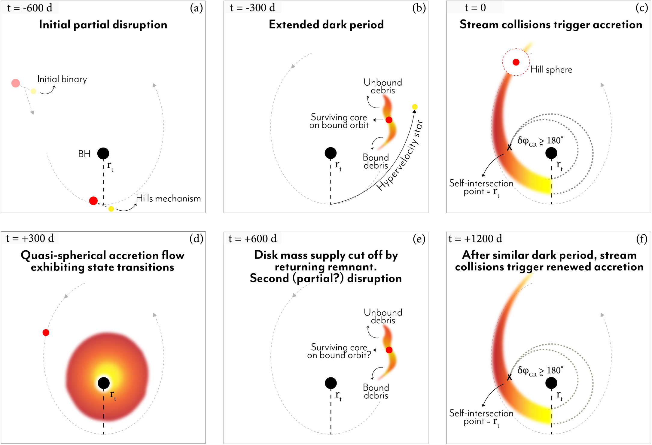
where a⋆ is the binary semimajor axis, and M⋆ is the mass of the primary. A schematic of the different phases of the repeated partial disruption scenario and the timescales involved is shown in Figure 4.

Figure 4. Multipanel schematic indicating the various phases in the evolution of AT 2018fyk. Time is indicated in the top left corner. The various components (SMBH, star, accretion flow) are not to scale. Following panel (f), future observations will show whether the returning core was fully disrupted or if a third dimming and rebrightening cycle occurs.
Download figure:
Standard image High-resolution imageWith a host galaxy velocity dispersion of σ = 158 km s−1, the maximum separation that a binary can have and still survive in the galactic nucleus is a⋆ ≲ GM⋆/(4σ2) ≃ 0.01 au (e.g., Hills 1975; Gould 1991; Quinlan 1996; Yu 2002). With a⋆ = 0.01 au, M⋆ = 1 M⊙, and M = 107.7 M⊙, Equation (1) gives Torb ≃ 2.5 yr. A dynamical exchange can therefore produce a star on an orbit about the SMBH with a period as short as ∼a few years. For separations ≲0.01 au, the tidal disruption radius of the binary is comparable to the tidal disruption radius of the star (increased by stellar rotation and relativistic effects; Gafton et al. 2015; Golightly et al. 2019; Gafton & Rosswog 2019), and a partial TDE will occur (Figures 4(a) and (b)). The tight required separation of the initial binary provides constraints on the maximum size of the stars, in this case, ≲2 R⊙. Such systems would require either two low-mass stars or a main sequence–compact object binary; the latter (with the main-sequence star captured) is favored in order to reproduce the overall energetics and timescales of the TDE, as we now discuss (see Section 4 for additional motivation for this type of binary).
Upon being partially disrupted, the material returns to the SMBH on a timescale that is approximately (Lacy et al. 1982; Rees 1988)

and has a peak magnitude

though these are generally longer and lower, respectively, for partial disruptions (e.g., Guillochon & Ramirez-Ruiz 2013; Miles et al. 2020; Nixon et al. 2021; see also Section 4 below). The proportionality coefficient in Equation (3) matches simulations that yield a peak accretion rate equal to Eddington for M = 107 M⊙, M⋆ = 1 M⊙, and a radiative efficiency η = 0.1 (Wu et al. 2018). Setting M = 107.7 M⊙ and taking solar-like values gives Tacc ≃ 0.8 yr and Lacc ≃ 6.7 × 1044 erg s−1 (Figure 4(b)). Partial TDEs typically rise, peak, and decay as ∝ t−9/4 (Coughlin & Nixon 2019; Miles et al. 2020; Nixon et al. 2021), but for a star on a bound orbit, the fallback rate plummets as the star returns to pericenter (Liu et al. 2022). The reason for this sharp decline in the fallback rate is that the stellar core has a Hill sphere—an approximately spherical region within which the star's gravitational field dominates over that of the SMBH—near which the stream density is much smaller than that of the bulk of the stream (Figure 4(e)). This feature of the fallback rate can physically explain the rapid shutoff displayed in Figure 1 at ∼600 days.
While it likely does not inhibit the formation of a disk, nodal precession—assuming the SMBH has a modest spin—is probably important for its subsequent evolution; over many orbits of the material in the innermost regions of the disk, nodal and apsidal precession, coupled to the (likely) large misalignment angle between the spin axis of the SMBH and the angular momentum of the gas, will cause fluid annuli to precess independently instead of conforming to a smooth, warped disk (Nixon et al. 2012; Liska et al. 2021). The orbit of the returning star also precesses and leads to a time-dependent feeding angle of the flow; thus, the gas is likely morphologically complex and, we suggest, closer to spherically symmetric than in the form of a traditional disk (see also Patra et al. 2022). If we assume that the returning debris stream is cylindrical with a cross-sectional radius of ∼R⊙ and length  (Cufari et al. 2022b), then taking a⋆ = 0.01 au, M = 107.7
M⊙, and with 0.05 M⋆ contained in the stream (see Section 4),
(Cufari et al. 2022b), then taking a⋆ = 0.01 au, M = 107.7
M⊙, and with 0.05 M⋆ contained in the stream (see Section 4),

Taking v = 0.1c as the speed of the material as it shocks (recall that the pericenter is highly relativistic), the shocked-gas pressure is

The fluid is radiation pressure–dominated with a temperature

Equation (6) represents the self-intersection temperature near the horizon. The gas expands roughly adiabatically from the self-intersection point (e.g., Jiang et al. 2016), which reduces the temperature and density. At early times, the gas will be optically thick, the photosphere at large radii, and the peak emission at temperatures below Equation (6). However, as time advances, the fallback rate declines, the density drops due to the continued expansion of the gas, and the flow becomes more optically thin to reveal the hot, inner regions, thus providing a plausible interpretation of the late-time dominance of the X-ray emission.
4. Implications and Predictions
From Wevers et al. (2019) and the additional data obtained since then, the total amount of energy radiated is equivalent to ≈9 × 1051 erg. This energy could be up to a factor of ∼5 smaller 14 if the majority of the energy is not radiated at UV/optical wavelengths, as we have assumed in calculating the bolometric luminosity (and thus the total radiated energy; see Figure 2). If we adopt a radiative efficiency of η = 0.1, the radiated energy amounts to ≈0.05 M⊙ of accreted mass. In normal TDEs (i.e., where the center of mass is on a parabolic orbit), approximately half of the stellar mass is accreted, and this implies that the star lost at most ∼0.1 M⊙ during the tidal encounter. We note that for typical binaries, the ratio of the binding energy of the binary to that of its stellar constituents is very small (on the order of the ratio of the stellar radius to the binary separation); hence, the approximation that only half of the material is accreted is usually warranted. Here, however, the binary must be very tight to reproduce the observed timescales, meaning that the binding energy of the binary is not substantially smaller than that of the star itself, and the "unbound debris" featured in panel (b) of Figure 4 may actually remain bound to the SMBH. If this is the case, we expect the luminosity of the "lesser bound" tail to be significantly lower than that of the more tightly bound tail owing to the longer return time. This material may be of sufficiently low density that it is substantially affected/destroyed by interactions with circumnuclear gas (Bonnerot et al. 2016) and the surviving core as it passes through pericenter a second time. Additional and more detailed investigations are required to constrain the energetics of the unbound/less bound tail.
Because the surviving core is spun up to near its breakup velocity, the tidal radius moves out (Golightly et al. 2019), and it is possible that the star was completely destroyed on its second pericenter passage (Figure 4(f)). If the mass lost from the star is closer to the upper limit of ∼0.1 M⊙ that is inferred from the bolometric luminosity, then it could be that the star was completely destroyed on the second passage, and we would expect the accretion rate to monotonically decline with time. On the other hand, if the bolometric inference significantly overestimates the energy radiated and the mass accreted is closer to ∼0.01 M⊙, it is likely that the star survived and will return to cause another dimming and future flare. Future observations will show if the star survived the second encounter to generate a third flare.
From the eROSITA nondetections between days ∼600 and ∼1200 (although note that the last eROSITA upper limit is only a factor of ∼2–3 below the observed flux level), the fallback time of the material tidally stripped from the star during its second pericenter passage is, from Figure 1, ∼600 days (note that ordinarily, this timescale is virtually impossible to constrain from observations of single TDEs, but it was possible because of fortuitous eROSITA data points). As noted above, the canonical timescale for a TDE between a solar-like star and a 107.7 M⊙ SMBH is Tacc ≃ 0.8 yr ≃ 300 days (see Equation (2)), which is a factor of ∼2 shorter than the observed fallback time.
However, the return time of the most bound debris from a partial TDE can be significantly longer than the canonical value because of the gravitational influence of the surviving core, which is obvious from the fact that the fallback time becomes infinitely long in the limit that no mass is lost. From Figure 4 of Nixon et al. (2021), the return time of the most bound debris from a 1 M⊙ zero-age main-sequence star increases by a factor of ∼ 2–3 in going from β ≃ 2 (where the disruption is full) to β ≃ 1, where the star loses ∼10% of its mass (see Figure 4 of Guillochon & Ramirez-Ruiz 2013 and Figure 5 of Mainetti et al. 2017). Nixon et al. (2021) showed (top panel of their Figure 2) that if the peak in the return time is extended to ∼0.2 yr, implying a return time of ∼0.2 yr × 101.7/2 ∼ 520 days for a 107.7 M⊙ SMBH (comparable to what is observed for AT 2018fyk), we would need β ≲ 0.7 if the star is somewhat evolved and conceivably smaller if the star is near zero-age (Figure 1 of the same paper).
For β ≃ 0.7, Figure 4 of Nixon et al. (2021) predicts a peak luminosity of ∼4 × 1043 erg s−1 (adopting a radiative efficiency η = 0.1) for a 107.7 M⊙ SMBH, which is slightly less than but still in rough agreement with the X-ray luminosity in the top left panel of Figure 1. At this value of β, the amount of mass lost from the star is also predicted from Newtonian simulations to be ≲0.01 M⊙ (e.g., Guillochon & Ramirez-Ruiz 2013; Law-Smith et al. 2020), which is in tension with the estimates from the bolometric luminosity that give a value that is closer to ∼0.1 M⊙. Nonetheless, as we noted, the bolometric luminosity (and thus the total energy radiated) is uncertain for this system, as it is based on a classic accretion disk model where the bulk of the energy is emitted at wavelengths for which we have no data, and the picture outlined here and shown in Figure 4 is clearly quite distinct from a standard disk; the total energy radiated could thus be a factor of ∼5 smaller than the value used to infer the estimate of 0.05 M⊙ accreted (see the discussion at the beginning of this section). Furthermore, general relativistic simulations indicate that more mass is lost from the star for the same β as compared to Newtonian estimates; for example, Figure 3 of Gafton et al. (2015) shows that a β = 0.7 encounter between a solar-like 5/3 polytrope and a 4 × 10⁷ M⊙ SMBH—for which the pericenter distance is ∼5.8 GM/c2—strips ∼70% of the stellar mass, while a 106 M⊙ SMBH removes only ∼25% for the same β. Figures 8–12 of Gafton & Rosswog (2019) show, nonetheless, that the timescales of the TDE remain similar. For our case, in which a Sun-like star is disrupted by a 107.7 M⊙ SMBH, the tidal radius is rt ≃ 3.5GM/c2 and thus highly relativistic. Hence, even for β ≲ 0.7, we would expect a larger fraction of the mass to be lost than would be predicted in the Newtonian limit. Thus, while more detailed modeling is required to more accurately constrain the properties of, e.g., the disrupted star, we find that the overall duration and energetics of the flare are consistent with the partial disruption of a near-solar star. On the other hand, increasing the mass and size of the star would increase the timescale, luminosity, and accreted mass and thus reduce these tensions, but the small separation of the binary restricts the size of the star to ≲1–2 R⊙ to avoid a common envelope phase (see also the last paragraph of this section).
Assuming that the first detection was approximately coincident with the time of the initial outburst, which is consistent with the lack of optical variability (e.g., from the pre-peak ASAS-SN light curve), we infer that the orbital period of the star is ∼1200 days, or ∼3.3 yr (i.e., the star's first pericenter passage was at day ∼−600 relative to discovery). We therefore predict that—if the star was not destroyed on its second pericenter passage—the source will abruptly decline in luminosity again around day 1800 (2023 August) before flaring for a third time (presuming the star is not destroyed on its third pericenter passage) around 15 day ∼2400 (2025 March).
Finally, if the orbital period of the captured star is ≈1200 days, then Equation (1) with M⋆ = 1 M⊙ and M/M⋆ = 107.7 suggests that the separation of the initial binary—which was ripped apart to yield the captured star—had a separation of ∼0.012 au. As noted above, the M–σ relationship with a black hole mass of 107.7
M⊙ implies that binaries must have a separation of less than ∼0.01 au to survive; hence, this binary separation is consistent with the high velocity dispersion in the nucleus of the galaxy. The distributions of observed binaries that are near solar are roughly uniform in semimajor axis or, for higher-mass stars, in  (Opik's law) and thus peaked toward small separations (Offner et al. 2022). Since the hardening rate is roughly constant once the binary has reached a hardened separation (Quinlan 1996), from a probabilistic standpoint, we would also expect those with the widest (but hardened) initial separations to survive long enough to be fed into the galactic nucleus and tidally destroyed.
From the timescales and energetics arguments above (see the discussion around Equations (2) and (3)), the captured star that is repeatedly partially disrupted likely must be near solar in terms of its mass and size. With a separation a ≲ 0.01 au ∼ 2 R⊙, the companion object—which was ejected during the separation of the binary (see Figures 4(a) and (b))—is therefore likely required to be a compact object to avoid being in a common envelope phase (as also argued in Cufari et al. 2022b in the context of the event ASASSN-14ko). If the companion was a white dwarf, which is most likely from a statistical standpoint, then the small binary separation appears consistent with the substantial population of detached white dwarf–main-sequence binaries with semimajor axes ∼1 R⊙ (likely as a consequence of a previous common envelope phase; e.g., Willems & Kolb 2004; Parsons et al. 2015; Mu et al. 2021; Hernandez et al. 2021; Zheng et al. 2022). Thus, in addition to being required from a survivability standpoint and to reproduce the orbital period of the captured star, the small separation of the binary is consistent if the companion is a white dwarf.
5. Summary and Conclusions
After ∼600 days of quiescence, the TDE AT 2018fyk showed an anomalous rebrightening in both the UV and X-ray bands to luminosities to within a factor 10 of their peak values, a behavior that is unprecedented in observations of TDEs. The model we propose to explain this behavior is that the initial flare was caused by the partial disruption of a star that was part of a binary system. The partially disrupted star was captured onto a relatively tight orbit through the destruction of the binary (i.e., Hills capture), thus generating a repeating, partial TDE (as well as a high-velocity star flung out from the system) and the late-time flare. This model is not only consistent with the observations but also predicts that (1) the fallback time of the tidally stripped debris is ∼600 days (a timescale that is, we note, ordinarily very hard to constrain from observations of full TDEs), (2) the orbital time of the captured star is ∼1200 days, and (3) the source should once again dim at day ∼1800 (when the core is expected to return again) and brighten a third time at day ∼2400 if the star was not completely destroyed on its second pericenter passage; on the other hand, if it was completely destroyed, we would expect—as it is then an ordinary TDE—a roughly power-law decay in its luminosity (although, if the star is on a bound orbit, it may exhibit a double-peaked light curve, depending on the eccentricity; Cufari et al. 2022a).
We briefly remark that qualitatively similar behavior, including a late-time rebrightening in the background X-ray emission to ∼60% of its peak magnitude around day ∼3600 postdiscovery, has recently been observed in a source exhibiting quasiperiodic X-ray eruptions (QPEs; Miniutti et al. 2022). To explain their properties, QPEs have also been hypothesized to be the result of repeated tidal stripping, particularly of white dwarfs by low-mass SMBHs (e.g., Arcodia et al. 2021; King 2020; Miniutti et al. 2022). Their host galaxies share several peculiar properties with those of TDEs, including low-mass black holes and a preference for poststarburst galaxies (Wevers et al. 2022).
We finish by highlighting the importance of X-ray and UV monitoring observations of TDEs at late times. Almost all TDEs identified so far lack long-term (yearslong) follow-up. This leaves significant uncertainty as to whether similar behavior has occurred in other TDEs. For example, van Velzen et al. (2019) reported a deep UV upper limit for the source SDSS-TDE1, but no other meaningful constraints exist in the ∼6 yr prior to that observation. Similarly, the majority of TDEs have either no or extremely sparse UV and X-ray constraints at late times. One exception to this is the recently reported observations of AT 2021ehb, a TDE that similarly shows accretion state transitions at late times (Yao et al. 2022), although a partial TDE scenario is not necessary to explain that behavior. Long-term monitoring observations of TDEs—particularly for those with high-mass SMBHs, where partial TDEs are very likely—may provide more evidence for partial TDEs in the future. Indeed, highly periodic flaring may be among the most unambiguous signatures of a partial TDE in general.
We thank the anonymous referee for thoughtful comments and suggestions that helped to improve the manuscript. We thank the XMM, Swift, and NICER PIs (Norbert Schartel, Bradley Cenko, and Keith Gendreau) and their operations teams for approving and promptly scheduling the requested observations. We warmly thank M.I. Saladino for help in creating Figure 4. E.R.C. thanks Chris Nixon for useful discussions and acknowledges support from the National Science Foundation through grant AST-2006684 and the Oakridge Associated Universities through a Ralph E. Powe Junior Faculty Enhancement Award. Raw optical/UV/X-ray observations are available in the NASA/Swift archive (http://heasarc.nasa.gov/docs/swift/archive; target names: AT 2018fyk, ASASSN-18UL) and XMM-Newton Science Archive (http://nxsa.esac.esa.int; ObsID: 0911790601, 0911791601); NICER data are publicly available through the HEASARC: https://heasarc.gsfc.nasa.gov/cgi-bin/W3Browse/w3browse.pl. Based on observations collected at the European Southern Observatory under ESO programs 0103.D-0440(B) and 0106.21SS.
This work is based on data from eROSITA, the soft X-ray instrument on board SRG, a joint Russian–German science mission supported by the Russian Space Agency (Roskosmos), in the interests of the Russian Academy of Sciences represented by its Space Research Institute (IKI), and the Deutsches Zentrum für Luft- und Raumfahrt (DLR). The SRG spacecraft was built by Lavochkin Association (NPOL) and its subcontractors and is operated by NPOL with support from the Max Planck Institute for Extraterrestrial Physics (MPE).
The development and construction of the eROSITA X-ray instrument was led by MPE, with contributions from the Dr. Karl Remeis Observatory Bamberg & ECAP (FAU Erlangen-Nuernberg), the University of Hamburg Observatory, the Leibniz Institute for Astrophysics Potsdam (AIP), and the Institute for Astronomy and Astrophysics of the University of Tübingen, with the support of DLR and the Max Planck Society. The Argelander Institute for Astronomy of the University of Bonn and the Ludwig Maximilians Universität Munich also participated in the science preparation for eROSITA.
The eROSITA data shown here were processed using the eSASS software system developed by the German eROSITA consortium.
Appendix A: Supplementary Material
A.1. Observations and Data Reduction
A.2. Swift XRT and UVOT
We reduce the UV/Optical Telescope (UVOT; Roming et al. 2005) data using the uvotsource task, extracting fluxes from the standard 5'' aperture. We subsequently correct for Galactic extinction assuming E(B – V) = 0.01 (Schlafly & Finkbeiner 2011) and subtract the host galaxy contribution as determined from SED fitting in Wevers et al. (2021). The emission in the UV bands has brightened by a factor of ∼10, although in the optical, this is much less pronounced, with the brightness in the B and V filters remaining consistent with the inferred host galaxy brightness. We therefore do not include these filters in our analysis. The UV light curves can be found in the online supplementary material. The Swift/XRT light curve and late-time stacked spectrum were extracted using the online XRT tool. 16
A.3. XMM-Newton
A 29 ks observation was approved by the XMM-Newton director and executed on 2022 May 20/21 (ObsID: 0911790601). The optical monitor used the UVW1 filter, taking five deep images, as well as a small window centered on the galaxy nucleus with data in time-tag (fast) mode. The EPIC instruments (PN, MOS1, and MOS2) were operated in full-frame mode with the thin1 filter. The observation was split into two blocks, one of 20 ks and one of 9 ks. The latter was unfortunately lost due to telemetry problems. An additional 10 ks observation was therefore scheduled on 2022 June 9, with an identical instrument setup (ObsID: 0911791401).
We start by reprocessing the data using the emproc and epproc tasks in XMM-SAS v1.3. Good time intervals (GTIs) are identified by excluding periods of background flaring in the 10–12 keV band. This leaves approximately 9.2 ks of exposure for the observation with ID 0911790601, while 3.5 ks remains for ID 0911791401. We therefore only use the data of ObsID 0911790601 for our analysis. The background is estimated from a source-free region with radius 50'' on the same detector, while the source signal is extracted from a region with radius 33''. After applying standard data filters, we extract spectra and light curves in the 0.3–10 keV energy range. Light curves are further corrected for instrumental effects using the epiclccorr task.
A.4. NICER/XTI
NICER is a nonimaging detector with 52 coaligned concentrators that focus X-rays onto silicon drift detectors at their respective foci. It has a field of view of 3 1 in radius and a nominal bandpass of 0.2–12 keV. But, depending on the source brightness and background, the usable bandpass can vary. NICER's large effective area of >1700 cm2 at 1 keV enabled by its 52 focal plane modules (FPMs) and ability to steer rapidly to any part of the sky and monitor sources for extended periods of months and years makes it an excellent telescope for tracking long-term transients like TDEs.
Following the Swift/XRT detection of AT 2018fyk, NICER started a high-cadence monitoring program as part of an approved guest observer program (ID: 5070; PI: Pasham). NICER data are organized in the form of ObsIDs that represent a collection of short exposures or GTIs varying from 100 s to up to 2000 s over the time span of a day. While NICER monitoring of AT 2018fyk continues at the time of writing of this paper, we include all data taken prior to 2022 August 22.
We started our NICER data analysis by downloading the raw, unfiltered data from the HEASARC public archive. These were reduced using the standard reduction procedures of running nicerl2 followed by nimaketime. All of the filter parameters except for overonly_range, underonly_range, and overonly_expr were set to the default values as recommended by the data analysis guide: https://heasarc.gsfc.nasa.gov/lheasoft/ftools/headas/nimaketime.html. The reason for not screening on undershoots and overshoots is to ensure we are not throwing away good data in the name of strict default screening values. Instead, we screen each GTI based on the net, i.e., background-subtracted, 0–0.2, 13–15, and 4–12 keV count rates as recommended by Remillard et al. (2022). After a background spectrum is estimated using the 3c50 model, if the absolute value of the net count rate in 0–0.2 keV is more than 2 cps, the absolute value of the net rate in 13–15 keV is more than 0.05 cps, or the absolute value of the net 4–12 keV is more than 0.5 cps, we mark that GTI as bad and omit it from further analysis (see Pasham et al. 2021 for more details).
To improve statistics, we also extracted 18 time-resolved spectra by combining multiple GTIs. Spectra were binned with the optimal binning scheme of Kaastra & Bleeker (2016). To do this, we used the ftool ftgrouppha with an additional requirement to have a minimum of 20 counts per spectral bin. Object AT 2018fyk was above the background in the 0.3–0.7 keV bandpass. Because of this limited bandpass, we fit each spectrum with a simple power law plus a Gaussian model (tbabs*zashift(pow) + Gaussian in XSPEC) and inferred the best-fit power-law index and absorption-corrected 0.3–10 keV luminosities. The Gaussian component was used to model out the variable-strength background oxygen line at 0.54 keV from the Earth's atmosphere. A summary of the spectral modeling is shown in Table A2.
Table A2. Summary of Time-resolved X-Ray Energy Spectral Modeling of AT 2018fyk
| Best-fit Parameters from Fitting Time-resolved 0.3–0.7 keV NICER X-Ray Spectra | |||||||||
|---|---|---|---|---|---|---|---|---|---|
| Start | End | Exposure | FPMs | Phase | Γ | log(Integ. Lum.) | log(Obs. Lum.) | Count Rate | Gaussian |
| (MJD) | (MJD) | (ks) | (0.3–10 keV) | (0.3–10.0 keV) | (0.3–10.0 keV) | Norm. | |||
| 59,682.51 | 59,689.0 | 0.87 | 51 | L1 |

|

|

| 0.0055 ± 0.0024 |

|
| 59,693.7 | 59,698.27 | 2.6 | 43 | L2 |

|

|

| 0.0166 ± 0.0012 |

|
| 59,698.27 | 59,703.0 | 5.45 | 47 | L3 |

|

|

| 0.0093 ± 0.0006 |

|
| 59,703.0 | 59,708.0 | 8.68 | 46 | L4 |

|

|

| 0.0095 ± 0.0003 |

|
| 59,708.0 | 59,718.0 | 9.1 | 49 | L5 |

|

|

| 0.0073 ± 0.0003 |

|
| 59,718.0 | 59,723.0 | 3.46 | 51 | L6 |

|

|

| 0.0057 ± 0.0007 |

|
| 59,723.0 | 59,728.0 | 5.12 | 50 | L7 |

|

|

| 0.0055 ± 0.0005 |

|
| 59,728.0 | 59,733.0 | 3.69 | 50 | L8 |

|

|

| 0.0052 ± 0.0007 |

|
| 59,733.0 | 59,738.0 | 3.63 | 52 | L9 |

|

|

| 0.0056 ± 0.0007 |

|
| 59,738.0 | 59,743.0 | 3.23 | 52 | L10 |

|

|

| 0.0055 ± 0.0008 |

|
| 59,743.0 | 59,748.0 | 4.76 | 52 | L11 |

|

|

| 0.0041 ± 0.0005 |

|
| 59,748.0 | 59,758.0 | 10.3 | 52 | L12 |

|

|

| 0.0038 ± 0.0002 |

|
| 59,758.0 | 59,768.0 | 2.53 | 51 | L13 |

|

|

| 0.0056 ± 0.0009 |

|
| 59,768.0 | 59,778.0 | 4.14 | 51 | L14 |

|

|

| 0.0048 ± 0.0006 |

|
| 59,778.0 | 59,783.0 | 6.03 | 52 | L15 |

|

|

| 0.0055 ± 0.0004 |

|
| 59,783.0 | 59,788.0 | 5.06 | 52 | L16 |

|

|

| 0.006 ± 0.0005 |

|
| 59,788.0 | 59,798.0 | 7.05 | 52 | L17 |

|

|

| 0.0066 ± 0.0004 |

|
| 59,798.0 | 59,820.0 | 8.22 | 52 | L18 |

|

|

| 0.0052 ± 0.0003 |

|
Note. Here 0.3–0.7 keV NICER spectra are fit with the tbabs*zashift(clumin*pow) + Gaussian model using XSPEC (Arnaud 1996). Start and End represent the start and end times (in units of MJD) of the interval used to extract a combined NICER spectrum. Exposure is the accumulated exposure time during this time interval. The FPMs are the total number of active detectors minus the "hot" detectors. Phase is the name used to identify the epoch, Γ is the photon index of the power-law component, log(Integ. Lum.) is the logarithm of the integrated absorption-corrected power-law luminosity in 0.3–10 keV in units of erg s−1, and log(Obs. Lum.) is the logarithm of the observed, extrapolated 0.3–10.0 keV luminosity in units of erg s−1. Count rate is the background-subtracted NICER count rate in 0.3–0.7 keV in units of counts per second per 50 FPMs. All error bars represent 1σ uncertainties. The total best-fit χ2/degrees of freedom over all spectra is 76.5/65.
Download table as: ASCIITypeset image
A.5. SRG/eROSITA
Coinciding with the quiescent phase following the first major optical outburst, AT 2018 fyk was observed every 6 months by SRG/eROSITA (Sunyaev et al. 2021; Predehl et al. 2021) during its first four all-sky surveys (denoted eRASS1, 2, 3, and 4, respectively; a log of observations is presented in Table A3). No X-ray point source was detected by the eROSITA Science Analysis Software pipeline (eSASS; Brunner et al. 2022) within  of the optical position of AT 2018 fyk during these scans. Using the eSASS task SRCTOOL (v211214), source counts were extracted from a circular aperture of radius
  centered on the optical position of AT 2018 fyk, while background counts were extracted from a source-free annulus with inner and outer radii of
  and
and  , respectively. The inferred 3σ upper limits on the 0.3–2 keV count rates in each eRASS scan were (0.067, 0.063, 0.16, 0.14) counts s−1 on MJD (58,981.348, 59,165.818, 59,348.557, and 59,532.943), respectively. Assuming the best-fitting spectral model from the XMM observation in Table A1, these rates correspond to upper limits on the 0.3–2 keV observed fluxes of (1.4, 1.2, 3.4, and 3.1) × 10−13 erg s−1 cm−2, respectively. A 0.3–2 keV 3σ upper limit on the source count rate from the stack of eRASS1–4 observations is 0.032 counts s−1 (observed 0.3–2 keV flux of 6.5 × 10⁻¹⁴ erg s−1 cm−2). Based on the spectral model derived from the XMM-Newton observation, we calculate a correction factor of 1.46 for the conversion from the 0.3–2 to 0.3–10 keV band. We report the 0.3–10 keV band values throughout the manuscript for consistency with data from other observatories.
Table A3. Log of SRG/eROSITA Observations of AT 2018 fyk During Its All-sky Survey
| eRASS | Exposure | MJD Start | MJD Stop | Phase | Rate | FX,obs |
|---|---|---|---|---|---|---|
| (s) | (days) | (counts s−1) | (10−13 erg s−1 cm−2) | |||
| eRASS1 | 206 | 58,980.848 | 58,981.848 | 612.148 | <0.067 | <1.4 |
| eRASS2 | 172 | 59,165.401 | 59,166.235 | 796.618 | <0.063 | <1.2 |
| eRASS3 | 124 | 59,348.223 | 59,348.890 | 979.357 | <0.162 | <3.4 |
| eRASS4 | 179 | 59,532.610 | 59,533.277 | 1163.743 | <0.138 | <3.1 |
Note. The MJD start and stop columns refer to the times of the first and last observation of AT 2018 fyk within a given eRASS, with the phase then being measured based on the midpoint of these relative to MJD = 58,369.2. The rate and FX,obs columns are the observed source count rates and observed fluxes computed in the 0.3–2 keV band (not corrected for Galactic absorption).
Download table as: ASCIITypeset image
A.6. MUSE
On 2019 June 10 (MJD 58,644), AT 2018fyk was observed by MUSE (Bacon et al. 2010) as part of the All-weather MUse Supernova Integral field Nearby Galaxies (AMUSING) survey, ESO ID: 0103.D-0440(B). At this epoch, the transient was already quiescent at optical wavelengths, and the host galaxy emission completely dominated the data. The data cube was analyzed as part of the AMUSING++ Nearby Galaxy Compilation (López-Cobá et al. 2020). However, the authors did not include it in the final sample of the paper due to the lack of strong emission lines, which were the main subject of their study. Nevertheless, we obtained the final products of their stellar population and emission line fitting analyses (López-Cobá, private communication).
A detailed description is presented in López-Cobá et al. (2020). In summary, the following procedure was adopted. First, the raw data cubes were reduced with REFLEX (Freudling et al. 2013) using version 0.18.5 of the MUSE pipeline. Next, the emission lines and stellar population content were analyzed using the PIPE3D pipeline (Sánchez et al. 2016a), a fitting routine adapted to analyze IFS data using the package FIT3D (Sánchez et al. 2016b). The procedure starts by performing a spatial binning on the continuum (V band) to increase the signal-to-noise ratio in each spectrum of the data cube. The stellar population model was derived by performing stellar population synthesis; the PIPE3D implementation adopts the GSD156 stellar library, which comprises 39 ages and four metallicities, extensively described in Cid Fernandes et al. (2013). Then, a model of the stellar continuum in each spaxel was recovered by rescaling the model within each spatial bin to the continuum flux intensity in the corresponding spaxel. The best model for the continuum was then subtracted to create a pure gas data cube. A set of 30 emission lines within the MUSE wavelength range were fit spaxel by spaxel for the pure gas cube by performing a nonparametric method based on a moment analysis. The data products of the pipeline are a set of bidimensional maps of the considered parameters with their corresponding errors.
In Figure A1, we show the sample of these maps with the main parameters of interest for this study. The galaxy shows a centrally concentrated structure, like most TDE hosts (Hammerstein et al. 2022); a very old stellar population (mean age ≥109.7 yr); a lack of dust (AV* ≤ 0.05 in all spaxels); and very faint emission lines (mean EW Hα < 1 Å), without any apparent increase toward the central spaxels.

Figure A1. MUSE stellar continuum-subtracted emission line maps.
Download figure:
Standard image High-resolution imageA.7. X-shooter
The host galaxy was observed in long-slit mode with the X-shooter instrument on the Very Large Telescope Unit Telescope 3 on 2020 October 16 (MJD 59,138.08). Slit widths of 1 0, 09, and 09 were deployed for the UVB, VIS, and NIR arms, respectively, for a total exposure time of 1300 s. The average seeing of 07 during the observations results in a seeing-limited spectral resolution of R = 7700 (UVB), 12,700 (VIS), and 8000 (NIR), equivalent to an FWHM spectral resolution of 40 (at 4000 Å) and 25 (at Hα) km s−1. The data were taken in on-slit nodding mode, but to increase the signal-to-noise ratio of the UVB and VIS arms, we reduce these data using the X-shooter pipeline with recipes designed for stare mode observations.
We modeled the stellar continuum of the X-shooter spectrum with a wavelength range of 4000–7000 Å in the rest frame using the penalized pixel fitting (Cappellari 2017) routine. We masked some emission and absorption lines that are usually significant in galaxy spectra, since they may affect the best fits of stellar continuum models, e.g., Hδ, Hγ, Hβ, Hα, N ii 4640, He ii 4686, [O iii] 4959, 5007, He i 5875, [O i] 6300, [N ii] 6548, 6584, and [S ii] 6717, 6731. We used MILES single stellar population (SSP) models (Vazdekis et al. 2010) as the stellar templates and adopted the SSP model spectra. Given that the initial resolution of the X-shooter spectrum is R ∼ 10,000, much higher than that of the MILES spectra (R ∼ 2000), we convolved the X-shooter spectrum to reduce its resolution to R ∼ 2000. Except for the stellar template, a polynomial with degree = 4 was added to avoid mismatches between galaxy spectra and stellar templates. The residuals were obtained after subtracting the best-fit stellar continuum model. Residual flux errors are the same as the original flux errors. Line ratios and EWs were measured on the residual spectra, and uncertainties were determined by taking into account the flux uncertainties. The resampled galaxy spectrum overlaid with the fit and residuals after template subtraction are shown in Figure A2.

Figure A2. The X-shooter spectrum (black), resampled to the native resolution of the MILES stellar template library. The best-fit template is shown in blue, and the residuals (offset by +0.4 for clarity) are shown in orange. Weak narrow emission lines appear after template subtraction. Balmer lines are indicated by vertical solid lines, and other emission lines measured for the diagnostic diagrams are marked by dotted lines. The discontinuity between 5300 and 5400 Å is due to the stitching of the two arms.
Download figure:
Standard image High-resolution image
Footnotes
- 10
Note that the assumption of hot blackbody emission down to 0.03 μm cannot be verified because the extreme ultraviolet is not observationally accessible (see also Figure 2).
- 11
There are hints of variability similar to that observed in the earlier hard state, but due to the larger error bars, firm conclusions are not possible.
- 12
A retired galaxy has neither current star formation nor an active nucleus; instead, its post–asymptotic giant branch stellar population can ionize the diffuse gas, producing EW Hα up to 3 Å, with line ratios that can occupy the LINER section of the BPT; see, e.g., Stasińska et al. (2008) and Cid Fernandes et al. (2010, 2011) for detailed discussions.
- 13
The covering factor fc is defined as the ratio between the dust IR luminosity and the optical luminosity. It measures the fraction of the produced radiation that is absorbed by dust, hence the amount of dust in the nuclear region.
- 14
The integral under the observed SED yields a luminosity lower by a factor of ∼5 compared to that of the total model SED (which yields the bolometric luminosity). The true value will be somewhere in between these two estimates.
- 15
The rapid rotation of the surviving core shortens the fallback time of the debris (Golightly et al. 2019), but we expect ∼2400 days to roughly correspond with when the source will brighten a third time.
- 16