


Abstract
We report the first unambiguous detection of an axial merger shock in the early-stage merging cluster Abell 98 using deep (227 ks) Chandra observations. The shock is about 420 kpc south from the northern subcluster of Abell 98, in between the northern and central subclusters, with a Mach number of  ≈ 2.3 ± 0.3. Our discovery of the axial merger shock front unveils a critical epoch in the formation of a massive galaxy cluster, when two subclusters are caught in the early phase of the merging process. We find that the electron temperature in the postshock region favors the instant collisionless model, where electrons are strongly heated at the shock front, by interactions with the magnetic field. We also report on the detection of an intercluster gas filament, with a temperature of kT = 1.07 ± 0.29 keV, along the merger axis of Abell 98. The measured properties of the gas in the filament are consistent with previous observations and numerical simulations of the hottest, densest parts of the warm–hot intergalactic medium (WHIM), where WHIM filaments interface with the virialization regions of galaxy clusters.
Export citation and abstract BibTeX RIS
1. Introduction
Clusters of galaxies are primarily assembled and grow via accretion, gravitational infall, and mergers of smaller substructures and groups. In such merging events, a significant fraction of kinetic energy dissipates (on a Gyr timescale) in the intracluster medium (ICM) via shocks and turbulence (Markevitch et al. 1999). Such shocks are the major heating sources for the X-ray emitting ICM plasma (Markevitch & Vikhlinin 2007). Shock fronts provide an essential observational tool in probing the physics of transport processes in the ICM, including electron–ion equilibration and thermal conduction, magnetic fields, and turbulence (e.g., Markevitch 2006; Markevitch & Vikhlinin 2007; Botteon et al. 2016, 2018).
Despite the intrinsic interest and significance of merger shocks, X-ray observations of merger shocks with a sharp density edge and an unambiguous jump in temperature are relatively rare. Currently, only a handful of merger shock fronts have been identified by Chandra, such as 1E 0657-56 (Markevitch et al. 2002), A520 (Markevitch et al. 2005), A2146 (Russell et al. 2010, 2012), A2744 (Owers et al. 2011), A754 (Macario et al. 2011), A2034 (Owers et al. 2014), and A665 (Dasadia et al. 2016).
Cosmic filaments are thought to connect the large-scale structures of our universe (e.g., Dolag et al. 2006; Werner et al. 2008; Alvarez et al. 2018; Reiprich et al. 2021). Several independent searches for baryonic mass have confirmed discrepancies in baryonic content between the high- and low-redshift universe (e.g., Fukugita et al. 1998; Fukugita & Peebles 2004), with fewer baryons being detected in the local universe. They concluded that a significant fraction of these missing baryons may be "hidden" in the WHIM, in cosmic filaments that connect clusters and groups. The WHIM has a temperature in the 105–107 K (or, kT ∼ 0.01–1 keV) regime, and relatively low surface brightness (e.g., Davé et al. 1999; Cen & Ostriker 1999; Davé et al. 2001; Smith et al. 2011).
Abell 98 (hereafter A98) is a richness class III early-stage merger with three subclusters: central (A98S; z ≈ 0.1063), northern (A98N; z ≈ 0.1042), and southern (A98SS; z ≈ 0.1218). The northern and southern subclusters are at projected distances of ∼1.1 Mpc and 1.4 Mpc from the central subcluster, respectively (e.g., Abell et al. 1989; Burns et al. 1994; Jones & Forman 1999; Paterno-Mahler et al. 2014). The central subcluster is undergoing a separate late-stage merger, with two distinct X-ray cores. Previous observations using Chandra and showed that A98N is a cool core cluster with a marginal detection of a warm gas arc, consistent with the presence of a leading bow shock, but that the exposure time was insufficient to confirm this feature (Paterno-Mahler et al. 2014).
To investigate further, we analyzed deep (∼227 ks) Chandra observations of A98N and A98S. In this Letter, we report on the detection of an intercluster filament connecting A98N and A98S, and of a leading bow shock in the region of the filament, associated with the early-stage merger between A98N and A98S. We adopted a cosmology of H0 = 70 km s−1 Mpc−1, ΩΛ = 0.7, and Ωm = 0.3, which gives a scale of 1'' = 1.913 kpc at the redshift z = 0.1042 of A98. Unless otherwise stated, all reported error bars are at 90% confidence level.
2. Data Analysis
A98 was observed twice with Chandra for a total exposure time of ∼227 ks. The observation logs are listed in Table 1. We discuss the detailed data reduction processes in Appendix A.
2.1. Imaging Analysis
The image showing the both A98N and A98S in the 0.5–2 keV energy band are shown in Figure 1. We derived a Gaussian gradient magnitude (GGM) filtered image of A98, zooming in the northern subcluster, as shown in Figure 2. The GGM-filtered image provides a powerful tool to reveal substructures and any associated sharp features in the cluster core, as well as at larger cluster radii (Walker et al. 2016). The intensity of the GGM images indicates the slope of the local surface brightness gradient, with steeper gradients showing up as brighter regions. The GGM image we present here is filtered on a length scale of 32 pixels. Each pixel is 0.492'' wide. We observe a rapid change in the magnitude of the surface brightness gradient at ∼400 kpc to the south of the A98N center, as seen in Figure 2.
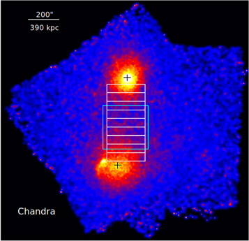
Figure 1. Chandra exposure-corrected and background-subtracted image of A98 in the 0.5–2 keV energy band. White and cyan regions are used for the analysis of the filament emission. Centers of A98N and A98S are marked in black.
Download figure:
Standard image High-resolution image
Figure 2. Top left: similar to Figure 1, but zoomed in to A98N and smoothed with a σ = 2'' Gaussian. Green regions used for spectral analysis. Top right: GGM image of A98N with a σ = 16'' Gaussian kernel. White dashed curve shows the southern shock front. Middle left: surface brightness profile of A98N in the south direction with 1σ error bars. Inset figure shows the 3D density profile. Middle right: projected temperature; bottom left: 3D density; bottom right: pressure profiles of A98N in the south direction.
Download figure:
Standard image High-resolution imageGGM images often show artifacts from the filtering process, particularly in low surface brightness regions. Therefore, we next test for the presence of the edge feature indicated in Figure 2 by extracting a surface brightness profile across the edge. Figure 2 shows the resulting radial surface brightness profile as a function of distance from the A98N core in the 0.5–2 keV energy band. We observe an edge in the X-ray surface brightness profile at about 420 kpc (0:46:23.14, +20:33:46.32) from the A98N core. The distance of the edge from the A98N core is consistent with the edge observed in the GGM image, which suggests the abrupt change in the gradient corresponds to the surface brightness edge.
The shape of the extracted surface brightness profile across the edge is consistent with what is expected from a projection of a 3D density discontinuity (Markevitch et al. 2000). To quantify the surface brightness edge, we fit the surface brightness profile by projecting a 3D discontinuous double power-law model along the line of sight, defined as
where ne
(r) is the 3D electron density at a radius r, redge is the radius of the putative edge, jump is the density jump factor, and α1 and α2 are the slopes before and after the edge, respectively. A constant term was also added to the model to account for any residual background, after blank-sky subtraction. The best-fit value of this term was consistent with zero, suggesting we successfully eliminated sky and particle background. We project the estimated emission measure profile onto the sky plane and fit the observed surface brightness profile by using least-squares fitting technique with α1, α2, redge, and jump as free parameters. Figure 2 shows the best-fit model and the 3D density profile (inset). The best-fit power-law indices across the edge are α1 = 0.76 ± 0.01 and α2 = 0.83 ± 0.02, respectively (χ2/dof = 57/21). The density jumps, across the edge, by a factor of ρ2/ρ1 = 2.5 ± 0.3, where suffixes 2 and 1 represent the regions inside and outside of the front. Assuming that the edge is a shock front, this density jump corresponds to a Mach number of  = 2.3 ± 0.3, estimated from the Rankine–Hugoniot jump condition, defined as
where r = ρ2/ρ1 and for a monoatomic gas γ = 5/3. The edge radius, obtained from the fit, is 420 ± 25 kpc. We estimated the uncertainties by allowing all the other model parameters to vary freely. The best-fit edge radius is consistent with the distance of the GGM peak from the A98N center.
2.2. Spectral Analysis
To measure the temperature across the surface brightness edge, the southern sector was divided into seven regions, as shown in Figure 2. Each region contains a minimum of 2300 background-subtracted counts. We set this lower limit to guarantee adequate counts to measure the temperature uncertainty within 25% in the faint region at a 90% confidence level. For each region, we extracted spectra from individual observations and fitted them simultaneously. The spectra were grouped to contain a minimum of 20 counts per spectral channel. The blank-sky-background spectra were subtracted from the source spectra before fitting (Dasadia et al. 2016). We fitted the spectra from each region to an absorbed single-temperature thermal emission model, PHABS(APEC) (Smith et al. 2001). The redshift was fixed to z = 0.1042, and the absorption was fixed to the Galactic value of NH = 3.06 × 1020 cm−2 (Kalberla et al. 2005). The spectral fitting was performed using XSPEC in the 0.6–7 keV energy band, and the best-fit parameters were obtained by reducing C-statistics. We fixed the metallicity to an average value of 0.4 Z⊙ since it was poorly constrained if left free (Russell et al. 2010). We adopted the solar abundance table of Asplund et al. (2009).
Figure 2 shows the best-fit projected temperatures. The projected temperature increases steadily from the A98N core up to ∼200 kpc, then jumps to a peak of ∼ keV at ∼420 kpc, which then plummets to
  keV beyond the surface brightness edge. Across the edge, the temperature decreases by a factor of ∼2.3 ± 0.6, confirming the outer edge as a shock front. We estimated the electron pressure by combining the temperature and electron density, as shown in Figure 2. As expected, we found a significant decrease in pressure by a factor of ∼7 ± 2 at the shock front. The observed temperature drop corresponds to a Mach number of
  = 2.2 ± 0.4, consistent with the Mach number derived from the density and pressure jump. Mach numbers from both methods are consistent with each other, bolstering the shock detection. We estimated a preshock sound speed of cs
∼ 848 ± 80 km s−1, which gives a shock speed of vshock =
= 2.2 ± 0.4, consistent with the Mach number derived from the density and pressure jump. Mach numbers from both methods are consistent with each other, bolstering the shock detection. We estimated a preshock sound speed of cs
∼ 848 ± 80 km s−1, which gives a shock speed of vshock =  ≈ 1900 ± 180 km s−1.
3. Detection of Filament Emission
Early-stage, major mergers between two roughly equal mass subclusters are expected to typically have their merger axis aligned with the filaments of the cosmic web (see Alvarez et al. 2018 for further discussion). To search for faint X-ray emission associated with the filament between A98N and A98S, we extracted a surface brightness profile from nine box regions across the bridge between A98N and A98S in the 0.5–2 keV energy band (see Figure 1). Figure 3 shows the surface brightness profile of the bridge. This surface brightness profile includes the emission from the extended ICM of both subclusters, and from the filament. To account for only the extended ICM emission from both subclusters, we extracted surface brightness profiles from similar regions placed in the opposite directions of the filament, using Suzaku observations of A98 (Alvarez et al. 2022), assuming in each that the contribution from the neighboring subcluster is negligible. We used Suzaku observations because the existing Chandra observations do not cover the part of the sky needed for such analysis. These two diffuse surface brightness profiles are then subtracted from the surface brightness profile of the bridge, yielding the surface brightness profile of the filament. We use WebPIMMS 9 to convert Suzaku and Chandra count rates to physical units (erg cm−2 s−1 arcsec−2) in the 0.5–2 keV energy band. We assumed a thermal APEC model with absorption fixed to NH = 3.06 × 1020 cm−2, abundance Z = 0.2Z⊙, and temperature kT = 2.6 keV (as discussed later in the current Section).
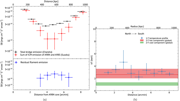
Figure 3. Left: black shows the surface brightness profile across the bridge measured using Chandra. Red indicates the sum of the surface brightness profiles of the diffuse, extended emission extracted from the Suzaku observations. Blue represents the residual filament emission. Right: projected temperature profile across the bridge, measured with a 1-T model. Red and green shaded regions indicate the hot component and cool component temperatures, respectively, measured with a 2-T model.
Download figure:
Standard image High-resolution imageFigure 3 shows the resulting surface brightness profile of the filament in the 0.5–2 keV energy band. We detected excess X-ray surface brightness in the region of the bridge with a ∼3.2σ significance level. Similar excess emission along the bridge with somewhat lower significance (∼2.2σ) was also found by Alvarez et al. (2022) using only Suzaku data. Being very nearby to both subcluster cores, where emission is dominated by the respective subcluster, we could not detect any significant filament emission from the first two and last two regions. This excess X-ray emission suggests the presence of a filament along the bridge connecting A98N and A98S.
To measure the temperature across the bridge region, we adopted similar regions used for the surface brightness profile of the bridge. The spectra were then fitted to a single-temperature APEC model (1-T), keeping the metallicity fixed to 0.2 Z⊙. Figure 3 shows the projected temperature profile. The temperatures across the bridge are consistent within their ∼2.7σ (90%) uncertainty, except for third region where we detected a shock. We next measured the global properties of the bridge using a 0.6 Mpc × 0.7 Mpc box region (632 kpc from the A98N and 505 kpc from the A98S; shown with cyan in Figure 1). Using a single-temperature emission model for the bridge region, we obtained a temperature of  keV and an abundance of
  Z⊙. Our measured temperature of the bridge is consistent with the temperatures obtained by Paterno-Mahler et al. (2014) using XMM-Newton and relatively short exposure Chandra observations. We next estimated the electron density of the bridge using

where N is APEC normalization, DA
is the angular diameter distance, r and lobs are the radius and the projected length of the filament, respectively. We obtained an electron density of ne
= 4.2 × 10⁻⁴ cm−3, assuming the filament is in the plane of the sky (i = 90°) and has cylindrical symmetry, since for i ≪ 90° we would not expect to detect a clear leading merger shock edge. Our measured temperature and electron density are higher than the expected temperature (≲1 keV) and electron density (∼10−4 cm−3) for the WHIM (e.g., Bregman 2007; Werner et al. 2008; Eckert et al. 2015; Alvarez et al. 2018; Hincks et al. 2022).
The surface brightness profiles seen in Figure 3 show that the emission from the filament itself is much fainter than the diffuse, extended cluster emission. A low-density gas emission is expected together with the ICM emission at the bridge region. We, therefore, adopted a two-temperature emission model for the bridge and obtained a temperature of kThot = 2.60 keV for the hotter component and kTcool = 1.07 ± 0.29 keV for the cooler component. The higher temperature gas is probably mostly the overlapping extended ICM of the subclusters seen in projection. The two-temperature model was a marginal improvement over the one-temperature model with an F-test probability of 0.08. The emission measure of the cooler component corresponds to an electron density of ne
= 1.30
keV for the hotter component and kTcool = 1.07 ± 0.29 keV for the cooler component. The higher temperature gas is probably mostly the overlapping extended ICM of the subclusters seen in projection. The two-temperature model was a marginal improvement over the one-temperature model with an F-test probability of 0.08. The emission measure of the cooler component corresponds to an electron density of ne
= 1.30 × 10⁻⁴ cm−3, assuming the filament is in the plane of the sky. From the temperature and electron density of the cooler component, we obtain an entropy of ∼416 keV cm2. Our measured temperature, density, and entropy of the cooler component are consistent with what one expects for the hot, dense part of the WHIM (e.g., Eckert et al. 2015; Bulbul et al. 2016; Alvarez et al. 2018; Reiprich et al. 2021). Suzaku observations also show similar emission to the north of A98N, beyond the virial radius, in the region of the putative large-scale cosmic filament (Alvarez et al. 2022). We also check for any systematic uncertainties in measuring the filament temperature, abundance, and density by varying the scaling parameter of blank-sky background spectra by ±5%. We find no significant changes.
4. Discussion and Conclusion
4.1. Nature of the Shock Front
Our deep Chandra observations reveal that the overall system is complex, with A98S dominated by a later-stage merger ongoing along the east–west direction (A. Sarkar et al. 2022, in preparation). Previously, Paterno-Mahler et al. (2014) argued that the surface brightness excess along the southern direction of A98N is more likely a shock with a Mach number,  ≳ 1.3. With the new data, we found that the temperature increases by a factor of ∼2.3 (from 2.7 to 6.4 keV) across the surface brightness edge, confirming it is a shock front propagating along the merger axis (N/S direction). This is the first unambiguous detection of axial merger shock in an early-stage merger (i.e., pre-core-passage), as opposed to the late-stage merger (i.e., post-core-passage), where several previous observations found axial shocks (e.g., Russell et al. 2010, 2012; Dasadia et al. 2016).
Axial shock detection in an early-stage merging cluster is a long-standing missing piece of the puzzle of cluster formation. Previous Chandra observations of the premerger system, 1E 2216/1E 2215, detected an equatorial shock (Gu et al. 2019). Equatorial shocks are driven by the adiabatically expanding overlap region between the outskirts of the merging subclusters. They propagate along the equatorial plane, perpendicular to the merger axis. This is in contrast to axial shocks, which are driven by, and ahead of, the infalling subclusters. Gu et al. (2019) did not detect any axial shock in 1E 2216/1E 2215. There are conflicting findings from simulations on which merger shock should form first. Recent hydrodynamical simulations of binary cluster mergers by Zhang et al. (2021) showed the formation of axial merger shocks in the early stages of the merging process. In contrast, simulations by Ha et al. (2018) indicated that equatorial shock forms long before the axial shock.
To date, it is unclear what is driving the apparent discrepancy between the formation of equatorial and axial shocks, although the parameters of the merger (e.g., mass ratio, total mass, impact parameter) likely play a role. Our Chandra observation of the shock front in A98 is the "first" unambiguous axial shock detection in an early-stage merging system, prior to core passage. We detect no equatorial shocks, but it is possible that they are present and the current observations are not deep enough to detect them. With this discovery, we caught two subclusters in a crucial epoch of the merging process, which will reveal any missing link to the shock formation process in premerger systems and provide a yardstick for future simulations.
4.2. Electron–Ion Equilibrium
The electron heating mechanism behind a shock front is still up for debate. The collisional equilibrium model predicts that a shock front propagating through a collisional plasma heats the heavier ions dissipatively. Electrons are then compressed adiabatically, and subsequently come to thermal equilibrium with the ions via Coulomb collisions after a timescale defined in Equation (B1) (Spitzer 1962; Sarazin 1988; Ettori & Fabian 1998; Markevitch & Vikhlinin 2007). By contrast, the instant equilibrium model predicts that electrons are strongly heated at the shock front, and their temperature rapidly rises to the postshock gas temperature, similar to the ions (Markevitch 2006; Russell et al. 2012). The electron and ion temperature jumps at the shock front are determined by the Rankine–Hugonoit jump conditions. Markevitch (2006) showed that the observed temperature profile across the shock front of the Bullet cluster supports the instant equilibrium model. Russell et al. (2012) found that the temperature profile across one shock front of A2146 supports the collisional model while another shock supports the instant model. However, in all cases the measurement errors prevented a conclusive determination. Later, Russell et al. (2022) with deeper Chandra observations found both shocks in A2146 favor the collisional model.
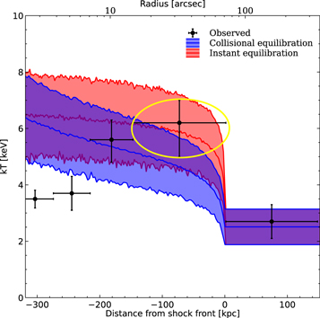
Here, we compare the observed temperature profile across the shock front of A98 with the predicted temperature profiles from collisional and instant equilibrium models. We estimate the model electron temperatures and project them along the line of sight, as described in Appendix B. The resulting temperature profiles are shown in Figure 4. The observed postshock electron temperature appears to be higher than the temperature predicted by the collisional equilibrium model and favors the instant equilibrium model, although we cannot rule out the collisional equilibration model due to the large uncertainty in the postshock electron temperature.
Figure 4. Comparison of the temperature profile across the shock front with the predicted electron temperature profiles based on the instant collisionless model (red) and the Coulomb collisional model (blue). Yellow ellipse indicates the relevant postshock electron temperature for comparing with two models.
Download figure:
Standard image High-resolution image
4.3. Filament Emission
We detected 3.2σ excess X-ray emission along the bridge connecting two subclusters (A98N and A98S), also detected by Alvarez et al. (2022) (with lower significance) using Suzaku. Our measured surface brightness of the cooler component ranges between (0.9–2.8) × 10−15 erg cm−2 s−1 arcmin−2 in the 0.5–2 keV energy band, which is equivalent to (1.2–3.6) ×10−15 erg cm−2 s−1 arcmin−2 in the 0.2–10 keV energy band. Using high-resolution cosmological simulations, Dolag et al. (2006) predicted that the X-ray surface brightness of the WHIM filaments should be ∼10−16 erg cm−2 s−1 arcmin−2 with a zero metallicity in the 0.2–10 keV energy band. However, an increased metallicity could induce more line emission, increasing the surface brightness of the filament. A similar conclusion was drawn by Werner et al. (2008) while explaining their observed surface brightness of the WHIM filament, higher than that of cosmological simulation. Our measured surface brightness of the filament is consistent with the surface brightness of the WHIM filament obtained for A222/223 and A1750 (Bulbul et al. 2016).
Using a 2-T plasma emission model, we measured the temperature of the cooler component of the filament, kTcool = 1.07 ± 0.29 keV. The 2-T model was a marginal improvement over the 1-T model with an F-test probability of 0.08. Similar filament temperatures were measured for A2744 (0.86–1.72 keV; Eckert et al. 2015), A222/223 (0.66–1.16 keV; Werner et al. 2008), and A1750 (Bulbul et al. 2016). We obtained a best-fit filament electron density of ne
= 1.30 × 10⁻⁴ cm−3, assuming the filament is in the sky plane. If the filament has an inclination angle (i) with the line of sight, the electron density will be lower by a factor of (
 )−1/2. Previous studies also found similar electron densities for the hot, dense part of the WHIM in several other galaxy clusters, e.g., 0.88 × 10⁻⁴ cm−3 for A399/401 (Hincks et al. 2022), 1.08 × 10⁻⁴ cm−3 for A3391/3395 (Alvarez et al. 2018), and 10−4 cm−3 for A2744 and A222/223 (Werner et al. 2008; Eckert et al. 2015). We estimated a baryon overdensity of ρ/〈ρ〉 ∼ 240 associated with the gas in the filament, which is consistent with the expected overdensity for a WHIM filament (Bregman 2007). Assuming a cylindrical geometry for the filament, we estimated the associated gas mass to be Mgas = 3.8
 × 1011
M⊙.
× 1011
M⊙.
Our measured temperature and average density of the cooler component are remarkably consistent with what one expects for the hot, dense part of the WHIM, suggesting that this gas corresponds to the hottest, densest parts of the WHIM. X-ray observations of the emission from WHIM filaments are relatively rare because they have a lower surface brightness than the ICM. They offer crucial observational evidence of hierarchical structure formation. Using numerical simulations, Davé et al. (2001) predicted that the gas in a WHIM filament has a temperatures in the range 105.5–106.5 K. A similar conclusion was drawn by Lim et al. (2020) using the kinetic S–Z effect in groups of galaxies. Since our detected filament lies in the overlapping ICM of both subclusters, the gas may have been heated by the shock and adiabatic compression.
We are grateful to the anonymous referee for insightful comments that greatly helped to improve the Letter. This work is based on observations obtained with Chandra observatory, a NASA mission and Suzaku, a joint JAXA and NASA mission. A.S. and S.R. are supported by the grant from NASA's Chandra X-ray Observatory, grant number GO9-20112X.
Appendix A: Data Reduction Processes
A98 was observed twice with Chandra ACIS-I in VFAINT mode, in 2009 September for 37 ks split into two observations and later in 2018 September–2019 February for 190 ks divided into eight observations. The combined exposure time is ∼227 ks (detailed observation logs are listed in Table 1). The Chandra data reduction was performed using CIAO version 4.12 and CALDB version 4.9.4 provided by the Chandra X-ray Center (CXC). We have followed a standard data analysis thread. 10
Table 1. Chandra Observation Log
| Obs ID | Obs Date | Exp. Time | PI |
|---|---|---|---|
| (ks) | |||
| 11876 | 2009 Sep 17 | 19.2 | S. Murray |
| 11877 | 2009 Sep 17 | 17.9 | S. Murray |
| 21534 | 2018 Sep 28 | 29.5 | S. Randall |
| 21535 | 2019 Feb 19 | 24.7 | S. Randall |
| 21856 | 2018 Sep 26 | 30.5 | S. Randall |
| 21857 | 2018 Sep 30 | 30.6 | S. Randall |
| 21880 | 2018 Oct 09 | 9.9 | S. Randall |
| 21893 | 2018 Nov 11 | 17.9 | S. Randall |
| 21894 | 2018 Nov 14 | 17.8 | S. Randall |
| 21895 | 2018 Nov 14 | 28.6 | S. Randall |
Download table as: ASCIITypeset image
All level 1 event files were reprocessed using the chandra_repro task, employing the latest gain and charge transfer inefficiency corrections, and standard grade filtering. VFAINT mode was applied to improve the background screening. The light curves were extracted and filtered using the lc_clean script to identify and remove periods affected by flares. The filtered exposure times are listed in Table 1. We used the reproject_obs task to reproject all observations to a common tangent position and combine them. The exposure maps in the 0.5–2.0 keV energy bands were created using the flux_obs script by providing a weight spectrum. The weight spectrum was generated using the make_instmap_weights task with an absorbed APEC plasma emission model and a plasma temperature of 3 keV. To remove low signal-to-noise areas near chip edges and chip gaps, we set the pixel value to zero for those pixels with an exposure of less than 15% of the combined exposure time.
Point sources were identified using wavdetect with a range of wavelet radii between 1 and 16 pixels to maximize the number of detected point sources. We set the detection threshold to ∼10−6, for which we expect ≲1 spurious source detection per CCD. We used blank-sky observations provided by the CXC to model the non-X-ray background and emission from the foreground structures (e.g., Galactic Halo and Local Hot Bubble) along the observed direction. The blank-sky background was generated using the blanksky task and then reprojected to match the coordinates of the observations. The resulting blank-sky background was normalized so that the hard-band (9.5–12 keV) count rate matched the observations.
Appendix B: Electron Heating Mechanism
When a shock front propagates through a plasma, it heats the ions dissipatively in a layer that has a width of few ion–ion collisional mean free paths. On the other hand, having very high thermal velocity compared to the shock, the electron temperature does not jump by the same high factor as the ion temperature. The electrons are compressed adiabatically at first in merger shocks and subsequently equilibrate with the ions via Coulomb scattering after a timescale (Spitzer 1962; Sarazin 1988) given by
where Te and ne are the electron temperature and density, respectively.
Alternatively, the instant collisionless shock model predicts that the electrons and ions reach thermal equilibrium on a timescale much shorter than teq after passing the shock front, where the postshock electron temperature is determined by the preshock electron temperature and the Rankine–Hugonoit jump conditions (Markevitch & Vikhlinin 2007). We use the best-fit density profile shown in Figure 2 to project this model electron temperature along the line of sight analytically (Russell et al. 2012).
In the collisional equilibration model, the electron temperature rises at the shock front through adiabatic compression,
where ρ1 and ρ2 are the gas density in the preshock and postshock regions, and γ = 5/3. Electron and ion temperatures then subsequently equilibrate via Coulomb collision at a rate given by

where Ti is the ion temperature. Since the total kinetic energy density is conserved, the local mean gas temperature, Tgas, is constant with time, where Tgas is given by

where ni is the ion density.
We integrate Equation (B3) by using Equations (B1) and (B4) to obtain the model electron temperature analytically. Finally, we project the model electron temperature profile along the line of sight (Ettori & Fabian 1998) by
where  (r) is the emissivity at physical radius r and b is the distance from the shock front.
The emissivity-weighted electron temperature should be close to what one observes with a perfect instrument with a flat energy response across the relevant energy range. Since this is not the case, we convolve the instant and collisional model electron temperatures with the response of the telescope to predict what we expect to measure (Russell et al. 2012). We first estimate the emissivity-weighted electron temperature using the above models and corresponding emission measure using the best-fit density discontinuity model (Equation (3)) in a small volume dV. We then sum the emission measures with similar temperatures for each annulus using a temperature binning of 0.1 keV. We simulate spectra in XSPEC using a multitemperature absorbed apec model. We fix the temperature of each component with the median temperature of each bin and calculate the normalization based on the summed emission measure in that temperature bin. We also fix the abundance to 0.4 Z⊙, NH to galactic value, and redshift to 0.1043. To estimate the expected projected temperature in this annulus, we finally fit this simulated spectra with a single-temperature absorbed apec model with abundance, NH, and redshift fixed as above.
We adopt the Monte Carlo technique with 1000 realizations to measure uncertainty in model electron temperatures. Assuming a Gaussian distribution of the preshock temperature, which is the largest source of uncertainty, we repeated the model and projected temperature calculations 1000 times with a new value of preshock temperature each time. The resulting instant and collisional model temperature profiles with 1σ uncertainty are shown in Figure 4.
Footnotes
- 9
- 10