


Abstract
The structure of the electron diffusion region (EDR) is essential for determining how fast the magnetic energy converts to plasma energy during magnetic reconnection. Conventional knowledge of the diffusion region assumes that the EDR is a single layer embedded within the ion diffusion region (IDR). This paper reports the first observation of two EDRs that stack in parallel within an IDR by the Magnetospheric Multiscale mission. The oblique tearing modes can result in these stacked EDRs. Intense electron flow shear in the vicinity of two EDRs induced electron Kelvin–Helmholtz vortices, which subsequently generated kinetic-scale magnetic peak and holes, which may effectively trap electrons. Our analyses show that both the oblique tearing instability and electron Kelvin–Helmholtz instability are important in three-dimensional reconnection since they can control the electron dynamics and structure of the diffusion region through cross-scale coupling.
Export citation and abstract BibTeX RIS

Original content from this work may be used under the terms of the Creative Commons Attribution 4.0 licence. Any further distribution of this work must maintain attribution to the author(s) and the title of the work, journal citation and DOI.
1. Introduction
Magnetic reconnection is a fundamental magnetic energy release process in space, astrophysical, and laboratory plasma systems. It is a multiscale process that couples plasma systems from the magnetohydrodynamic (MHD) scale down to the particle's kinetic scale. In collisionless reconnection, a commonly recognized model is the Hall model that can account for the fast reconnection rate widely observed in space. An essential ingredient of this model is the two-dimensional (2D) nested diffusion region, which includes an ion-scale diffusion region (IDR) and an embedded electron-scale diffusion region (EDR), where magnetic field lines break and reconnect to cause large-scale energy release (Deng & Matsumoto 2001; Øieroset et al. 2001; Eastwood et al. 2010; Burch et al.2016b; Torbert et al. 2018). However, this is a rough schematic of the diffusion region in a laminar current sheet. The diffusion region may develop three-dimensional (3D) structures that induce large-amplitude fluctuations and substantially affect the energy release process through reconnection.
Recent 3D kinetic simulations show that kinetic-scale instabilities significantly affect the electron dynamics, which alters the structure of the diffusion region, setting it apart from the conventional description. The lower hybrid drift instability developed along the X-line substantially disturbs the X-line and leads to a turbulent diffusion region (Roytershteyn et al. 2012; Price et al. 2016). The electron shear instability can drive the filamentation of reconnecting current sheets, providing anomalous viscosity for reconnection (Che et al. 2011). Liu et al. (2013) demonstrate that multiple EDRs may be stacked within a broader ion-scale diffusion region due to the oblique tearing modes at different electron resonance layers. In situ observations are urgently required to resolve fine structures of the diffusion region.
Here we report the first evidence for two stacked EDRs and electron flow vortices generated by the cross-scale coupling of the oblique tearing instability and electron Kelvin–Helmholtz (K-H) instability within a single reconnection layer. The reconnection occurs in the magnetosheath downstream of the quasi-perpendicular bow shock and was observed by the Magnetospheric Multiscale (MMS) mission (Burch et al. 2016a). Data used in this study are from the following instruments of the MMS: The Fluxgate Magnetometer (Russell et al. 2016), the Fast Plasma Investigation (Pollock et al. 2016), and the Electric Double Probe (Ergun et al. 2016; Lindqvist et al. 2016). The solar wind magnetic field is from the OMNI data set.
2. Event Overview
Figure 1 presents the OMNI data and MMS measurements during 06:15:00–07:10:00 UT on 2015 October 5, when MMS was around (7.9, 5.2, −0.1) RE in the Geocentric Solar Ecliptic (GSE) coordinates. The absence of an electron population above 1 keV (Figure 1(e)) indicates that MMS was in the magnetosheath proper during this interval. Using the bow shock model (Chao et al. 2002) based on the OMNI data, we find that MMS was downstream of the quasi-perpendicular bow shock.

Figure 1. Overview of the OMNI data and MMS2 measurements during 06:15:00–07:10:00 UT. (a) Three components of the interplanetary magnetic fields approximately shifted to the bow shock. (b)–(e) MMS2 observations in the magnetosheath: (b) three components of the magnetic field, (c) total magnetic field, and (d) ion and (e) electron differential energy fluxes. The GSE coordinate is employed.
Download figure:
Standard image High-resolution imageFigure 1(b) shows that the magnetic field Bz reverses several times during this interval, while Bx and By are mostly negative and positive, respectively. The directions of the magnetic fields in the magnetosheath (Figure 1(b)) correlate well with those in the solar wind (Figure 1(a)). The structures characterized by Bz reversals in the solar wind and magnetosheath are discontinuities or current sheets originating from the solar wind. The time delay of these current sheets observed by MMS relative to OMNI data is about 5–10 minutes as indicated by the black arrows in Figures 1(a) and (b). In addition, intense magnetic field fluctuations with amplitude above 50% of the background magnetic field (Figure 1(c)) were observed during the entire interval when MMS was in the magnetosheath. Thus, the current sheets were immersed within a turbulent plasma. In the following, we focus on one of these current sheets, which is highlighted by the magenta-shaded regions in Figure 1. Its thickness in the solar wind was estimated as 55,800 km ∼ 547 di (1 di ∼ 102 km is the ion inertial length based on the average plasma density 5 cm−3) by using the solar wind speed ∼ 465 km s−1.
Figures 2(a)–(g) present the MMS observations around this current sheet after it crossed the bow shock. The sharp reversal of Bz
(Figure 2(a)) corresponds to an intense current with a peak density of 600 nA m−2 at around 06:36:20.00 UT (Figure 2(g)). The magnetic field strength ∣B∣ (Figure 2(b)) fluctuates quasi-monochromatically (with respect to the average magnetic field) on both sides of the current sheet. The quasi-monochromatic fluctuation of Ne
(Figure 2(c)) is anti-correlated to the fluctuation of ∣B∣, indicating a mirror-type mode. Figure 2(e) shows that the perpendicular ion temperature Ti⊥ (blue curve) was greater than the parallel ion temperature Ti∥ (red curve) during this interval. This significant ion temperature anisotropy satisfies the threshold of the ion-mirror instability (Figure 2(f)),  , where
  is the perpendicular ion plasma β. All these features imply that these quasi-monochromatic fluctuations were ion-mirror-mode structures (Ahmadi et al. 2017; Zhang et al. 2018). The wavelength of the mirror-mode structures was about (2500–6250) km ∼ (58–145) di
(1 di
∼ 43 km given the plasma density 28 cm−3), which is estimated by assuming mirror waves being convected with the background ion bulk flow.
is the perpendicular ion plasma β. All these features imply that these quasi-monochromatic fluctuations were ion-mirror-mode structures (Ahmadi et al. 2017; Zhang et al. 2018). The wavelength of the mirror-mode structures was about (2500–6250) km ∼ (58–145) di
(1 di
∼ 43 km given the plasma density 28 cm−3), which is estimated by assuming mirror waves being convected with the background ion bulk flow.
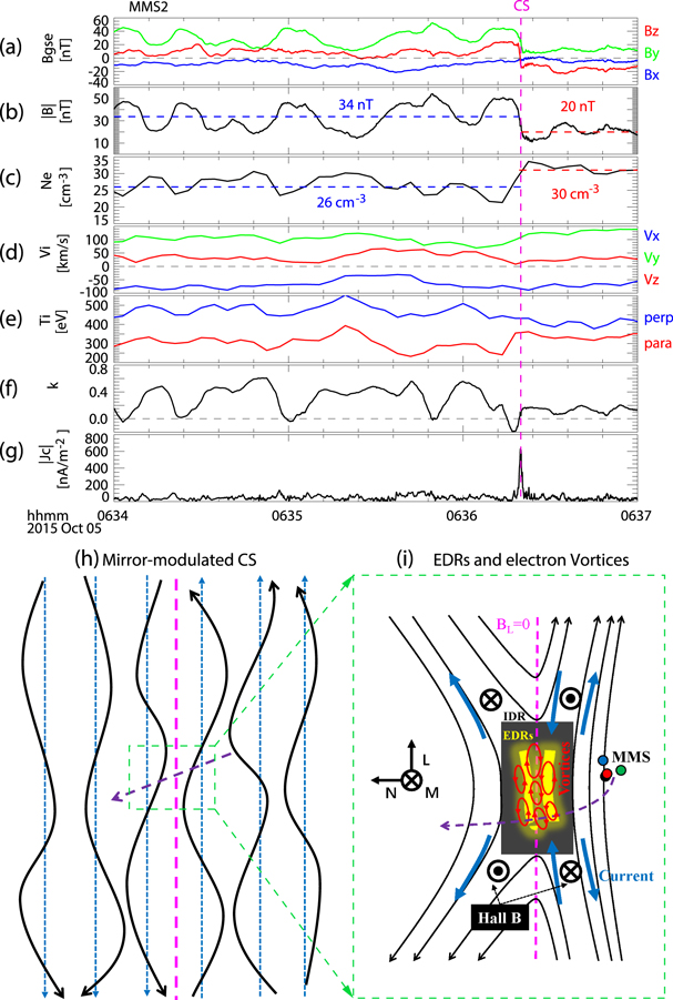
Figure 2. MMS2 observations between 06:34:00 and 06:37:00 UT. (a) Three components of the magnetic field, (b) total magnetic field, (c) electron density, (d) ion bulk velocities, (e) ion temperatures, (f) the parameter  , which is critical to the ion-mirror instability, (g) current density estimated by the curlometer method (the quality factor for the MMS tetrahedron is 0.77), Jc
= ∇ × B. (h) Sketch of the mirror-modulated reconnecting current sheet; the blue dashed lines are the unperturbed magnetic field, the magenta dashed line indicates the center of the current sheet, and the black solid lines represent the mirror-modulated magnetic field. (j) Sketch of two EDRs and electron flow vortices (red rings) within the IDR.
, which is critical to the ion-mirror instability, (g) current density estimated by the curlometer method (the quality factor for the MMS tetrahedron is 0.77), Jc
= ∇ × B. (h) Sketch of the mirror-modulated reconnecting current sheet; the blue dashed lines are the unperturbed magnetic field, the magenta dashed line indicates the center of the current sheet, and the black solid lines represent the mirror-modulated magnetic field. (j) Sketch of two EDRs and electron flow vortices (red rings) within the IDR.
Download figure:
Standard image High-resolution imageWe take the average plasma and magnetic field properties (marked by the dashed lines in Figures 2(b) and (c)) on the two sides of the current sheet as the initial undisturbed properties (before the excitation of the mirror-mode waves) on both sides of the current sheet (Table A1 in the Appendix), respectively. Then, we can investigate the effects of these ion-mirror-mode waves on the current sheet. The estimated initial shear angle of the magnetic field is about 68° and the difference of the ion plasma β,  , across the current sheet is Δβi
≈ 8.6. In comparison, the shear angle is about 73° and Δβi
≈ 32.2 when MMS was crossing the current sheet (Table A1). These indicate that the mirror-mode waves did not substantially change the magnetic field shear angle, but significantly increased the asymmetry of ion plasma β between two sides of the current sheet, which will increase the drift velocity of the X-line due to the diamagnetic drift (Swisdak et al., 2003). Furthermore, the growth of the ion-mirror-mode waves likely perturbed the magnetic field in the direction normal to the current sheet (Figure 2(h)).
, across the current sheet is Δβi
≈ 8.6. In comparison, the shear angle is about 73° and Δβi
≈ 32.2 when MMS was crossing the current sheet (Table A1). These indicate that the mirror-mode waves did not substantially change the magnetic field shear angle, but significantly increased the asymmetry of ion plasma β between two sides of the current sheet, which will increase the drift velocity of the X-line due to the diamagnetic drift (Swisdak et al., 2003). Furthermore, the growth of the ion-mirror-mode waves likely perturbed the magnetic field in the direction normal to the current sheet (Figure 2(h)).
3. Stacked EDRs and Oblique Tearing Modes
Figure 3 details the reconnection signatures of this current sheet in the local boundary normal (LMN) coordinate system. N points sunward along with the current sheet normal direction, L is the maximum variation direction that points in the direction of the reconnecting magnetic field component, and M completes a right-handed orthogonal coordinate system, i.e., M = N × L . The transformation from GSE to LMN coordinates, which was obtained by the minimum variance analysis (Sonnerup & Scheible 1998) on magnetic fields observed by MMS2 during the current sheet crossing between 06:36:18.660 and 06:36:20.410 UT, is given by L = (0.005, 0.397, 0.918), M = (0.165, −0.905, 0.391), N = (0.986, 0.150, −0.070). BL reverses from positive to negative (Figure 3(a)) and the total magnetic field decreases from 48 to 13 nT associated with the electron density increasing from 20 to 30 cm−3 (Figure 3(b)), suggesting an asymmetric current sheet.
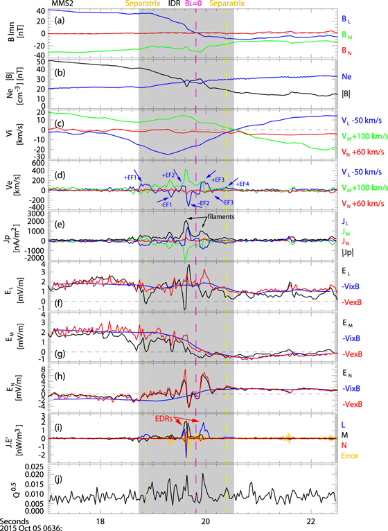
Figure 3. Two EDRs observed in an IDR by MMS2. (a) Three components of the magnetic field; (b) total magnetic field and electron density; (c) ion bulk velocities; (d) electron bulk velocities; (e) current densities calculated from plasma moments, Jp = en(vi − ve ); (f)–(h) three components of the measured electric field (black), −vi × B (blue), −ve × B (red); (i) energy dissipation J · (E + ve × B); (j) electron nongyrotropy Q0.5. The two yellow dashed lines mark the two separatrices.
Download figure:
Standard image High-resolution imageThe current sheet was convected downstream with the ambient flow at a speed of (VL , VM , VN ) ∼(50, −100, −60) km s−1. This ambient flow has been removed from the measured ion and electron bulk velocity (Figures 3(c) and (d)), respectively. The ion bulk velocity viL increases by ∼ 25 km s−1 in the − L direction during the BL reversal interval (Figure 3(c)). It is the reconnection outflow in the − L direction, with a speed about 28% of the asymmetric hybrid Alfvén speed ∼ 90 km s−1 (see Table A2 in the Appendix; Cassak & Shay 2007; Swisdak & Drake 2007; Malakit et al. 2010; Liu et al. 2018a). This implies that the spacecraft may have crossed an IDR where the ion outflow has not fully developed. The above signatures indicate that MMS crossed a reconnecting current sheet on the − L side of an active X-line (Figure 2(i)).
There are four positive electron flows in the L direction (marked by +EF1, +EF2, +EF3, +EF4) observed by all four spacecraft in the current sheet (Figure 3(d), and Figures A1(d), A2(d), and A3(d) in the Appendix). In addition, electron flows −EF1 and −EF2 in the − L direction were observed by all four spacecraft (Figures 3(d), A1(d), A2(d), and A3(d)), while the electron flow in the − L direction −EF3 was observed by MMS2 (Figure 3(d)) and MMS4 (Figure A3(d)). Contrary to the ion flow, these flows along the − L direction are sandwiched by the positive electron flows in the L direction. The structure of these electron flows is more complicated than that in a 2D simulation with a weak/zero guide field (e.g., Swisdak et al. 2018), implying that the 3D effects or guide field is important in this event. JM presents multiple peaks at ∼ 03:36:19.20, 03:36:19.60, and 03:36:19.90 UT (Figure 3(e)), which is different from the bifurcated current sheet in previous studies (e.g., Schindler & Hesse 2008; Wang et al. 2018). Flows +EF1 and +EF4 were located at the two edges of the current sheet, from which the magnetic field BL starts to decrease. The total current ∣J∣ and out-of-plane current JM are close to 0 outside these two edges (Figures 3(e), A1(e), A2(e), and A3(e)). Hence, +EF1 and +EF4 were the two electron inflows at two reconnection separatrices (marked by the yellow dashed lines). In addition, +EF2 and +EF3 are close to the current sheet center where BL = 0, which is different from the electron jets observed at the separatrix region reported by Wang et al. (2017).
Figure 3(h) shows that the
N
component of the ion convective electric field − balances the measured electric field EN
beyond the current sheet but deviates from EN
within the current sheet. In contrast, the
N
component of the electron convective electric field −
balances the measured electric field EN
beyond the current sheet but deviates from EN
within the current sheet. In contrast, the
N
component of the electron convective electric field − balances the EN
during the plotted interval, suggesting that the normal electric field is the Hall electric field. MMS observed a negative–positive–negative variation (after removing the small-scale variations) of the current density JL
(blue curve in Figure 3(e)) during the current sheet crossing. It is consistent with the change of BM
from positive to negative with respect to the negative guide field according to Ampere's law (Figure 3(a)), indicating that the Hall magnetic field was observed by MMS in this current sheet as illustrated in Figure 2(i). The observed Hall electromagnetic fields further imply that MMS detected an IDR (the gray shaded region). The normal speed of the current sheet was estimated to be ∼50 km s−1 using the multi-spacecraft timing method (Schwartz 1998) on the reference point of BL
= 0. This speed agrees with the ambient flow speed in the normal direction. Thus, the thickness of the IDR was estimated as 50 × 2.5 = 125 km ∼ 2.9 di
(1 di
∼ 43 km, given plasma density 28 cm−3 in the magnetosheath). We conclude that an MHD-scale current sheet originating from the solar wind (Figure 1(a)) was compressed to the kinetic scale as it passed through the bow shock (Phan et al. 2007).
balances the EN
during the plotted interval, suggesting that the normal electric field is the Hall electric field. MMS observed a negative–positive–negative variation (after removing the small-scale variations) of the current density JL
(blue curve in Figure 3(e)) during the current sheet crossing. It is consistent with the change of BM
from positive to negative with respect to the negative guide field according to Ampere's law (Figure 3(a)), indicating that the Hall magnetic field was observed by MMS in this current sheet as illustrated in Figure 2(i). The observed Hall electromagnetic fields further imply that MMS detected an IDR (the gray shaded region). The normal speed of the current sheet was estimated to be ∼50 km s−1 using the multi-spacecraft timing method (Schwartz 1998) on the reference point of BL
= 0. This speed agrees with the ambient flow speed in the normal direction. Thus, the thickness of the IDR was estimated as 50 × 2.5 = 125 km ∼ 2.9 di
(1 di
∼ 43 km, given plasma density 28 cm−3 in the magnetosheath). We conclude that an MHD-scale current sheet originating from the solar wind (Figure 1(a)) was compressed to the kinetic scale as it passed through the bow shock (Phan et al. 2007).
There are two intense current filaments on either side of BL = 0, characterized by the two peaks in the total current density ∣Jp ∣ determined from plasma moments (Figure 3(e)). They cannot be seen in the current density estimated by the curlometer method, i.e., Jc = ∇ × B (Figure 2(g)), implying that their spatial scale is smaller than the spacing (∼ 36 km on average) of the spacecraft. The currents of the two filaments were carried by electrons. Electrons decoupled from the magnetic field in these two current filaments characterized by the L and M components of the nonideal electric field, i.e., E + (ve × B) ≠ 0 (Figures 3(f) and (g)), respectively. The large current density and nonideal electric field result in two strong energy dissipation layers that are associated with clear electron nongyrotropy manifested by the two peaks in the parameter Q0.5 (Figure 3(j)) (Swisdak 2016). The peaks of the parameter Q0.5 at the first and second EDR are about 0.02–0.04 in four spacecraft observations, which are 2–4 times the ambient value (∼ 0.01) and are comparable to the Q0.5 values in some of the EDRs reported by Webster et al. (2018). These indicate that these two current filaments are two EDRs (Burch et al. 2016b; Zhou et al. 2017, 2019; Torbert et al. 2018; Zhong et al. 2018, 2020), which were stacked in parallel within a single IDR. Additionally, the nearly monotonic variation of BL as MMS crossed the current sheet further indicates that there are two EDRs, each of which is located on one side of BL = 0, rather than a single deformed EDR (see Figure A4 in the Appendix). The thickness of the first EDR was 5.5 km ∼ 5.5 de ∼ 0.13 di and the second EDR was 10 km ∼ 10 de ∼ 0.23 di . The distance between the two EDRs was 25 km ∼ 25 de ∼ 0.58 di .
Multiple EDRs stacked within one IDR were demonstrated using 3D kinetic simulations (Liu et al. 2013) in the regimes with weak magnetic shear ϕ < 80°. It was shown that this new morphology is caused by oblique tearing modes unstable simultaneously at different electron resonance layers. Based on the magnetic fields on the two sides of the current sheet (the red and blue arrows in Figure 4(i)), the unstable range of tearing instability can be determined (Daughton et al. 2011; Liu et al. 2013, 2018b), as indicated by the gray shaded area in Figure 4(i). Most of the currents observed by MMS (during 06:36:19.00–06:36:21.00 UT) in the L – M plane (color dots in Figure 4(i)) are inside the gray shaded range, suggesting that this is a tearing-dominated current sheet, with the two EDRs corresponding to two different electron resonance layers of the oblique tearing modes. The thickness of the broader current sheet is about 2.9 di , hence the stacked EDRs enable the ion-scale oblique tearing modes during this 3D magnetic reconnection event.
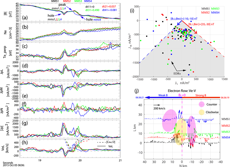
Figure 4. Oblique tearing instability and electron K-H instability in the current sheet. Left column: time-shifted observations of all four spacecraft (see Figure A5 in the Appendix for the original observations). (a) Total magnetic field, (b) electron number density, (c) electron perpendicular temperature, (d)–(f) three components of the current density, (g) total current density, and (h) L component of the electron bulk velocity and the half local electron Alfvén speed. Right column: measurements during 06:36:19.00–06:36:21.00 UT. (i) The current density in the L – M plane JLM (color dots); the magnetic field in the L – M plane BLM (blue and red arrows) on the two sides of the current sheet defines the unstable range of the tearing instability predicted by the theory (marked by the gray shaded area). (j) Electron flow vectors (with uniform background flow, VL = 50 km s−1, VN = −60 km s−1 removed) in the L – N plane. The location of MMS in the N direction is estimated according to the normal velocity of the current sheet (calculated by the timing method), with N = 0 corresponding to the normal position at the time when BL = 0.
Download figure:
Standard image High-resolution image4. Electron Vortices and Electron K-H Instability
We note that both veL
(Figure 3(d)) and JL
(Figure 3(e)) present a bipolar variation at the first EDR, which corresponds to a small dip of ∣B∣ (Figure 3(b)) observed by MMS2. The small dip of ∣B∣ (Figure 4(a)) and JL
bipolar variation (Figure 4(d)) were observed by all four spacecraft at the first EDR (see Figure A5 in the Appendix for the original observations). This dip was associated with a slight enhancement of the electron density (Figure 4(b)) and the electron perpendicular temperature (Figure 4(c)). JN
observed by MMS1 and MMS2 is positive, while it has a bipolar variation in the MMS3 measurement and a negative value in the MMS4 measurement (Figure 4(f)). A magnetic dip consistent with bipolar JL
and JN
was also observed by MMS4 just after the second EDR (Figures 4(d) and (f)), while the bipolar JL
and JN
after the second EDR were not clearly observed by the other spacecraft. These were small-scale electron flow vortices (Zhong et al. 2018, 2019) around the EDRs. Figure 4(j) shows the measurements of electron flow vectors  from all four MMS spacecraft on the
L
–
N
plane. Here the ambient ion flow velocity (VL
= 50 km s−1 and VN
= −60 km s−1) has been removed from the measured electron flows. Two counterclockwise electron flow vortices and one clockwise electron flow vortex were observed within the IDR (Figure 4(j)). The size of these electron flow vortices was larger than 25 km ∼ 25de
in the
L
direction and was about 10 km ∼ 10de
in the
N
direction. Hence, these flow vortices may be elongated in the
L
direction.
from all four MMS spacecraft on the
L
–
N
plane. Here the ambient ion flow velocity (VL
= 50 km s−1 and VN
= −60 km s−1) has been removed from the measured electron flows. Two counterclockwise electron flow vortices and one clockwise electron flow vortex were observed within the IDR (Figure 4(j)). The size of these electron flow vortices was larger than 25 km ∼ 25de
in the
L
direction and was about 10 km ∼ 10de
in the
N
direction. Hence, these flow vortices may be elongated in the
L
direction.
Previous studies suggested that the electron flow vortices can be generated by the electron K-H instability (Fermo et al. 2012; Zhong et al. 2018; Wang et al. 2020). Theoretically, the unstable criterion of electron K-H instability is Δve > ∣CAe ∣/2 (Fermo et al. 2012), where Δve is the electron flow shear speed and CAe is the local electron Alfvén speed. Figure 4(h) compares veL (solid curves) and ∣CAeL ∣/2 (dashed curves) from all four spacecraft. We note that ΔveL ∼ 600 km s−1 was greater than ∣CAeL ∣/2 between the EDRs, implying that the unstable criterion for the electron K-H instability was satisfied in the L directions and these electron flow vortices can be generated by electron K-H instability. This is different from the vortices associated with drift waves (Ergun et al. 2019a, 2019b; Wang et al. 2021). We note that the unstable criterion is not satisfied around the first vortex, which may be due to this vortex having evolved into a nonlinear state (Wang et al. 2021).
The counterclockwise electron flow vortices should induce a magnetic field in the + M directions. Thus, the counterclockwise electron flow vortices are consistent with the observed magnetic holes (MHs) within the IDR due to a negative background-guide magnetic field BM < 0. In contrast, the clockwise electron flow vortices should lead to a formation of the magnetic peak. Since there is no BN bipolar signature observed inside the vortices, the electron K-H vortices formed the MH and magnetic peak rather than the flux rope. The possible explanation for the lack of bipolar BN is that the electron flows were not frozen into the magnetic fields in these vortices or there is no flow shear along the magnetic field direction, hence they did not distort the magnetic field. The kinetic-scale MH may effectively trap and accelerate electrons, which is manifested by the enhanced density and temperature inside the MH, hence this may affect the electron dynamics within the IDR. The origin of the kinetic-scale MH is still under debate (Haynes et al. 2015; Huang et al. 2017; Yao et al. 2017; Zhong et al. 2019). Here we find a new mechanism responsible for the kinetic-scale MH, that is, the electron K-H vortex can generate a kinetic-scale MH in the diffusion region where electrons are decoupled from the magnetic fields.
5. Summary
In summary, we present the first observations of parallel stacked EDRs and electron flow vortices within an IDR as a result of coupling between the ion-scale oblique tearing instability and the electron-scale K-H instability. The multiscale coupling nature of this reconnection event is manifested in the following ways. (1) The macroscopic MHD-scale current sheet in the solar wind was compressed to kinetic scale as it passed the quasi-perpendicular bow shock. (2) Ion temperature anisotropy with Ti⊥ > Ti∥ downstream of the bow shock excited the ion-mirror waves. Both (1) and (2) are beneficial for the growth of tearing instability and triggered the onset of reconnection. (3) Oblique tearing instability resulted in two stacked EDRs within one IDR, with electron flow shear spontaneously forming between these EDRs. (4) The electron K-H instability driven by these electron shear flows led to the formation of electron flow vortices, which induced kinetic-scale magnetic holes and peaks within the diffusion region.
The tearing instability or K-H instability can trigger the onset of the magnetic reconnection (Drake et al. 2006; Fermo et al. 2012; Zhong et al. 2018; Lu et al. 2020). We reveal that they can cooperate and affect the electron dynamics in the reconnection, leading to the formation of new morphology of the diffusion region. This process occurs in the turbulent magnetosheath downstream of the quasi-perpendicular bow shock where the activity is dominated by ion-mirror waves (Yordanova et al. 2020). It has been predicted in theory that the onset of magnetic reconnection in the current sheet driven by this mixed mirror-tearing instability may occur earlier and at a smaller scale than it would have without the mirror wave (Chiou & Hau 2003; Alt & Kunz 2019). Although we have identified reconnection in a region with mirror and tearing instabilities, we are unable to verify this theoretical prediction in this event. There are some new open questions worth further investigating in the future: Whether this new morphology of the diffusion region affects the reconnection rate? Can the coupling of these multiscale instabilities provide an outstanding cross-scale energy cascade in magnetic reconnection? Pursuing these open questions will significantly improve our understanding of cross-scale energy transfer and the role of reconnection in plasma turbulence.
We thank the entire MMS team and MMS Science Data Center (https://lasp.colorado.edu/mms/sdc/public/ about/browse-wrapper/) for providing high-quality data for this study. We acknowledge the use of NASA/GSFC's Space Physics Data Facility's OMNIWeb (or CDAWeb or ftp) service and OMNI data (https://spdf.gsfc.nasa.gov/pub/data/omni/omni_cdaweb). This work was supported by the National Natural Science Foundation of China (NSFC) grants 42104156, 42130211, 42074197, 41974195, 41774154, and 41674144. Z.H.Z. is supported by the Project funded by China Postdoctoral Science Foundation grant 2021M691395. Z.H.Z. thanks Dr. Jiansen He for fruitful discussions on mirror-mode waves.
Appendix: Appendix Table and Figures
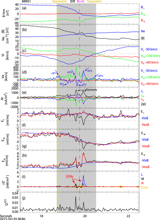
Figure A1. Two EDRs in an IDR observed by MMS1. (a) Three components of the magnetic field; (b) total magnetic field and electron density; (c) ion bulk velocities; (d) electron bulk velocities; (e) current densities calculated from plasma moments, Jp = en(vi − ve ); (f)–(h) three components of the measured electric field (black), −vi × B (blue), −ve × B (red); (i) energy dissipation J · (E + ve × B); and (j) electron nongyrotropy Q0.5. The two yellow dashed lines mark the two separatrices.
Download figure:
Standard image High-resolution image
Figure A2. Two EDRs in an IDR observed by MMS3. (a) Three components of the magnetic field; (b) total magnetic field and electron density; (c) ion bulk velocities; (d) electron bulk velocities; (e) current densities calculated from plasma moments, Jp = en(vi − ve ); (f)–(h) three components of the measured electric field (black), −vi × B (blue), −ve × B (red); (i) energy dissipation J · (E + ve × B); and (j) electron nongyrotropy Q0.5. The two yellow dashed lines mark the two separatrices.
Download figure:
Standard image High-resolution image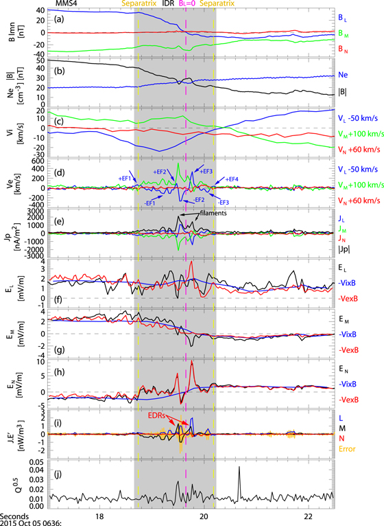
Figure A3. Two EDRs in an IDR observed by MMS4. (a) Three components of the magnetic field; (b) total magnetic field and electron density; (c) ion bulk velocities; (d) electron bulk velocities; (e) current densities calculated from plasma moments, Jp = en(vi − ve ); (f)–(h) three components of the measured electric field (black), −vi × B (blue), −ve × B (red); (i) energy dissipation J · (E + ve × B); and (j) electron nongyrotropy Q0.5. The two yellow dashed lines mark the two separatrices.
Download figure:
Standard image High-resolution image
Figure A4. Schematic view of a deformed EDR. We consider two cases: (a) and (b) are for the EDR deformed in the
L
–
N
plane, while (c) and (d) are for the EDR deformed in the
M
–
N
plane. Panels (a) and (c) show the cartoon for a deformed EDR and the spacecraft trajectory across the EDR. Panels (b) and (d) display the profiles of BL
and  along the trajectory of the spacecraft as it crosses the EDR shown in (a) and (c), respectively. If the spacecraft crosses this deformed EDR oblique to
N
due to the background flow in
L
or
M
, it might cross the deformed EDR twice. In these cases, the spacecraft may record two peaks in
along the trajectory of the spacecraft as it crosses the EDR shown in (a) and (c), respectively. If the spacecraft crosses this deformed EDR oblique to
N
due to the background flow in
L
or
M
, it might cross the deformed EDR twice. In these cases, the spacecraft may record two peaks in  similar to the MMS observation. However, the second crossing of the EDR must be manifested as a decrease of BL
to zero, which is inconsistent with the nearly monotonic variation of BL
as MMS crossed the current sheet. Therefore, we believe it is unlikely that the observation of the two EDRs is caused by a single deformed EDR.
similar to the MMS observation. However, the second crossing of the EDR must be manifested as a decrease of BL
to zero, which is inconsistent with the nearly monotonic variation of BL
as MMS crossed the current sheet. Therefore, we believe it is unlikely that the observation of the two EDRs is caused by a single deformed EDR.
Download figure:
Standard image High-resolution image
Figure A5. Four MMS spacecraft observations of the reconnecting current sheet without time shift. (a) Total magnetic field; (b) electron number density; (c) electron perpendicular temperature; (d)–(f) three components of the current density; (g) total current density; and (h) L component of the electron bulk velocity and the half local electron Alfvén speed.
Download figure:
Standard image High-resolution image
Table A1. Parameters on the Two Sides of the Undisturbed Current Sheet and the Mirror-modulated Current Sheet
| Initial Undisturbed Current Sheet (before the Growth of the Ion-Mirror Mode) | ||
|---|---|---|
| Time range | 2015-10-05/06:34:00.00 to 2015-10-05/06:36:20.00 UT | 2015-10-05/06:36:20.00 to 2015-10-05/06:37:00.00 UT |
| Magnetic field (GSE) | [X, Y, Z, total] = [−9.8, 30.9, 9.5, 33.8] nT | [X, Y, Z, total] = [−3.5, 11.9, −15.7, 20.1] nT |
| Plasma β (Pi/Pb) | 6.0 | 14.6 |
| Mirror-modulated current sheet | ||
| Time range | 2015-10-05/06:36:15.00 to 2015-10-05/06:36:17.00 UT | 2015-10-05/06:36:22.00 to 2015-10-05/06:36:24.00 UT |
| Magnetic field (GSE) | [X, Y, Z, total] = [−5.7, 42.7, 23.8, 49.2] nT | [X, Y, Z, total] = [0.3, 9.3, −8.9, 12.8] nT |
| Plasma β (Pi/Pb) | 1.3 | 34.5 |
Download table as: ASCIITypeset image
Table A2. The Reconnecting Magnetic Field and Plasma Density Used to Estimate the Asymmetric Hybrid Alfvén Speed
| Strong B Side | Weak B Side | |
|---|---|---|
| Time | 2015-10-05/06:36:18.00 UT | 2015-10-05/06:36:21.00 UT |
| Reconnecting Magnetic field | BL1 = 35 nT | BL2 = −10 nT |
| Plasma density | N1 = 20 cm−3 | N2 = 30 cm−3 |
Download table as: ASCIITypeset image