


Abstract
Self-organized criticality describes a class of dynamical systems that maintain themselves in an attractor state with no intrinsic length or timescale. Fundamentally, this theoretical construct requires a mechanism for instability that may trigger additional instabilities locally via dissipative processes. This concept has been invoked to explain nonlinear dynamical phenomena such as featureless energy spectra that have been observed empirically for earthquakes, avalanches, and solar flares. If this interpretation proves correct, it implies that the solar coronal magnetic field maintains itself in a critical state via a delicate balance between the dynamo-driven injection of magnetic energy and the release of that energy via flaring events. All-sky high-cadence surveys like the Transiting Exoplanet Survey Satellite (TESS) provide the necessary data to compare the energy distribution of flaring events in stars of different spectral types to that observed in the Sun. We identified ∼106 flaring events on ∼105 stars observed by TESS at a 2 minute cadence. By fitting the flare frequency distribution for different mass bins, we find that all main-sequence stars exhibit distributions of flaring events similar to that observed in the Sun, independent of their mass or age. This may suggest that stars universally maintain a critical state in their coronal topologies via magnetic reconnection events. If this interpretation proves correct, we may be able to infer properties of magnetic fields, interior structure, and dynamo mechanisms for stars that are otherwise unresolved point sources.
Export citation and abstract BibTeX RIS

Original content from this work may be used under the terms of the Creative Commons Attribution 4.0 licence. Any further distribution of this work must maintain attribution to the author(s) and the title of the work, journal citation and DOI.
1. Introduction
The concept of self-organized criticality (Bak et al. 1988) describes a class of dissipative dynamical systems that remain at a critical point with no intrinsic length or timescale. The existence of the critical state requires a local instability, which occurs when some parameter exceeds its critical value and results in a dissipative transport process where this same parameter increases at neighboring sites. A simple physical analogy is a sand pile. As sand particles are added, the difference in height between neighboring sites on the pile increases. When the additional sand particles make the new height difference exceed a critical threshold, avalanche events occur. This system maintains a critical slope, representing a dynamical attractor that is insensitive to the initial conditions. This critical state is maintained via nonlinear avalanche events spanning all length scales triggered by perturbations.
While the sand pile analogy is simplistic by construction, self-organized criticality naturally manifests in a variety of physical systems. Applications have been found in hydrodynamical turbulence, forest fires and other percolation systems (Turcotte 1999), landslides (Bak et al. 1990; Turcotte et al. 2002), neuroscience (Ribeiro et al. 2010; Hesse & Gross 2014), climate fluctuations (Grieger 1992), rainfall (Andrade et al. 1998), accretion disks (Dendy et al. 1998), traffic jams (Nagel & Herrmann 1993), evolution (Bak & Sneppen 1993), extinction (Newman 1996), financial markets (Bak et al. 1997), and even Conway's game of Life (Bak et al. 1989), to name a noncomprehensive list. The theory also explains the Gutenberg–Richter (Gutenberg & Richter 1956) law for the distribution of earthquake energies (Bak & Tang 1989; Sornette & Sornette 1989; Olami et al. 1992),

where N is the number of earthquakes, E is the energy released in the earthquake (where the earthquake magnitude  ), and the power-law exponent 1.25 < α ∼ 1.5. A three-dimensional slip-stick model of tectonic events produces a critical exponent of α = 1.35 (Bak & Tang 1989), in reasonable agreement with the observed law. It is worth noting that scalar redistribution rules for the sand pile analogy have been generalized, and that the dynamics of the vectorial case are quantitatively similar to those for the scalar-field case (Robinson 1994).
Even the solar coronal magnetic field may reside in a self-organized critical state (Lu & Hamilton 1991). This hypothesis naturally explains the power-law dependence of the magnitude of solar flares, which is of the same form as Equation (1), where α ≈ 1.4 (Lu & Hamilton 1991). This characteristic exponent and the subsequent temporal clustering are universal between earthquakes and solar flares (de Arcangelis et al.2006).
Explosive events on the Sun are believed to be driven by the energy stored in twisted coronal magnetic field lines (Parker 1989). Such field configurations are generated through dynamo action in the fluid-dominated interior (Charbonneau 2010), and through convective and coriolis-driven vortical subsurface plasma flows (Parker 1955; Moffatt 1978; Longcope et al. 1998; Seligman et al.2014). The concentration of magnetic field lines can lead to the release and subsequent dissipation of energy via the process of magnetic reconnection (Sturrock et al. 1984). These reconnection events could be triggered when the angle, θ, between neighboring magnetic field vectors is greater than a critical value, θc . The reconnection event changes the angles for neighboring field lines and can trigger additional events (Sturrock et al. 1984; Parker 1988; Sturrock et al. 1990). When θ < θc , a sequence of metastable states develops, allowing for the buildup of non-potential magnetic energy in the form of twisted field lines. Thus, this configuration satisfies all the requirements for a self-organized critical system, if given a source for energy injection.
Recent studies have begun to explore if flaring events on stars across all spectral types and evolutionary stages exhibit the same power-law distribution as the Sun. This finding may suggest that other stars also maintain self-organized critical states in their coronal magnetic fields. However, this hypothesis has previously been difficult to test due to (i) the lack of a long observational baseline to capture a sufficient number of flaring events; (ii) the lack of observations of a large number of stars across spectral types; and (iii) the difficulty in observing, identifying, and characterizing flares, especially those with low amplitudes relative to instrumental noise. Extra-solar surveys such as Kepler/K2 (Borucki et al. 2010) and the Transiting Exoplanet Survey Satellite (TESS; Ricker et al. 2015) have provided solutions to (i) and (ii). These missions have provided unprecedented, high-precision, long-baseline light curves for hundreds of thousands of stars.
Aschwanden & Güdel (2021) identified a power-law dependence with α = 1.824 ± 0.007 in the cumulative distribution of flaring events observed in a set of stars across stellar types observed with Kepler. This suggests that the self-organized critical state observed in the solar corona is ubiquitous. However, the published Kepler catalogs tend to be biased toward high-amplitude flares because of the inefficiency at identifying low-amplitude events of implemented flare-detection algorithms. Moreover, these catalogs are contaminated with other features easily mistaken for flaring events, such as rapidly rotating or variable stars (Davenport 2016). Further complicating matters, the flares that are both observed and identified correctly in Kepler are not fully temporally resolved due to the 30 minute cadence of the observations. The TESS mission has recently provided 2 minute cadence light curves for ∼200,000 of the nearest and brightest stars. These data provide a full sample of spectral types across the main sequence to search for temporally resolved flaring events (Günther et al. 2020).
Additionally, machine-learning techniques curated to identify flares in TESS short cadence data have been developed to rectify issue (iii). These novel techniques are capable of identifying low-amplitude flares with high fidelity (Feinstein et al. 2020b; Vida et al. 2021). This combination of unprecedented data and efficient identification techniques provides a new opportunity to expand the hypothesis of self-organized criticality in the solar corona to a sample of stars representative of the galactic census of spectral types and ages. In this Letter, we provide a complementary search for indications of self-organized criticality in flaring events observed by TESS, using our newly created catalog of stellar flares from two years of data (M. N. Günther et al. 2022, in preparation).
2. Observations with TESS
NASA's five-year TESS mission is currently performing time series photometry of ∼90% of the sky (Ricker et al. 2015). The survey observes in 24° × 96° sectors for ∼27 days at a time. During its primary 2 yr mission, TESS observed ∼200,000 pre-selected stars at a 2 minute cadence across both ecliptic hemispheres. TESS has been providing an unprecedented data set at high temporal resolution with which to identify flaring events across stellar spectral types and ages. The light curves used in this study were processed by the Science Processing Operations Center (SPOC) pipeline operated at the NASA Ames Research Center, which performs optimized aperture selection and systematics detrending (Jenkins et al. 2016). We applied pipeline-assigned quality flags to mask contaminated 10 regions of the light curves.
2.1. Flare Identification
As mentioned previously, flare identification in time series photometric data has proven challenging. Previous methods of flare identification have relied on detrended, or "cleaned," light curves and have heuristics for outlier detections. However, detrending often removes low-amplitude flares entirely, and the outlier heuristics (e.g., Chang et al. 2015) are biased toward the identification of only the highest amplitude events. Conversely, more lenient heuristics produce a significant number of false positive events.
Neural networks are a class of supervised machine-learning algorithm optimized for visualization problems such as identifying features in one-dimensional time series (e.g., Ansdell et al. 2018; Pearson et al. 2018; Vida et al. 2021) or images (e.g., Tanoglidis et al. 2021). Here, we used the convolutional neural networks (CNNs) developed in Feinstein et al. (2020b), 11 which are accompanied by the open-source software package stella (Feinstein et al. 2020a) and are easily scalable to a large number of TESS 2 minute light curves. stella is unique in that it provides a "probability" that any given cadence in a light curve is or is not part of a flaring event. We ran all 2 minute TESS light curves through 10 pre-trained stella models and averaged the probability outputs for our final catalog of flaring events. We require a probability ≥ 0.9 for an event, meaning the event has a 90% probability of being a true flare. We provide upper and lower limits by only including flaring events with a probability ≥ 0.50 and ≥ 0.99, respectively.
While stella recovers a high percentage of real flaring events, it was trained on the relatively small data set presented in Günther et al. (2020), with limited examples of contaminating features such as variable and eclipsing binary stars and noisy light curves. In M. N. Günther et al. (2022, in preparation) and this study, we therefore apply four quality-control filters to the stella outputs, mitigating the risk of false positives:
- 1.Signal-to-noise ratio filter: This filter removes any false positives originating from the increased photon noise of faint targets. To do this, we estimated the root-mean-square (rms) noise of a given light curve. We first removed any variability using a biweight filter with a window size of 20 minutes and then took the rms of the flattened light curve. We required stellar flare candidates to have an amplitude of ≥3× rms noise.
- 2.Outliers: This filter removes flaring events that appear in limited data points. We removed any flares with a fitted duration of ≤4 minutes which corresponds to 2 TESS data points.
- 3.Eclipsing binaries (EBs): This filter removes false positives originating from EBs, where the ingress and egress of the eclipse events could be misclassified as flare candidates. For this purpose, we use the entire TESS threshold-crossing-event (TCE) catalog provided by the SPOC pipeline. We check if the flare peak times are associated with known eclipses. If a flare candidate falls within the eclipse window (approximated as 3 times the TCE duration), we remove the flare from the catalog.
- 4.Variability/rotation: This filter removes false positives originating from the peaks of fast-variable and fast-rotating targets. If the target has ≥10 flares, we compute a Lomb–Scargle periodogram of the target light curve and of the affiliated probability time series. If the variability detected from each data set is within 2 days and has a false-alarm probability <0.05, all flares from this target are removed.
After these filters are applied, we are left with a catalog of Nflares = 958,659 originating from Nstars = 161,836 for our analysis. A summary of our catalog is presented in Table 1 and the full catalogs are made available in M. N. Günther et al. (2022, in preparation). We calculate the flare rate per star, βstar, as

where N is the number of flares for a given star, pi is the stella probability for a given flare indexed by i, and τobs is the total observed time. An overview of the flare rates for all stars in our sample is presented in Figure 1 on a Gaia color–magnitude diagram. Here, we use Bp − Rp as our color and the absolute Gaia G magnitude MG . It is evident that stars with the highest flare rates (≥0.3 day−1) fall along the upper edge of the main sequence (meaning they are brighter, i.e., have a lower absolute magnitude, than other stars of that given color). This trend could be indicative of binary star systems (Hurley & Tout 1998) or young, metal-rich stars (Kotoneva et al. 2002). For our analysis, we only account for stars along the main sequence and the red giant branch (RGB; stars that fork to the right at 1 ≤ Gaia Bp − Rp and MG ≤ 2.5).
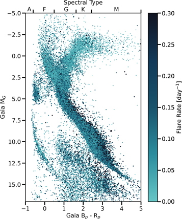
Figure 1. A color–magnitude diagram (Gaia Bp − Rp color and absolute Gaia G magnitude, MG ) for our sample colored by flare rate. The flare rate was calculated by weighting each flare by its output "probability" from stella. Here, we accounted for all identified flares, not just flares with probabilities ≥ 0.9. Stars toward the top of the main sequence tend to have higher flare rates. This trend could be due to being young and metal-rich or being binaries.
Download figure:
Standard image High-resolution imageTable 1. Sample Summary Statistics
| Bp − Rp | Mass (M⊙) | Nstars |

|
|---|---|---|---|
| [2.78, 4.86] | [0.05, 0.3) | 9241 | 59,150 |
| [2.13, 2.78) | [0.3, 0.5) | 20,124 | 108,963 |
| [1.21, 2.13) | [0.5, 0.8) | 17,914 | 139,445 |
| [0.327, 1.21) | [0.8, 1.7) | 85,609 | 571,556 |
| [−0.12 , 0.327) | [1.7, 3.0] | 3770 | 20,447 |
| Red Giant Branch | [0.8, 1.8] | 5157 | 10,965 |
Note. The relationship between Gaia Bp − Rp and stellar mass was taken from Pecaut & Mamajek (2013). Red giant branch stellar masses are adopted from Wu et al. (2019).
Download table as: ASCIITypeset image
3. Measured Flare Rates
We present our measured flare frequency distributions (FFDs) as a function of stellar mass and flare amplitude (Figure 2). The mass bins were selected based on spectral types/changes in interior stellar structure: stars with masses M/M⊙ ≲ 0.3 are fully convective (Dorman et al. 1989; Chabrier & Baraffe 1997), stars with masses 0.3 < M/M⊙ ≲ 1.7 have convective exteriors and radiative interiors, and stars with masses M/M⊙ > 1.7 have radiative exteriors and convective interiors (Heger et al. 2000). We present these results in flare-amplitude space, compared to energy, to remove any additional errors resulting from estimating stellar luminosities. In theory, the flare energy is more directly relevant to the predicted self-organized critical state. However, in practice, the uncertainty in mass and luminosity of each star makes the amplitude a more reliable quantity.

Figure 2. The cumulative flare frequency distributions (FFDs) in our sample of stars binned by the flare amplitude and subdivided into different mass bins; the slope, α, and error is given in the upper-right corner of each subpanel. The bins are the FFD for flares with a probability ≥0.9. The upper and lower errors on the FFD are defined as flares with probability ≥0.99 and ≥0.5. All bins exhibit clear power laws, although some bins are incomplete for low-amplitude flares (e.g., 0.05 ≤ M/M⊙ ≤ 0.3) or high-amplitude flares (e.g., red giant branch).
Download figure:
Standard image High-resolution imageWe measure the slope of each distribution, α, and associated error using a Markov Chain Monte Carlo (MCMC) approach with emcee (Goodman & Weare 2010; Foreman-Mackey et al.2013). Our MCMC chains were initialized with 300 walkers and ran for 5000 steps. After visual inspection, we removed the first 800 burn-in steps and verified our chains converged, following the method of Geweke (1992). We present our FFDs and measured slope with error in Figure 2. The black line in each subpanel represents our fits that excluded incomplete bins. For example, several of the low-amplitude bins are incomplete because of (1) observational constraints such as the cadence of the observations or stellar/systematic noise in the light curves and (2) limitations imposed by our definition of flare events in TESS data (see itemized list of filters in Section 2.1 for more details). Although it is theoretically feasible to quantify the incompleteness via injection-recovery tests, Feinstein et al. (2020b) stated that this method does not accurately represent the performance of the stella CNNs. This limitation is due to the uncertainty in generating synthetic flare photometric models, and the subsequent differences in real and injected flares. We note that Feinstein et al. (2020b) demonstrated that ≈80% of flares with amplitudes ≤5% were recovered, corresponding to the first four bins of each panel in Figure 2. For most of our sub-samples, these bins were not used for the fit. Finally, we note that the choice of excluded bins (here due to incompleteness) can affect the power-law slopes resulting from the fits.
We find that the FFDs for stars with masses 0.3 ≤ M/M⊙ ≲ 3.0 appear as featureless power laws. The measured slopes are consistent with models of flaring activity as self-organized critical systems (α ≈ 1.4 Lu & Hamilton 1991) and with that measured for the Sun (α = 1.65 ± 0.1; de Arcangelis et al. 2006).
Our lowest mass bin (0.05 ≤ M/M⊙ ≤ 0.3) and our sample of RGB stars do not follow the same trends. Stars with 0.05 ≤ M/M⊙ ≤ 0.3 show a featureless power law for flare amplitudes ≥5%; while power laws are indicative of a self-organized critical state, the difference in interior structure may result in a shallower flare rate (here, α ∼ 1). The most energetic flares have historically been observed on low-mass stars in this bin (Feinstein et al. 2020b). It is possible that because these stars are fully convective and therefore have larger convective cells than other main-sequence stars, they produce more energetic flares. Similarly, red giants have larger convective cells and display even shallower slopes in their FFD. We also note that our bins of stars with 1.7 < M/M⊙ ≤ 3.0 and RGB stars have the fewest number of flares (Table 1) and while we are able to measure the slopes of these FFDs, they are incomplete to the lowest and highest amplitude flares.
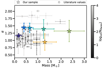
Finally, in Figure 3 we compare our measured FFD slopes from our cumulative distribution to those presented by previous authors. Previous studies used an order of magnitude fewer flaring events than we did and tend to report shallower slopes (α ∼ 1) than the ones measured here. The variation in measured slopes arises based on sample size/selection, and the cadence of the analyzed data (from 1 to 30 minute cadence). This discrepancy may also be explained by fewer high-amplitude events in the samples given their rarity. In this study, we also extended our measurement of flare rates to include a broader stellar mass and evolutionary stage range.
Figure 3. Comparison of measured cumulative distribution flare rate slopes, α, as a function of stellar mass. Our rates are plotted as stars. Literature values are plotted as circles and colored by the number of flares in the given sample; they range from 1 to 104 stars (Shibayama et al. 2013; Howard et al. 2019; Ilin et al. 2019, 2021; Lin et al. 2019; Yang & Liu 2019; Feinstein et al. 2020b; Günther et al. 2020; Raetz et al. 2020; Aschwanden & Güdel 2021). The highest-mass stars have higher flare rate indices (light green) than previously measured. Our RGB star (yellow) slope is within 1σ of that of main-sequence stars in the same mass range. The remaining data points fall within the expected range of self-organized critical systems. We estimate the masses of our RGB stars using results from Wu et al. (2019).
Download figure:
Standard image High-resolution image
4. Conclusions and Future Work
In this Letter, we analyzed the light curves of 161,836 stars that were observed by TESS at a 2 minute cadence. These light curves were processed and searched for flares using a novel machine-learning algorithm (Feinstein et al. 2020a, 2020b), resulting in a catalog of ∼106 flaring events (M. N. Günther et al. 2022, in preparation). In Figure 1, we show how the flare rate changes as a function of location on a color–magnitude diagram. In Figure 2, we show the flare frequency distribution of stars as a function of stellar mass and compare it to that found in the literature (Figure 3). Main-sequence stars with M/M⊙ ≥ 0.3 exhibit power-law distributions of flare rates with slopes that are characteristic of self-organized critical systems (α ≈ 1.4). The resulting indices are somewhat smaller for stars with M/M⊙ <0.3 and for red giant stars (which have slopes α ∼ 1). This discrepancy may be due to differences in the interior structure of these stars, which have larger convective cells compared to other main-sequence stars, or due to the incompleteness of our sample of flares on red giant branch stars.
Although the measured slopes of the flare rates show some scatter, the results of this paper indicate a high degree of universality. In the working picture that emerges, subsurface convective regions efficiently inject sufficient energy in the form of twisted magnetic fields near the stellar surface. Subsequent reconnection events then act to produce flares and maintain the magnetic field topology in a self-organized critical state. For completeness, we note that power-law distributions can arise through a variety of mechanisms (Newman 2005), not only via self-organized criticality, so that additional theoretical modeling of these systems is indicated.
TESS will continue to observe ∼90% of the sky for the next three years. The full-frame images that observe ∼106 stars per month will soon increase to a higher cadence, making flare identification more feasible for an order of magnitude more stars than presented herein. This increase should further complete the distribution of the rarest, high-energy events. The timing of sympathetic flares after a "main" flare event (defined by some amplitude threshold), can be used to further investigate if these systems maintain a self-organized critical state, as was observed for the Sun and for earthquake aftershocks (de Arcangelis et al. 2006). Due to the short baseline of TESS (∼1 month), this study may only be truly complete for stars within TESS's continuous viewing zone, those that get ∼1 yr of continuous observations. Such a study could also be completed with the already available Kepler light curves, which have a baseline of 4 yr to search for the timing of sympathetic flares.
We thank Mark Krumholz, Fausto Cattaneo, Adrian Price-Whelan, Jacob Bean, Leslie Rogers, and Konstantin Batygin for insightful conversations. We thank the anonymous referee and our scientific editor, Manolis K. Georgoulis, for helpful comments and suggestions. A.D.F. acknowledges support from the National Science Foundation Graduate Research Fellowship Program under grant No. (DGE-1746045). M.N.G. acknowledges support from MIT's Kavli Institute as a Juan Carlos Torres Fellow and from the European Space Agency (ESA) as an ESA Research Fellow. This research has made use of NASA's Astrophysics Data System Bibliographic Services. This work made use of open-source Python packages (Hunter et al. 2007; Astropy Collaboration et al. 2013, 2018; Harris et al. 2020; Virtanen & Contributors 2020; Feinstein et al. 2020a). This paper includes data collected by the TESS mission. Funding for the TESS mission is provided by the NASA's Science Mission Directorate.
Footnotes
- 10
Contamination can originate from cosmic rays, reaction-wheel desaturation events, and other spacecraft sources. For more information, see Table 28 in Tenenbaum & Jenkins (2018).
- 11
The pre-trained CNNs are available online: https://archive.stsci.edu/hlsp/stella.