


Abstract
Recent Parker Solar Probe (PSP) observations of inner heliospheric plasma have shown an abundant presence of Alfvénic polarity reversal of the magnetic field, known as "switchbacks." While their origin is still debated, their role in driving the solar wind turbulence has been suggested through analysis of the spectral properties of magnetic fluctuations. Here, we provide a complementary assessment of their role in the turbulent cascade. The validation of the third-order linear scaling of velocity and magnetic fluctuations in intervals characterized by a high occurrence of switchbacks suggests that, irrespective of their local or remote origin, these structures are actively embedded in the turbulent cascade, at least at the radial distances sampled by PSP during its first perihelion. The stronger positive energy transfer rate observed in periods with a predominance of switchbacks indicates that they act as a mechanism injecting additional energy in the turbulence cascade.
Export citation and abstract BibTeX RIS

Original content from this work may be used under the terms of the Creative Commons Attribution 4.0 licence. Any further distribution of this work must maintain attribution to the author(s) and the title of the work, journal citation and DOI.
1. Introduction
The Parker Solar Probe (PSP) spacecraft (Fox et al. 2016) has recently provided valuable measurements of solar wind particles and fields in the inner heliosphere. Aiming at reaching as close as 9.86 solar radii from the solar surface, these observations represent a unique tool to address several open questions concerning the heliosphere. Among those, understanding the origin and the evolution of turbulence is crucial for a correct description of the dynamics of the heliospheric plasma and of the Sun–Earth relation (Matthaeus & Velli 2011; Usmanov et al. 2011; Bruno & Carbone 2013; Smith & Vasquez 2021; Telloni et al. 2021).
An interesting feature observed by PSP is the broad presence of sudden reversals of the interplanetary magnetic field vector, also called switchbacks (Bale et al. 2019). Observed from previous measurements from other spacecraft (Yamauchi et al. 2004), these structures are increasingly visible closer to the Sun. The characteristics of the switchbacks have been studied in depth using PSP data as well as numerical simulations (e.g., Horbury et al. 2020; Bandyopadhyay et al. 2021), yet their origin is still being debated and several models, not mutually exclusive, have been proposed. For example, it is thought that switchbacks could be the signature of flux ropes produced by interchange reconnection in the solar corona (Fisk & Kasper 2020; Sterling & Moore 2020; Zank et al. 2020; Drake et al. 2021; Liang et al. 2021) or that they might be associated with the motion of magnetic field footpoints from the slow to the fast wind sectors (Schwadron & McComas 2021). Magnetohydrodynamic (MHD) numerical simulations suggest they may be Alfvénic structures originated in the lower corona and propagating out in the heliosphere (Matteini et al. 2015; Tenerani et al. 2020), or may be related to velocity shear-driven dynamics (Landi et al. 2006; Ruffolo et al. 2020). A different approach considers switchbacks as self-consistently generated during the solar wind expansion of turbulent fluctuations (Squire et al. 2020). The switchback occurrence characteristics observed by PSP were used to support their origin in the transition region rather than in situ (Bale et al. 2021; Fargette et al. 2021; Mozer et al. 2021).
One of the most intriguing questions concerns the relationship between the presence of switchbacks and turbulence. Indeed, these structures can either be seen as superposed to preexisting turbulence, or as dynamically connected to its onset, perhaps acting as an additional energy injection source for the nonlinear turbulent cascade. This latter scenario was investigated in Dudok de Wit et al. (2020), in which the spectral properties of magnetic fluctuations are studied separately for periods of high and low incidences of switchbacks. In their work, these authors show that the magnetic spectra are fully developed to a Kolmogorov-like scaling f−3/2 only in the intervals largely populated by switchbacks. On the contrary, the intervals with fewer switchbacks showed a reduced Kolmogorov inertial range toward the higher frequencies, the lower ones being characterized by a 1/f uncorrelated noise typical of the evolving solar wind (Bavassano et al. 1982; Verdini et al. 2012; Chandran 2018; Matteini et al. 2018). The interpretation provided in Dudok de Wit et al. (2020) is that the quiet samples have underdeveloped turbulence, while switchbacks are associated with a more developed turbulent state of the solar wind plasma. According to that, switchbacks would likely play an active role in driving the turbulence, accelerating its evolution as the solar wind is expanding. Similar conclusions were drawn in separate studies (Bourouaine et al. 2020). Using PSP, Ulysses, and Helios data, Tenerani et al. (2021) provided a comprehensive description of the radial evolution of switchbacks, suggesting that their dynamics is a complex process that may include the decay through turbulent fluctuations, but also the generation in situ in the inner heliosphere. Other analyses have indicated that switchbacks are sites of enhanced intermittency (Perrone et al. 2020; Martinović et al. 2021), while the sharp boundary layers separating the switchbacks from the remnant plasma flow are characterized by an intense current and electric field (Krasnoselskikh et al. 2020). Finally, an increased parallel temperature in switchbacks has been also observed, suggesting a possible role of microinstabilities (Larosa et al. 2021; Woodham et al. 2021).
Most of these observations are consistent with the general understanding that, for increasing distance from the Sun, the turbulent power-law spectrum expands toward larger scales (Bavassano et al. 1982; Bruno & Carbone 2013; Chen et al. 2020). However, spectral properties may be misleading, as it is not possible to unequivocally ascribe the Kolmogorov-like power-law scaling to the presence of a turbulent cascade. For example, it is universally observed that turbulence is associated with intermittency (Kolmogorov 1962), as is routinely observed in solar wind measurements (Sorriso-Valvo et al. 1999; Bruno & Carbone 2013). A standard way for characterizing the intermittency of a field ϕ (ϕ being, for example, a velocity or magnetic field component) is by means of the scale-dependent increments Δϕ = ϕ(t + Δt) − ϕ(t), which account for the presence of gradients on a timescale Δt (Anselmet et al. 1984). Intermittency is related to the scale-dependent shape of the probability distribution function of the increments Δϕ (Castaing et al. 1990). This, additionally, implies the existence of nonvanishing odd moments. In particular, a scaling law can be derived for the third-order moment directly from the dynamical MHD equations, as the conservation law of the appropriate inviscid invariants (de Karman & Howarth 1938; Danaila et al. 2001). Such a relation, known in the MHD description as the Politano–Pouquet (PP) law (Politano & Pouquet 1998; Carbone et al. 2009), establishes that under the hypothesis of homogeneity, stationarity, local isotropy, and incompressibility, in the turbulent inertial range the mixed third-order moment of the increments of velocity (
v
) and magnetic field (in velocity units,  , with
B
the magnetic field vector and ρ the plasma mass density) is a linear function of the scale Δt. Moreover, the proportionality coefficient is related to the mean energy transfer rate of the turbulent cascade. This can be written as
, with
B
the magnetic field vector and ρ the plasma mass density) is a linear function of the scale Δt. Moreover, the proportionality coefficient is related to the mean energy transfer rate of the turbulent cascade. This can be written as
Here Δ v and Δ b are scale-dependent vector increments of the plasma velocity and magnetic field, as defined above; ΔvR = vR (t + Δt) − vR (t) and ΔbR = bR (t + Δt) − bR (t) are velocity and magnetic field longitudinal increments measured in the sampling direction R; ε is the mean energy transfer rate; and brackets indicate ensemble average. Note that the solar wind speed Vsw is used for switching between space scales, ℓ, and timescales, Δt, through the Taylor hypothesis, ℓ = VswΔt (Taylor 1938). This also results in the reversal of the sign in the left-hand side of Equation (1) with respect to the traditional formulation in terms of spatial increments. The PP law is a fundamental relation for MHD turbulence, since it describes the energy cascade and ultimately allows us to estimate the energy that will be dissipated at small scales. It is particularly relevant for solar wind turbulence, where the collisionless processes responsible for removing the energy at the bottom of the nonlinear cascade are not yet fully understood (Chen et al. 2019; Sorriso-Valvo et al. 2019; Matthaeus et al. 2020; Smith & Vasquez 2021). The linear relation (1) has been observed in various regions of the heliosphere, for different conditions of the space plasma, confirming the turbulent nature of their dynamics and providing an estimate of the energy transfer rate (MacBride et al. 2005; Sorriso-Valvo et al. 2007; Marino et al. 2008; Smith et al. 2009; Stawarz et al. 2010; Coburn et al. 2012; Bandyopadhyay et al. 2018; Hadid et al. 2018; Andrés et al. 2019; Bandyopadhyay et al. 2020; Sorriso-Valvo et al. 2021).
In this Letter, the PP law is used to characterize the turbulent cascade in intervals of solar wind with a variable occurrence of the switchbacks. Observations will help assess the role of the switchbacks in the radial evolution of turbulence and may contribute to understanding their origin.
2. Data and Methodology
PSP collects high-resolution data within the encounter phase of its orbit, when the distance between the spacecraft and the Sun is less than 0.25 au (Guo et al. 2021). Here, we use data from the first solar encounter. We use magnetic field data from the FIELDS fluxgate magnetometer (MAG; Bale et al. 2016, 2019. In particular, L2 full-cadence magnetic field data from the files "PSP_FLD_L2_MAG_RTN" are used. Ion density and velocity are obtained from Level-3 data recorded by the PSP/SWEAP Solar Probe Cup (SPC; Case et al. 2020; Kasper et al. 2016, 2019). Only "good quality" (marked so by flags) "Moments" data from L3 files (e.g., "PSP_SWP_SPC_L3i") are used.
The measurements used for this work are shown in the first three panels of Figure 1. We used the PSP measurements to compute the time series of the unaveraged mixed third-order increments appearing in Equation (1), LET(Δt) ≡ ΔvR (∣Δ v ∣2 + ∣Δ b ∣2) − 2ΔbR (Δ v · Δ b ). This is a local proxy that can give information on the local contribution to the energy transfer rate (Sorriso-Valvo et al. 2018, 2019), and is shown in the second to last panel of Figure 1.

Figure 1. Overview plot of the first PSP encounter. From top to bottom: proton velocity v p (500 s average); magnetic field B (500 s average); proton density np (500 s average); switchback parameter z (gray line) and its average values in 6 hr running windows 〈z〉 (color-coded points, see the legend); local energy transfer rate proxy LET estimated for Δt = 16 s; mean energy transfer rate ε (color-coded points, see the legend), along with the radial distance from the Sun in solar radii units R/R⊙ (black line).
Download figure:
Standard image High-resolution imageFor the identification of switchbacks, as introduced by Dudok de Wit et al. (2020), we used the parameter  , where
  is the angle of deflection of the local magnetic vector
B
with respect to the mean field 〈
B
〉 estimated over 6 hr intervals. The resulting time series is shown in the fourth panel of Figure 1. From a visual inspection, it can be observed that the amplitude of the LET fluctuations is larger in the central and left portions of the sample, where switchbacks appear more frequently (larger z). The time series of the parameter z is then used to manually select intervals of consistently high or low occurrences of switchbacks. In order to ensure that all selected intervals are sufficiently long enough to allow statistical analysis, we impose a minimum length of 3 hr for the selection. This choice is based on the typical correlation timescale of the magnetic fluctuations τc
≲ 1 hr, estimated for the first encounter (Parashar et al. 2020; Bandyopadhyay et al. 2020), so that no intervals are shorter than 3τc
. Using the above procedure, we have initially selected six intervals of high incidences of switchbacks (S), and six quiet intervals with no or very few switchbacks (Q). Their position is shown in the fourth panel of Figure 1, where the mean value of 〈z〉 is indicated by purple (S) and green (Q) symbols, each located at the center of the respective interval. Alternatively, in order to perform a more complete analysis, the whole data set has been divided into 40 nonoverlapping 6 hr running windows (R), each one characterized by a given value of 〈z〉, shown by the blue symbols in the fourth panel of Figure 1. The choice of the window size was based, again, on the aforementioned correlation timescale estimate and on similar values used in previous works (Chen et al. 2020; Bandyopadhyay et al. 2020).
is the angle of deflection of the local magnetic vector
B
with respect to the mean field 〈
B
〉 estimated over 6 hr intervals. The resulting time series is shown in the fourth panel of Figure 1. From a visual inspection, it can be observed that the amplitude of the LET fluctuations is larger in the central and left portions of the sample, where switchbacks appear more frequently (larger z). The time series of the parameter z is then used to manually select intervals of consistently high or low occurrences of switchbacks. In order to ensure that all selected intervals are sufficiently long enough to allow statistical analysis, we impose a minimum length of 3 hr for the selection. This choice is based on the typical correlation timescale of the magnetic fluctuations τc
≲ 1 hr, estimated for the first encounter (Parashar et al. 2020; Bandyopadhyay et al. 2020), so that no intervals are shorter than 3τc
. Using the above procedure, we have initially selected six intervals of high incidences of switchbacks (S), and six quiet intervals with no or very few switchbacks (Q). Their position is shown in the fourth panel of Figure 1, where the mean value of 〈z〉 is indicated by purple (S) and green (Q) symbols, each located at the center of the respective interval. Alternatively, in order to perform a more complete analysis, the whole data set has been divided into 40 nonoverlapping 6 hr running windows (R), each one characterized by a given value of 〈z〉, shown by the blue symbols in the fourth panel of Figure 1. The choice of the window size was based, again, on the aforementioned correlation timescale estimate and on similar values used in previous works (Chen et al. 2020; Bandyopadhyay et al. 2020).
Finally, the scale-dependent mixed third-order moment Y(Δt) given by the PP law (1) was estimated by ensemble averaging the LET parameter over each of the intervals defined above (either Q, S, or R).
3. Results
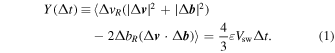
Figure 2 shows four examples of mixed third-order moment scaling in two S (purple) and two Q (green) intervals. Open and filled symbols refer to positive and negative values of Y, respectively (negative values were plotted in absolute value to allow for a logarithmic y-axis). The moments were rescaled by the factor 3/4Vsw in order to account for differences in the solar wind bulk speed in each interval, which is needed to correctly determine the energy transfer rate through the Taylor hypothesis. A linear scaling range is visible for 11 of the 12 manually selected intervals (S and Q), and in 63% of the running intervals (R). This observation confirms that the turbulent cascade is active, and the turbulence is at least moderately developed, in most of the solar wind intervals, irrespective of the presence or absence of switchbacks. In the case of S intervals, this observation demonstrates that switchbacks are part of the dynamical processes involved in the turbulent cascade. However, determining whether they are generated by the turbulence or rather they act as a possible driver for the observed nonlinear cascade remains to be clarified. For the Q intervals, the observation suggests that the turbulence is sufficiently developed to generate a cascade, despite previous observations of shallower spectra (Dudok de Wit et al. 2020) and reduced intermittency (not shown) seeming to suggest otherwise.
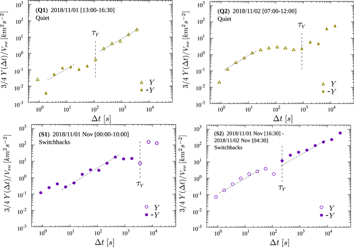
Figure 2. Examples of the Politano–Pouquet law (1) in four samples of PSP data. The third-order moment is normalized to the factor 3/(4Vsw), in order to account for variations in the solar wind speed used in the Taylor transformation. Purple and green symbols refer to S and Q intervals, respectively. Open and filled symbols indicate positive and negative values, respectively. Negative values have been sign-inverted to be represented in the logarithmic axis. The dashed line is a linear function shown for reference. Vertical lines indicate the timescale τY at which a sign reversal is observed.
Download figure:
Standard image High-resolution imageIn the four examples given in Figure 2, and in some of the remaining Q or S intervals, sign reversals of the mixed third-order moment are detected, shown as well-defined transitions from open to filled symbols (or vice versa). According to the standard interpretation of the cascade sign, and after considering the sign reversal due to the Taylor hypothesis transformation, positive and negative Y must be associated with direct and inverse cascades, respectively (Smith et al. 2009). However, the observation of the linear scaling is challenging, and the possible presence of local inhomogeneities results in possible ambiguities in the determination of its sign. This may represent a bias for the unambiguous interpretation of the sign as the definite direction of the cascade (Bandyopadhyay et al. 2018; Hadid et al. 2018; Sorriso-Valvo et al. 2021). Though, for statistically converging solar wind samples the sign emerging from averages of the local mixed third-order moment is likely to provide a robust indication of the energy flux direction.
For example, in the S2 case (bottom right panel of Figure 2), a change of sign is observed around Δt ≃ 220 s, with Y passing from positive at smaller scales to negative at larger scales. This could be interpreted as an energy source present at such a scale, feeding simultaneously a direct cascade toward smaller scales and an inverse cascade toward larger scales. Note that dual-cascade regimes have been observed in anisotropic fluid systems, in the presence of waves (Marino et al. 2013; Pouquet & Marino 2013; Marino et al. 2015a, 2015b; Pouquet et al. 2017). The switchbacks could be possibly playing a role in driving the cascade. At a similar timescale, Δt ≃ 110 s, the Q1 sample (top left panel) also changes sign, but in the reversed order. In the other two examples the change occurs at a larger scale, of the order of 103 s, with only the smaller scales showing a scaling law. In order to support the robustness of the observed sign reversal, for each Q or S interval we have estimated the scale τY
at which a single, well-defined sign reversal was observed (such as in the four cases shown in Figure 2). Then, to determine whether the observed changes are related to changes in the dynamics, or simply to sign convergence issues, we look for characteristic scales in an alternative descriptor of the turbulent cascade. In particular, we make use of the scale-dependent flatness factor  . Here we use the standard ith-order structure functions Si
(Δt) = 〈ΔBi
〉 of the scale-dependent magnetic field magnitude increments ΔB(t, Δt) = B(t + Δt) − B(t) (Anselmet et al. 1984). Similar results were obtained for different magnetic components. The flatness describes the scale-dependent deviation from Gaussian of the distribution function of the increments. For intermittent turbulence, it is expected (Frisch 1995) and observed (Carbone & Sorriso-Valvo 2014) to behave as a negative power law of the timescale in the inertial range. Figure 3 shows examples of the four intervals already presented in Figure 2. A break of the power-law scaling represents a characteristic timescale τF
, of the order of the turbulence outer scale, which is indicated by a vertical line in each panel.
7
The left panel of Figure 4 shows that the two sets of timescales, τY
and τF
, are comparable in most of the samples where the sign reversal was observed.
8
This evidence suggests that the sign reversal is related to a characteristic scale of the flow, and is therefore informative of the dynamics.
. Here we use the standard ith-order structure functions Si
(Δt) = 〈ΔBi
〉 of the scale-dependent magnetic field magnitude increments ΔB(t, Δt) = B(t + Δt) − B(t) (Anselmet et al. 1984). Similar results were obtained for different magnetic components. The flatness describes the scale-dependent deviation from Gaussian of the distribution function of the increments. For intermittent turbulence, it is expected (Frisch 1995) and observed (Carbone & Sorriso-Valvo 2014) to behave as a negative power law of the timescale in the inertial range. Figure 3 shows examples of the four intervals already presented in Figure 2. A break of the power-law scaling represents a characteristic timescale τF
, of the order of the turbulence outer scale, which is indicated by a vertical line in each panel.
7
The left panel of Figure 4 shows that the two sets of timescales, τY
and τF
, are comparable in most of the samples where the sign reversal was observed.
8
This evidence suggests that the sign reversal is related to a characteristic scale of the flow, and is therefore informative of the dynamics.

Figure 3. Examples of the flatness F(Δt) scaling in the same four samples of PSP data as in Figure 2. Vertical lines indicate the timescale τF at which the power-law scaling breaks.
Download figure:
Standard image High-resolution image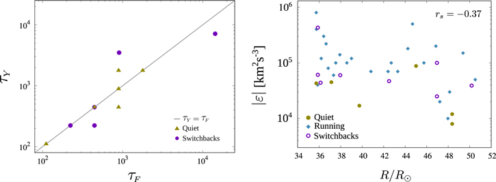
Figure 4. Left panel: timescales τY and τF of the sign reversal of the third-order moment Y and of the power-law break of the flatness F. The straight line indicates equal times, τY = τF . Note that at τY = τY ≃ 400 s there are four superposing points. Right panel: the magnitude of the energy transfer rate ∣ε∣ as a function of the radial distance R, for R, Q, and S intervals where the PP law was observed. The corresponding Spearman correlation coefficient between the two variables is indicated.
Download figure:
Standard image High-resolution imageHowever, because of the inherently delicate interpretation of the sign of the third-order averaged structure functions estimated from space plasma measurements, we decide not to discuss this point more in depth here, and leave it for further studies. In the following, even when we retain the sign information on the energy transfer rate ε, we shall keep in mind this caveat when interpreting the result.
For all the cases where a linear scaling was present over at least one decade of scales, a linear fit to Equation (1) was performed, obtaining the mean energy transfer rate ε. Note that if a sign reversal was observed at intermediate scales, fits have been performed on any of the segments complying with the requirement of one decade of scaling. In the bottom panel of Figure 1, the magnitude of the energy transfer rate ∣ε∣ is shown. Blue diamonds are used for the running-window intervals (εR ), green filled circles indicate quiet intervals (εQ ), and open purple circles indicate intervals with a high occurrence of switchbacks (εS ). Although the energy transfer rate is strongly fluctuating, a general trend is visible in the first half the PSP orbit, suggesting that larger values are observed closer to the Sun, while in the second half of the orbit the trend is less clear. This is in agreement with previous observations and with the independent estimates of a similar profile for the large-scale turbulent energy input (Bandyopadhyay et al. 2020). The observed trend can be highlighted by plotting ∣ε∣ as a function of the distance R, which is shown in the right panel of Figure 4. The nonlinear Spearman correlation coefficient between the two quantities is rs = − 0.37, indicating a general decrease with distance with low to moderate correlation. However, when considering positive scaling only, the correlation coefficient is considerably larger (−0.65). A more comprehensive study of all available PSP data will be necessary to explore the radial dependency of the turbulent cascade rate more in depth.
The possible dependence on the density of the switchbacks was investigated within each group of intervals. This was done by scatterplotting the local average energy transfer rate ε versus the mean switchback parameter 〈z〉, with estimated averaging over each interval. The latter represents a quantitative measure of the presence of switchbacks within the strong activity intervals, while its significance for the quiescent intervals is less related to the occurrence of switchbacks. Note that we have tested different possible alternative switchback occurrence parameters, such as the total fraction of time during which z > 0.3, or the number of observed switchbacks. Results were qualitatively in agreement with those obtained using 〈z〉. The scatterplots are shown in Figure 5 for 9 intervals with positive (left panel) and 30 with negative (right panel) transfer rates. Different interval types (Q, S, or R) are identified by different colors and symbols (see the legend and figure caption). Positive ε (left panel) is observed in two of the six quiet intervals. In one case, the small energy transfer suggests that the turbulent cascade is weak or not fully developed. For two intervals with a high occurrence of switchbacks (SBs), the energy transfer rate is one order of magnitude larger, highlighting the possible role of SBs in contributing to the cascade and enhancing the turbulence. For the running intervals (R) with a positive energy transfer rate, moderate but not negligible correlation is observed between εR and 〈z〉, with Spearman correlation coefficient rs = 0.68. This supports the scenario where more switchbacks are associated with stronger turbulence. For negative ε (right panel), Q intervals generally have a smaller energy transfer rate than S intervals. The running-window intervals display a weak negative correlation, with more SBs corresponding to a smaller energy transfer magnitude. As mentioned above, we defer discussion about the actual meaning of the transfer sign to a more detailed forthcoming study.

Figure 5. Energy transfer rate ε as a function of the mean switchback parameter 〈z〉. Left panel: S (purple open circles), Q (green open triangles), and R (gray open diamonds) intervals with positive ε. Right panel: S (purple filled circles), Q (green filled triangles), and R (gray filled diamonds) intervals with negative ε. The Spearman correlation coefficient rs is displayed for both cases.
Download figure:
Standard image High-resolution imageIt is well known that the Alfvénic correlations characterizing high cross-helicity solar wind decrease the efficacy of nonlinear interactions, thus inhibiting the turbulent cascade (Dobrowolny et al. 1980; Smith et al. 2009; Marino et al. 2012). Therefore, the reduced positive energy transfer rate in quieter intervals could be the effect of the stronger Alfvénic nature of the fluctuations (Bourouaine et al. 2020). In order to rule out this possible cause, we examined the relationship between the cross-helicity and the energy transfer rate in the Q and S intervals. The spectrum of the normalized cross-helicity was first computed for each interval,  , where Ev
(f), Eb
(f) and Ec
(f) are the power spectral densities of velocity, magnetic field (in velocity units), and their scalar product, respectively (Bruno & Carbone 2013), and f indicates the frequency. Then, the mean values σc
of
, where Ev
(f), Eb
(f) and Ec
(f) are the power spectral densities of velocity, magnetic field (in velocity units), and their scalar product, respectively (Bruno & Carbone 2013), and f indicates the frequency. Then, the mean values σc
of  were estimated in the inertial frequency range, where the normalized cross-helicity spectrum was consistently observed to plateau (not shown). The scatterplot of σc
and 〈z〉 shown in the left panel of Figure 6 indicates that a higher occurrence of switchbacks is associated with more unbalanced Alfvénic fluctuations (with Spearman correlation rs
= 0.71), in disagreement with previous results obtained using different intervals (Bourouaine et al. 2020). On the other hand, the scatterplot of ∣ε∣ and σc
, shown in the right panel of Figure 6, clearly reveals that a larger energy transfer rate is observed in the intervals with larger cross-helicity (and more switchbacks), with rs
= 0.63. Note that the correlation coefficients estimated separately for positive and negative energy transfer rates are 0.99 and 0.72, respectively. This corroborates the interpretation that SBs contribute to enhancing the energy cascade, even in the presence of more Alfvénic fluctuations.
were estimated in the inertial frequency range, where the normalized cross-helicity spectrum was consistently observed to plateau (not shown). The scatterplot of σc
and 〈z〉 shown in the left panel of Figure 6 indicates that a higher occurrence of switchbacks is associated with more unbalanced Alfvénic fluctuations (with Spearman correlation rs
= 0.71), in disagreement with previous results obtained using different intervals (Bourouaine et al. 2020). On the other hand, the scatterplot of ∣ε∣ and σc
, shown in the right panel of Figure 6, clearly reveals that a larger energy transfer rate is observed in the intervals with larger cross-helicity (and more switchbacks), with rs
= 0.63. Note that the correlation coefficients estimated separately for positive and negative energy transfer rates are 0.99 and 0.72, respectively. This corroborates the interpretation that SBs contribute to enhancing the energy cascade, even in the presence of more Alfvénic fluctuations.

Figure 6. Left panel: scatterplot of the normalized cross-helicity σc and mean switchback parameter 〈z〉 for intervals Q (green pentagons) and S (purple pentagons). Right panel: scatterplot of the magnitude of the energy transfer rate ∣ε∣ and normalized cross-helicity σc for intervals S (positive ε: purple open circles; negative ε: purple full circles) and Q (positive ε: green open triangles; negative ε: green full triangles). The Spearman correlation coefficient rs is displayed for both cases.
Download figure:
Standard image High-resolution image
4. Conclusions
The nature of solar wind turbulence was investigated in intervals with and without magnetic switchbacks using measurements of the inner heliosphere from the first perihelion of the PSP. The study was performed examining the linear scaling of the mixed third-order moment of the incompressible MHD fluctuations, predicted by the Politano–Pouquet law. This allows us to determine the properties of turbulence, complementing and deepening the more traditional spectral approach, thus providing a subtler and more complete description of the cascade and of its energy budget. The PP law was observed in 11 out of 12 selected intervals with or without switchbacks, showing that the turbulent cascade is active in both cases. Furthermore, a more systematic survey was performed in order to evaluate the PP scaling law in 6 hr running-window intervals. The turbulent energy transfer rate ε was estimated for each interval, and compared to the mean switchback parameter 〈z〉, a representative of the occurrence of switchbacks. Moderate correlation was observed for positive energy transfer rates, suggesting that the presence of SBs enhances the turbulent cascade. Such enhancement might be due to the active contribution of the SBs to the cascade, which may receive additional energy in the form of inertial-scale magnetic rotation. Conversely, negative energy transfer rates are only weakly anticorrelated with the mean switchback parameter. Since the interpretation of negative transfer rate is still unclear in solar wind data, we defer the interpretation of this observation to a future, more comprehensive work. The role of cross-helicity was also examined, revealing a clear positive correlation between the energy transfer rate and the Alfvénicity of the fluctuations. This further supports the role of SBs in providing additional energy to the turbulent cascade, even in the presence of larger cross-helicity.
These firsts observations of the third-order scaling law for MHD turbulence and the associated evaluation of the energy transfer rate, performed in intervals with different occurrences of magnetic switchbacks, demonstrate that the exact law approach can provide useful information on the relation between magnetic field reversals and turbulence. This will help constrain models for the origin of switchbacks and turbulence in the expanding solar wind.
PSP was designed, built, and is now operated by the Johns Hopkins Applied Physics Laboratory as part of NASA's Living with a Star (LWS) program (contract NNN06AA01C). Support from the LWS management and technical team has played a critical role in the success of the PSP mission. We are deeply indebted to everyone who helped make the PSP mission possible. We also thank the FIELDS and SWEAP teams for cooperation. L.S.-V. was supported by SNSA grants 86/20 and 145/18. R.B. was partially supported by NASA under the grant No. 80NSSC21K1767.
Footnotes
- 7
The break scale τF has been evaluated by imposing a power-law fit in the inertial range, and observing that the inclusion of scales larger than τF would result in a change of the scaling exponent (relative to the fitting parameter error). Additional by-eye inspection was also used to support the choices when necessary.
- 8
In several cases, the two timescales, τY and τF , are exactly coincident. This is simply because we use discrete and exponentially spaced timescales Δtn = 2(n−1) dt, with dt the time-series sampling time and n = {1, ..., 10}.