


Abstract
It is likely that young protostellar disks undergo a self-gravitating phase. Such systems are characterized by the presence of a spiral pattern that can be either in a quasi-steady state or in a nonlinear unstable condition. This spiral wave affects both the gas dynamics and kinematics, resulting in deviations from the Keplerian rotation. Recently, a lot of attention has been devoted to kinematic studies of planet-forming environments, and we are now able to measure even small perturbations of velocity field (≲1% of the Keplerian speed) thanks to high spatial and spectral resolution observations of protostellar disks. In this work, we investigate the kinematic signatures of gravitational instability: we perform an analytical study of the linear response of a self-gravitating disk to a spiral-like perturbation, focusing our attention on the velocity field perturbations. We show that unstable disks have clear kinematic imprints into the gas component across the entire disk extent, due to the GI spiral wave perturbation, resulting in deviations from Keplerian rotation. The shape of these signatures depends on several parameters, but they are significantly affected by the cooling factor: by detecting these features, we can put constraints on protoplanetary disk cooling.
Export citation and abstract BibTeX RIS
1. Introduction
For cold massive disks, the role of the disk self-gravity becomes dynamically important, affecting the vertical and radial structure of the system (Bertin & Lodato 1999; Kratter & Lodato 2016). In this context, gravitational instabilities (GIs) often arise, determining the evolution of the system and playing a fundamental role in the transport of angular momentum. The development of the GI has initially been studied in the context of galactic dynamics (Lin & Shu 1964; Binney & Tremaine 1987; Bertin & Lin 1996): as far as protostellar disks are concerned, the results are quantitatively similar.
On the one hand, a possible outcome of GI in protostellar environments is the fragmentation of the disk: this phenomenon can potentially lead to the formation of low-mass stellar companions (Kratter & Matzner 2006; Stamatellos et al. 2007; Cadman et al. 2020), because the initial clump mass is of the order of several Jupiter masses, too high to form a planet (Kratter & Lodato 2016). On the other hand, GI is a very effective way to transport angular momentum within the disk, by means of a global spiral perturbation (Lodato & Rice 2004, 2005).
High-resolution observations with the Atacama Large Millimeter/submillimeter Array (ALMA) have revealed that most of the observed protostellar disks possess substructures such as rings or spirals. The origin of rings is often explained by planets (Dipierro et al. 2015, 2018; Toci et al. 2020b; Veronesi et al. 2020); however, what causes the spirals is still ambiguous. Indeed, super-Jupiter objects can excite spiral density waves with an azimuthal wavenumber m ∼ 1–2 that match with good agreement the observed structures in scattered light (Dong et al. 2015; Dong & Fung 2017; Veronesi et al. 2019; Rosotti et al. 2020). In addition, some spirals may also be induced by an inner or outer stellar companion (Price et al. 2018a), or by a flyby (Cuello et al. 2019, 2020). At the same time, large-scale spiral perturbations also characterize self-gravitating disks, with a typical m ∼ M⋆/Md , where Md is the disk mass and M⋆ is the mass of the star (Cossins et al. 2009). Distinguishing the origin of a spiral is difficult, but recent high-resolution observations of protostellar environments allow us to conduct kinematic studies that might shed some light on this issue. It is well known that the presence of a perturber inside the disk creates a localized deviation from the Keplerian observed velocity, called "kink" (Pinte et al. 2018; Teague et al. 2018): when the perturber is a planet, the kink can be used as a proxy for its mass (Bollati et al. 2021). As far as GI is concerned, Hall et al. (2020, hereafter H20) show, based on hydrodynamical simulations, that the spiral perturbation deeply affects the gas kinematics: in particular, it creates a global (rather than a localized) deviation from Keplerian observed velocity—a "global kink"—dubbed GI wiggle by H20 that is apparent in the moment-1 and in the channel maps (Paneque-Carreño et al. 2021).
In this work, we present an analytical study of the response of a self-gravitating protostellar disk to a spiral density wave in the WKB regime. We focus our attention on the velocity field perturbations (VPs), and we show that they can be written as a function of disk parameters. Thanks to such analytical expressions, we are able to sketch the observed velocity field, and then to make a connection to observations. The amplitude of the VPs is linked to the cooling factor of the system, and thus we can use this relation to investigate the cooling in protostellar disks.
The Letter is organized as follows. In Section 2 we summarize the theory that we need to conduct our study, paying attention to both dynamical and thermodynamical processes. In Section 3 we obtain the analytical expression of the VPs in the WKB regime. In Section 4 we discuss the observational aspects of the wiggles, projecting the perturbed velocity field along the line of sight. To conclude, in Section 5 we discuss the shape of the perturbations and the limitations of this work, and we present a mock experiment to test our predictions.
2. Self-gravitating Gaseous Disks
2.1. The Disk Potential
The gravitational potential of a self-gravitating protostellar disk is not exactly Keplerian: indeed, when Md ≳ (H/r)M⋆, where H/r is the aspect ratio of the disk, the disk contribution to the potential is not negligible. In this case, the radial balance of forces for a cold disk is given by

where the first term is the Keplerian frequency and the second one is the disk contribution (Bertin & Lodato 1999). The gravitational field generated by the disk can be written as
where E(ζ) and K(ζ) are the complete elliptic integrals of the first kind, ![${\zeta }^{2}=4{{rr}}^{{\prime} }/[{\left(r+{r}^{{\prime} }\right)}^{2}+{z}^{2}]$](https://content.cld.iop.org/journals/2041-8205/920/2/L41/revision1/apjlac2df6ieqn1.gif) , and Σ is the disk surface density. Deviations from the Keplerian behavior have actually been seen in the rotation curve of Elias 2–27 (Veronesi et al. 2021), and this can be an effective method for measuring the disk mass.
, and Σ is the disk surface density. Deviations from the Keplerian behavior have actually been seen in the rotation curve of Elias 2–27 (Veronesi et al. 2021), and this can be an effective method for measuring the disk mass.
2.2. Gravitational Instability
The linear response to gravitational instability is described by the well-known dispersion relation (Lin & Shu 1964)

where ω is the wave angular frequency, k is the radial wavenumber, m is the azimuthal wavenumber, κ(r) is the epicyclic frequency, Ω(r) is the angular frequency, and cs (r) is the sound speed. This relationship has been obtained for an infinitesimally thin disk under the WKB perturbation analysis and in the tight winding limit (i.e., the radial wavelength is much smaller than the azimuthal one). The stability criterion can be expressed by means of the Q parameter

which contains the stabilizing terms in the numerator and the unstable ones in the denominator. The instability threshold is given by Q = 1: if Q > 1 the disk is stable at all wavelengths, while Q < 1 identifies a range of unstable wavelengths. For the case of an unstable disk, the most unstable wavenumber is

where  is the disk thickness in the self-gravitating case.
A marginally stable disk is characterized by having Q ≃ 1: in this case, the only expected excited modes would be k ≃ kuns. Thus, Equation (3) tells us that Ω ≃ ω/m = Ωp, where Ωp is the spiral pattern frequency, meaning that all excited modes are expected to be close to corotation (Cossins et al. 2009).
2.2.1. Spiral Density Waves
A spiral wave is characterized by having

where ψ(r) is the shape function and it holds that k = d ψ/dr. It is useful to introduce the radial wavenumber k, which is the radial derivative of the shape function; the sign on k determines whether the spiral wave is leading (k < 0) or trailing (k > 0). Another important quantity is the opening angle of the spiral αp , hereafter referred to as the pitch angle; it is given by

where the partial derivative is evaluated along (6), giving  .
.
If we consider a self-consistent spiral perturbation, we can easily link the density perturbation to the potential one (Cossins et al. 2009). The perturbed surface density can be written as

and it can be shown that the corresponding perturbed potential is given by

2.2.2. Thermodynamics
So far, we have discussed only the linear growth of gravitational instability; however, to properly understand the outcome of this process, we need to consider the nonlinear evolution. To do so, it is necessary to introduce a parameter to capture the radiative processes of the disk.
The nonlinear growth of perturbations is best understood by using numerical simulations (Rice et al. 2005; Kratter et al. 2010; Hall et al. 2017). However, reproducing realistically the cooling processes is not an easy task: in the past several years, a lot of effort was devoted to the modeling of realistic thermodynamics (Johnson & Gammie 2003; Stamatellos & Whitworth 2009; Hirose & Shi 2017).
In this Letter, we are not interested in the physics of cooling, but in the relationship between the density perturbations and the rate at which the disk cools. For this reason, we impose a prescribed cooling law

where e is the internal energy per unit mass and all details of the cooling are absorbed by tcool. This parameter defines a typical timescale, regardless of what process we are taking into account. Often, the ratio between the cooling time and the dynamical one is chosen to be constant, such that  (Gammie 2001). In this work, we use this prescription and hereafter we will refer to the cooling process in terms of β.
The stability parameter Q is proportional to the sound speed, thus to the temperature, so that colder disks are prone to being unstable. In the absence of external heating mechanisms, an initially stable hot disk (Q ≫ 1) will cool down due to radiative processes, until eventually reaching the marginally stable state Q ≃ 1. At this point, gravitational instability turns on: the disk develops a spiral structure that, by means of compression and shocks, leads to an efficient energy dissipation and heating. In this sense, the Q-stability condition acts as a thermostat so that heating turns on only if the system is sufficiently cold, keeping it in a marginally stable state (Q ≃ 1). In this regime, spiral perturbations do not grow exponentially, but their amplitude saturates at some finite value. In order to establish the conditions under which the disk self-regulates, we need to take into account the heating processes too. As we have said, the generation of spiral density waves leads to propagation of shocks, because of the supersonic difference of speed between the spiral pattern and the underneath disk. The self-regulation condition can be obtained by balancing cooling and heating terms (Cossins et al. 2009), and it gives

where χ is the proportionality factor, which is of the order of unity, and β is the adimensional cooling factor. Hence, a more efficient cooling (lower β) gives rise to stronger density perturbations. Note that the amplitude of the density perturbations is nonlinear: indeed, what we did here is to take into account nonlinearities to relate the expected amplitude to the cooling rate.
We should remember that Equation (11) has been obtained under the hypothesis that the only heating process in the system is the propagation of shocks, induced by spiral density waves. If we consider irradiated disks, i.e., disks that are also heated by the central star, the self-regulation condition is different. In particular, irradiation is known to reduce the amplitude of SG perturbations: Rice et al. (2011) studied the problem of fragmentation in irradiated disks, and they found that the fragmentation threshold could decline by approximately a factor of 2. Thus, by neglecting this effect, we expect that in an actual system for given δΣ/Σ, the β factor should be overestimated.
3. Velocity Perturbations
In this section, we start from the fluid equations for an infinitesimally thin self-gravitating accretion disk, we perturb them with a spiral-like disturbance, and we extract the velocity perturbations, following the formalism of Binney & Tremaine (1987). We use cylindrical coordinates (r, ϕ, z) and we restrict to the z = 0 plane. The dynamics is characterized by the continuity equation (Equation (12)), the two components of Euler's equation (Equation (13a )), the Poisson's equation (Equation (14)), and the equation of state of the fluid (Equation (15))


where h is the enthalpy of the fluid and ur and uϕ are the radial and azimuthal components of the velocity field.
For linear analysis, we assume that the spiral perturbation is small compared to the disk background, and hence can be Fourier-decomposed in time t and azimuthal angle ϕ. All the variables (Σ, uϕ , ur , h, Φ) can be written as X = X0(r) + X1(r, ϕ, t), where X0 refers to the basic state and X1 to the perturbation. The basic state of the system is given by Σ0, uϕ0 = rΩ, where Ω is given by Equation (1), ur0 = 0, h0.
Keeping only terms that are first order in X1, we get the well-known equations for the velocity perturbations
where  is one of the Oort parameter (Oort 1927), Φ1 is given by (9),
  , and Δ = κ2 − (ω − mΩ)2.
Now we make some assumptions: first, we write the perturbation as

where δ X is exclusively a function of the radius. Second, we consider a marginally stable accretion disk with Q = 1, meaning that Δ = κ2 and k = kuns. Third, both the potential (δΦ) and the enthalpy (δ h) perturbations are linked to the density one that, for a self-regulated state, is connected to the basic state through the cooling rate (11). Hence, we have found a way to express the perturbations as a function of the basic quantities and the cooling β:


Finally, the velocity perturbations become

3.1. Nearly Keplerian Disk
In this section, we write the velocity perturbations for a nearly Keplerian disk. This regime is identified by the conditions that

where with the subscript k we identify the Keplerian quantities. This assumption allows us to write κ ≃ Ω ≃ Ωk ∝ r−3/2 and B ≃ −Ω/4. With these assumptions, the equations for the VPs are

where uk
is the Keplerian speed, and then the velocity field is given by ![${u}_{r}=\mathrm{Re}\left[\delta {u}_{r}{e}^{i(m\phi -\omega t+\psi )}\right]$](https://content.cld.iop.org/journals/2041-8205/920/2/L41/revision1/apjlac2df6ieqn7.gif) and
and ![${u}_{\phi }=r{\rm{\Omega }}\,+\mathrm{Re}\left[\delta {u}_{\phi }{e}^{i(m\phi -\omega t+\psi )}\right]$](https://content.cld.iop.org/journals/2041-8205/920/2/L41/revision1/apjlac2df6ieqn8.gif) , where Ω is given by Equation (1). To obtain these expressions we used that Q = 1 and that d
ψ/dr = k = kuns. Note that δ
ur
/δ
uϕ
≃ 4mMd
/M⋆: for example, when m = 2, a relatively light disk having Md
= 0.125 M⋆ has δ
ur
= δ
uϕ
.
, where Ω is given by Equation (1). To obtain these expressions we used that Q = 1 and that d
ψ/dr = k = kuns. Note that δ
ur
/δ
uϕ
≃ 4mMd
/M⋆: for example, when m = 2, a relatively light disk having Md
= 0.125 M⋆ has δ
ur
= δ
uϕ
.
In the analysis above, we have neglected the effect of pressure gradients. This is for two main reasons: first, it influences only the basic state of the system, not the perturbations, at least to first order. second, when we consider a marginally unstable self-gravitating disk (Q = 1), we expect the contribution of the pressure gradient to the velocity field to be sub-dominant with respect to the self-gravity one. Indeed, for such a disk, the self-gravitating contribution is of the order of H/r, while the pressure term is O(H2/r2) (Kratter & Lodato 2016; Veronesi et al. 2021). The effects of pressure gradients are stronger when considering much lower disk/star mass ratios (e.g., see Rosenfeld et al. 2013). For the massive disks that we consider in this work, the pressure gradient can thus be neglected. In the light of this, while considering the pressure gradient is critical when one wants to explore the basic state, as done in Veronesi et al. (2021), this is not strictly necessary in our perturbation theory.
3.2. Not Constant Cooling Factor
So far we have considered only the case of constant β − cooling. In principle, however, self-consistent models of GI disks (Clarke 2009; Rice & Armitage 2009) show that β varies with the radius (Hall et al. 2016). This happens because these models give a realistic cooling prescription, i.e., radiative cooling, and its rate depends on the temperature of the disk at the midplane and on the Rosseland opacity (Bell & Lin 1994). If one sets the density profile to be a power law with radius, the cooling prescription can be written as a collection of power laws with indices ni , depending on the density and the temperature.
In general, we can chose any cooling law β(r, ρ(r), T(r)) and then obtain the VPs through Equation (20).
4. Connection with Observations: Moment-1 and Channel Maps
In the previous section, we have computed the velocity perturbations due to the presence of a spiral density wave. Now, we want to connect what we have found to observations: what are the observational imprints of these perturbations? The observed velocity field of the gas is obtained by calculating the intensity weighted average velocity of the emission line profile, i.e., the "moment-1" map. In this work, we do not take into account line emission processes, and instead we simply compute the projected velocity field along the line of sight and we study the impact of velocity perturbations that we have just obtained.
We assume two-dimensional polar system of coordinates (r, ϕ) centered upon the the star, so that the velocity vector can be written as u = (ur , uϕ ). We consider the disk inclined with an angle θ, that in the following we take equal to π/6. Within this framework, the projected velocity field can be written as

where vsyst is the velocity of the system projected toward the line of sight. A channel map is defined as the isovelocity contours for a chosen observed velocity. For a purely Keplerian disk, ur
= 0 and  , and we obtain the well-known "butterfly pattern."
Hence, once we know the radial and the azimuthal components of the perturbed velocity field (Equation (22)), we can sketch the projected velocity field (moment-1 equivalent) and the channel maps, as shown in panels (a) and (b) of Figure 1. As already noted in H20, the VPs due to gravitational instability appear throughout the whole extent of the disk, rather than being localized in position and velocity, as occurs for the kink produced by an embedded protoplanet. This is clearly shown in panel (c) of Figure 1, where we subtract the Keplerian field to the perturbed one: an "interlocking fingers" structure is present, as already pointed out in H20. If we look at the central channel, the deviations from the Keplerian behavior exactly match with the fingers pattern.
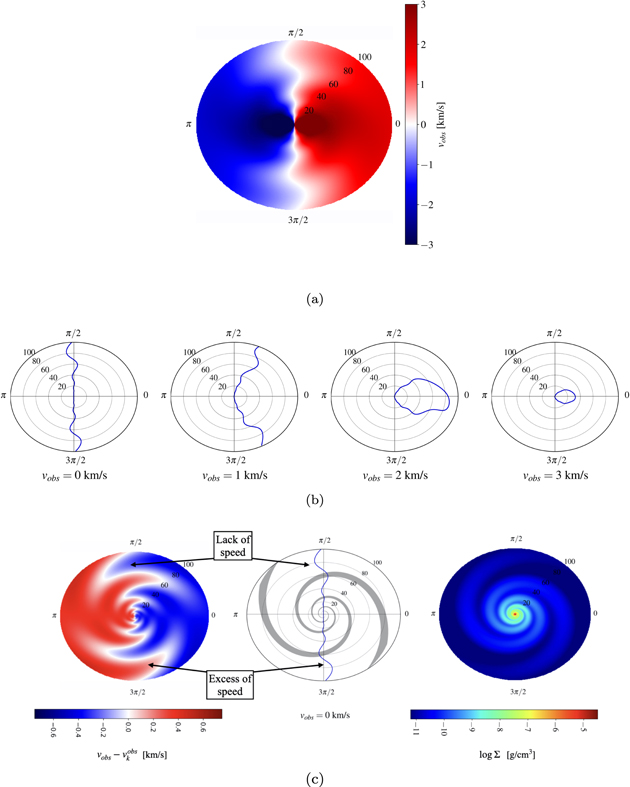
Figure 1. Moment-1 map (a) and channel maps (b) for a self-gravitating accretion disk seen with an inclination angle of π/6 and with a systemic velocity vsyst = 0. (c) Left panel: projected map of the velocity perturbation, after subtraction of the Keplerian field. A system of interlocking fingers is clearly visible, as already noted by H20. Central panel: the vobs = 0 contour (blue line) overlaid with the spiral shape (gray line). The deviations from the Keplerian channel (that is simply a straight line) perfectly match with the spiral pattern. Right panel: surface density of the disk. The parameters of the disk are the following: rin = 1 au, rout = 100 au, M⋆ = 1 M⊙, Md = 0.3M⋆, p = −1, β = 5, αp = 15°, and m = 2.
Download figure:
Standard image High-resolution imageWe want to underline that in this work we are only considering the projection of the velocity field along the line of sight, without making any assumptions about the gas emission processes. In order to convert velocities to fluxes, it is necessary to include the physics of the gas, specifying the selected tracer and the emission lines observed and considering also the effect of the beam size and the eventual presence of observational noise. To do so, we should use radiative transfer codes, as done in H20.
5. Discussion and Conclusions
5.1. Shape of the Wiggle
So far, we have seen that deviations from the Keplerian behavior are visible in every channel map; however, we now focus on the central velocity channel that, in a case where vsyst = 0, corresponds to vobs = 0. As far as the Keplerian case is concerned, the central channel is simply a straight line, because the radial velocity is zero. In the spiral-perturbed case, the central channel shows oscillation around the Keplerian behavior (i.e., the wiggle): this happens because the spiral wave perturbs both the azimuthal and the radial component. The amplitude and the radial frequency of the wiggle depend on the strength of the spiral wave (which is related to the cooling factor β ), the opening angle αp , and the number of arms m (Figure 3), and on the structure of the underlying disk, in particular its mass.
It is possible to quantify the amplitude of the VP considering the integrated geometrical distance between the perturbed and the unperturbed channel. Mathematically, a channel map Cv
is a 2D curve defined parametrically from a one-dimensional interval  to a two-dimensional space
  . In our case, the two-dimensional space is the cylindrical space (r, ϕ) and the interval
  depends on the parameterization we choose: for simplicity, we take
 ![${ \mathcal I }=[0,1]$](https://content.cld.iop.org/journals/2041-8205/920/2/L41/revision1/apjlac2df6ieqn13.gif) . For a given channel velocity v, we call the Keplerian channel map Cv
k
and the perturbed one Cv
p
: mathematically speaking, the two channel maps can be written parametrically as
. For a given channel velocity v, we call the Keplerian channel map Cv
k
and the perturbed one Cv
p
: mathematically speaking, the two channel maps can be written parametrically as

where s is a parameter in the interval  , in our case s ∈ [0, 1]. The amplitude of the perturbation is then computed as
which is the length of the curve  . Panel (a) of Figure 2 schematically shows the quantities involved in Equation (25). The amplitude is determined by both the cooling factor and the disk mass: a smaller β generates a bigger deviation from the Keplerian case, because the amplitude of the density perturbations is inversely proportional to β (Equation (11)). In panel (b) of Figure 2 we show the amplitude of the wiggle (vobs = 0) as a function of the cooling parameter β: it is possible to describe the relation between
  and β as a power law, with an index of −1/2, and this can be easily seen from Equation (22). The role of the cooling factor acts as the planet mass in the case of planetary kinks: indeed, the amplitude of the kink is determined by the mass of the embedded protoplanet, and it follows the relation
  (Bollati et al. 2021). In addition, the amplitude of the wiggle is also determined by the disk mass: in particular, it affects the perturbed velocities because it is related to the sound speed. Indeed, with the hypothesis of Q ≃ 1 we get cs
= uk
H/r ≃ uk
Md
/M⋆. The disk mass is directly proportional to the sound speed, and then bigger cs
means faster propagation of density waves. Panel (c) of Figure 2 shows how the amplitude of the wiggle depends on the disk mass. The trend is easily explained by looking at the equation of the VPs (22): in the radial perturbation, the disk mass appears with a quadratic dependence, while in the azimuthal one, it appears linearly. The amplitude of the channel (25) is proportional to the root sum of squares, thus
(Bollati et al. 2021). In addition, the amplitude of the wiggle is also determined by the disk mass: in particular, it affects the perturbed velocities because it is related to the sound speed. Indeed, with the hypothesis of Q ≃ 1 we get cs
= uk
H/r ≃ uk
Md
/M⋆. The disk mass is directly proportional to the sound speed, and then bigger cs
means faster propagation of density waves. Panel (c) of Figure 2 shows how the amplitude of the wiggle depends on the disk mass. The trend is easily explained by looking at the equation of the VPs (22): in the radial perturbation, the disk mass appears with a quadratic dependence, while in the azimuthal one, it appears linearly. The amplitude of the channel (25) is proportional to the root sum of squares, thus  , where c1 and c2 are two constants that depend on the other parameters, such as the cooling.
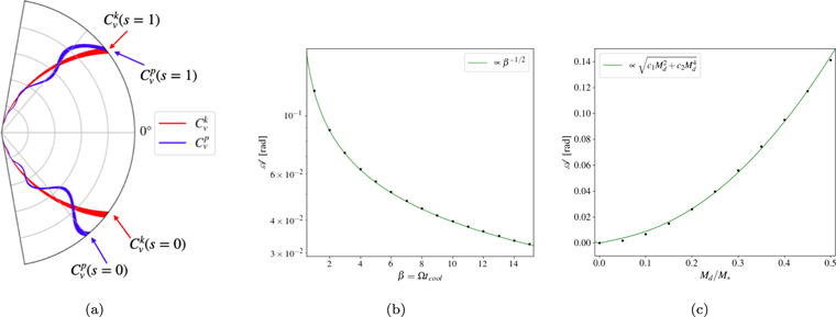
Figure 2. Schematic view of how the amplitude of the wiggle is computed (a): the red line is the Keplerian channel map, while the blue line is the perturbed one. The amplitude of the perturbation is computed using Equation (25). Amplitude of the central channel as a function (b) of the cooling parameter β for a disk mass Md /M⋆ = 0.3 and (c) of the mass of the disk for a cooling parameter β = 5. The black dots are the results of the analytical model so far described.
Download figure:
Standard image High-resolution imageThanks to the analytical expression for the VPs, we can infer in what regimes the radial or azimuthal perturbation dominates the wiggle. As we have already noted, for larger Md /M⋆ the radial perturbation dominates. This is a crucial point because a perturbation of the channel vobs = vsyst is visible only if there is a radial perturbation: indeed, as in the Keplerian case, if the velocity is purely azimuthal, the central channel is a straight line.
Unfortunately, the mass of the disk and the cooling β are degenerate parameters when we consider the shape of the wiggle: as a matter of fact, they both contribute to its amplitude. Is it possible to break the degeneracy? This can be done if an independent method to measure Md is available. For example, using again the gas kinematics, one could measure deviations from Keplerianity in the azimuthally averaged rotation curve, and compute the mass of the disk through Equation (2), breaking the degeneracy. Veronesi et al. (2021) did it for the system Elias 2–27, giving a dynamical estimate of the mass of the disk Md ≃ 0.08 M⊙ ≃ 0.17 M⋆. Conversely, when an approach like this is not possible, we can give a rough estimate of the disk mass through dust emission. Indeed, from dust thermal emission it is possible to measure the dust mass of the disk and then, assuming a dust-to-gas ratio, we also can estimate the total mass of the disk.
Interestingly, if we look at the perturbed velocity field, there could also be a purely kinematical way to break the degeneracy between disk mass and cooling. Indeed, if we write the observed velocity field for ϕ = π/2 (semiminor axis of the disk) we get

where f1 is a known function of radius; conversely, for ϕ = 0 (semimajor axis of the disk) we get
where f2 is a known function of the radius. Since the perturbed velocities scale differently with disk mass, if we could measure accurately the ratio of the two components of the perturbed velocity, we could in principle directly obtain a measurement of the disk mass. However, we note that it is challenging to extract this information from an actual observation.
Breaking the degeneracy allows us to constrain the cooling parameter β, which gives important information about the physical processes that are happening in the protoplanetary environment, and on the tendency of the disk to fragment into bound clumps.
So far we have described what determines the amplitude of the wiggle: as far as its frequency is concerned, it is determined by the pitch angle and by the number of spiral arms. In Figure 3 we show the shape of the wiggle for different values of αp and m. We clearly see that the frequency of the wiggle is bigger when decreasing αp and increasing m.
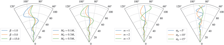
Figure 3. Shape of the wiggle varying (from left to right) the cooling factor β, the mass of the disk Md , the pitch angle αp in degrees, and the azimuthal wavenumber m. The reference disk parameters are rin = 1 au, rout = 50 au, M⋆ = 1 M⊙, Md = 0.3 M⋆, p = − 1, β = 5, αp = 15°, and m = 2.
Download figure:
Standard image High-resolution image5.2. Limitations
As can be seen in Figure 3, the number of spiral arms slightly influences the amplitude of the wiggle: all the calculations have been made under the WKB assumption that requires m/rk << 1. Thus, for high m, this assumption is not valid anymore: in fact, we are not considering the relations between the number of spiral arms and the mass of the disk, or its thickness; the only way to take into account these nonlinear effects is by means of numerical simulations (Terry et al. 2021). This argument is better understood when looking at Equation (3): in the tight winding approximation (WKB), m does not enter explicitly in the dispersion relation (except in the Doppler-shifted frequency), thus both axisymmetric (m = 0) and nonaxisymmetric (m ≠ 0) perturbations have the same instability threshold. However, it is well known (Ostriker & Peebles 1973) that massive disks are subject to large-scale nonaxisymmetric instabilities even though Q > 1. Indeed, a local dispersion relation can also be obtained in the case of open spiral structures (Lau & Bertin 1978): it is a cubic rather than quadratic expression in k and depends on a new dimensionless parameter

Being a function of m and Md
, the  criterion takes into account how massive the disk is and the number of spiral arms: massive disks are prone to exhibit low-m modes instability. Indeed, there is a link between the number of spiral arms and the mass of the disk (Dipierro et al. 2014).
Another important point to stress is that we constructed a 2D model of the disk, neglecting its height. Thus, we are basically considering only what happens in the disk midplane. The main effect of the disk thickness is to "dilute" the gravity field, and this can be incorporated into the quadratic dispersion relation

In this case, the stability criterion only changes slightly, becoming Q ≳ 0.647 (Kratter & Lodato 2016). Observationally speaking, the disk thickness is important when we take into account the molecular line emission of CO isotopologues. As a matter of fact, 12CO, which is the most abundant isotopologue, is not a good tracer of the disk midplane, because it becomes optically thick at the disk surface. On the contrary, other less abundant CO isotopologues such as 13CO or C18O have more optically thin lines and as a consequence they trace better the disk midplane (Miotello et al. 2014).
In addition, our analysis takes into account a single spiral mode m, while it is well known that for small disk-to-star mass ratio, there could be a superposition of modes. However, this is not an actual problem: indeed, we know that after filtering out through the ALMA response (which we do not do in this paper), as shown in Dipierro et al. (2014), only the dominant mode appears. This makes our single-mode analysis still valid.
5.3. Constraining the Cooling Factor—Mock Test
So far, we have seen that the cooling factor deeply influences the shape of the channel maps. Thanks to this property, we propose a method with which we can constrain effectively the cooling factor of observed systems. In order to verify the accuracy of the calculations we have made, we apply the method just described to a numerical simulation. We perform a smoothed particles hydrodynamics (SPH) simulation using the code PHANTOM (Price et al. 2018b). This code is widely used in the astrophysical community to study gas and dust dynamics in accretion disks (Toci et al. 2020a; Ragusa et al. 2020; Veronesi et al. 2020); in this work, we used the so-called "one fluid" method, and we simulated a gas-only disk, neglecting the dust component. The initial conditions of the disk are rin = 1 au, rout = 50 au, Σ ∝ r−1, Md = 0.5, and M⋆, M⋆ = 1 M⊙. The cooling factor β has been set to β = 8 and the two parameters that control the artificial viscosity to αAV = 0.1, βAV = 0.2, in order to reduce as much as possible the effects of artificial dissipation (Lodato & Rice 2004). The initial sound speed profile follows a simple power law cs ∝ r−0.25. However, this profile is rapidly modified by the cooling. For this simulation, we used N = 5 × 10⁵ particles of gas. The simulation shows a predominance of the m = 2 azimuthal mode, and the computed pitch angle is αp ∼ 13°.
We now constrain the cooling factor using the method described previously, and make a comparison with the actual value set in the simulation. First of all we compute the rotation curve, azimuthally averaging uϕ
(r, ϕ). Then, we find the value of the disk mass that best describes the curve using Equation (2): the best value corresponds to Md
= 0.5M⋆, as expected. We have broken the degeneracy between the mass and the cooling: thus, we are now able to constrain the cooling β through the wiggle amplitude. Figure 4 shows the central channel of the projected velocity field of the simulation compared with the one from the analytical model, for different spiral angles: as expected, a wiggle is present. The amplitude of the simulated wiggle
6
is  . The amplitude of the wiggle as a function of the cooling factor, for the parameters previously reported, is described by
  , where
  . The estimated cooling factor is then
  , which is in good agreement with the real value β = 8. The overestimated value of β can actually be interpreted by the lack of viscosity in our analytical model. Indeed, because of its dissipative nature, we expect it to damp GI-driven perturbations, resulting in a less pronounced wiggle. This behavior is visible in the comparison with the numerical simulations, hence the simulated perturbation appears less wide than the analytical one.
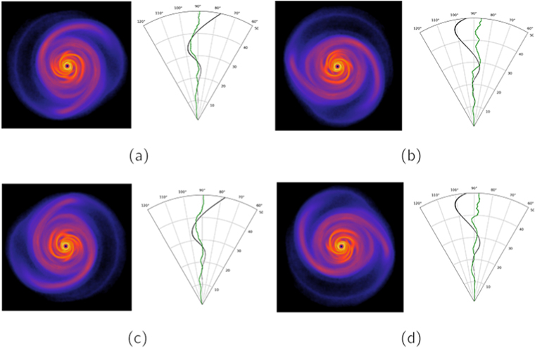
Figure 4. Comparison between analytical (black line) and numerical (green line) perturbation for different viewing angles of the simulated GI disk. Each picture is rotated along the z-axis of an angle of π/2.
Download figure:
Standard image High-resolution image
Figure 4 shows a comparison between the analytical and the numerical wiggle, for different viewing angles of the spiral structure (the observer is assumed to be along a vertical line at the bottom of the images). There is a very good agreement in panels (a) and (c) for which the line of sight intercepts the largest extent of the spiral, while the perturbation is overestimated in panels (b) and (d) in which the prominent spiral structure lies on a line perpendicular to the line of sight. For the former case, the agreement between our model and the simulation is remarkable. For the two other orientations, while there is good agreement in the inner disk (where the perturbation is however smaller), our model overestimates the perturbation in the outer disk, where in the simulation the spiral structure vanishes. This suggests that in actual observations, our analysis is most reliable when a density spiral (for example traced by the dust continuum) is also visible superimposed to the kinematical wiggle.
5.4. Conclusions
In this work we have analytically studied the velocity perturbations in a self-gravitating disk caused by the presence of a spiral density wave in the WKB regime. We then applied this result to obtain the projected velocity field (moment-1 equivalent) and the channel maps, studying their deviations from the Keplerian case. We found what H20 have already seen from numerical simulations, that deviations from Keplerian rotation are a global phenomenon, resulting in velocity "kinks" across the entire radial and azimuthal extent of the disk. The kinematics deviations, called GI wiggles, depend on the structure of the spiral density wave, namely, its amplitude (connected to the cooling and to the disk mass) and its radial frequency (connected to the pitch angle and to the azimuthal wavenumber).
Pinte et al. (2020) found nine deviations from Keplerian rotation pattern in the DSHARP circumstellar disks: three of them, Elias 2–27 (Pérez et al. 2016; Paneque-Carreño et al. 2021), IM Lup, and WaOph6 show also spiral structures in the millimetric continuum emission. These three systems are believed to be self-gravitating (Huang et al. 2018), thus their deviations from Keplerian rotation may be interpreted as wiggles. In addition, Veronesi et al. (2021) have shown that the rotation curve of Elias 2–27 is better described adding the contribution of the disk gravitational potential, meaning that the effects of disk self-gravity are not negligible.
Higher-resolution observations of systems like those will make it possible to investigate the cooling of protoplanetary disks: indeed, the degeneracy between mass and cooling can be broken by means of the rotation curve, and thus the cooling parameter β can be constrained effectively through the wiggle's amplitude, as we have shown in Section 5.3. Knowing more about the cooling will give us insights about the gravitational instability process.
The authors thank the anonymous referee for insightful comments and suggestions, and Richard Booth, Cathie Clarke, and Pietro Curone for useful discussions. This project has received funding from the European Union's Horizon 2020 research and innovation program under the Marie Skłodowska-Curie grant agreement No. 823823 (DUSTBUSTERS RISE project). B.V. acknowledges funding from the ERC CoG project PODCAST No 864965.
Facility: SPLASH: an interactive visualization tool for SPH data (Price 2007).
Footnotes
- 6
Here, we refer to panel (a) of Figure 4.