


Abstract
In 2019, Sgr A*—the supermassive black hole in the Galactic Center—underwent unprecedented flaring activity in the near-infrared (NIR), brightening by up to a factor of 100 compared to quiescent values. Here we report Atacama Large Millimeter/submillimeter Array (ALMA) observations of Sgr A*'s continuum variability at 1.3 mm (230 GHz)—a tracer of the accretion rate–conducted one month after the brightest detected NIR flare and in the middle of the flaring activity of 2019. We develop an innovative light-curve extraction technique which (together with ALMA's excellent sensitivity) allows us to obtain light curves that are simultaneously of high time resolution (2 s) and high signal-to-noise ratio (∼500). We construct an accurate intrinsic structure function of the Sgr A* submm variability, improving on previous studies by about two orders of magnitude in timescale and one order of magnitude in sensitivity. We compare the 2019 June variability behavior with that of 2001–2017 and suggest that the most likely cause of the bright NIR flares is magnetic reconnection.
Export citation and abstract BibTeX RIS
1. Introduction
Sagittarius A* (Sgr A*) is a non-thermal and variable source associated with a black hole at the center of our Galaxy. It has been regularly monitored for over 25 yr and shows variability and flaring activity on scales between minutes to hours across the electromagnetic spectrum–radio, millimeter (mm), submillimeter (submm), near-infrared (NIR), and X-ray (Dexter et al. 2014; Bower et al. 2015; Witzel et al. 2021). The NIR activity is particularly well studied due to regular monitoring of stellar orbits around the Galactic Center (Genzel et al. 2010; Morris et al. 2012; Witzel et al. 2018; Gravity Collaboration et al. 2020).
On 2019 May 13, Do et al. (2019) detected an unprecedentedly bright NIR flare, during which the flux reached at least 100 times the typical Sgr A*'s quiescent value (twice as bright as the strongest flare previously recorded). Sgr A* continued producing bright flares until (at least) the end of the year. Do et al. (2019) and Gravity Collaboration et al. (2020) suggested that the flares might be connected to the recent passage of the S0-2(S2) star. Murchikova (2021) argued against the S0-2 connection and showed that the time of the flaring activity is consistent with the nearly simultaneous arrival of material shed by G1 and G2 objects (formerly known as clouds) near their pericenter passage. In either scenario, the increased mass accretion rate stimulates production of bright NIR flares.
The submillimeter flux density of Sgr A* is generally believed to be a tracer of the accretion rate, as it is dominated by a population of thermal electrons (e.g., Yuan & Narayan 2014; Bower et al. 2019). If the flaring activity of 2019 correlates with an increased accretion rate, it should have been accompanied by a higher submm flux. Here we report 500 minutes of observations of Sgr A*'s continuum variability at 230 GHz (1.3 mm), spread over five epochs in 2019 June, which were conducted by the Atacama Large Millimeter/submillimeter Array (ALMA).
For this work, we develop a light-curve extraction algorithm based on the model fitting in the (u,v)-plane. It allows us to achieve 2 s time resolution with a signal-to-noise ratio of about 500 (surpassing the existing literature by at least an order of magnitude).
The paper is organized as follows. In Section 2 we present the details of the observations and the light-curve extraction algorithm. In Section 3 we discuss the properties of the light curves we obtained. In Section 4 we compare our results with the variability studies in the literature. We present conclusions in Section 5.
2. Observations and Data Analysis
Our data were obtained in ALMA Cycle 6 with 51 antennas in the C43-9/10 configuration for project 2018.1.01124.S (PI: Murchikova). Seven observations were conducted between 2019 June 12 and June 21 (Table 1). Observations span frequencies between 228.55 and 233.8 GHz, with four 1.875 GHz spectral windows centered on 229.50, 230.95, 231.90, and 232.85 GHz. The central frequency is 231.2 GHz. The achieved resolution is 0 025. The achieved sensitivity is 0.04 mJy over a 200 km s−1 frequency range. The bandpass calibrator, phase calibrator, and check source are J1924–2914, J1744–3116, and J1752–2956, respectively. For the data reduction, data processing, and light-curve subtraction we used the Common Astronomy Software Applications package (CASA), version 5.7. For calibration and data reduction we used the script provided by the North American ALMA Science Center at the National Radio Astronomy Observatory.
Table 1. The 2019 June Observations
| Obs | Date | Start time | End time | Mean | σobs |
|---|---|---|---|---|---|
| id | UTC | UTC | UTC | Jy | mJy |
| 0 | 2019 Jun 12 | 03:36:36.5 | 04:51:03.9 | 4.62 | 9.5 |
| 1 | 2019 Jun 13 | 07:11:55.6 | 08:25:06.7 | 3.14 | 6.9 |
| 2 | 2019 Jun 14 | 06:25:00.6 | 07:38:28.5 | 3.33 | 15.5 |
| 3 | 2019 Jun 20 | 07:15:22.9 | 08:28:25.0 | 3.58 | 2.8 |
| 4 | 2019 Jun 21 | 02:35:05.7 | 03:49:47.6 | 4.03 | 4.0 |
| 5 | 2019 Jun 21 | 04:17:04.5 | 05:31:14.7 | 3.70 | 4.6 |
| 6 | 2019 Jun 21 | 05:58:35.3 | 07:12:23.3 | 3.81 | 4.3 |
Note. The seven ALMA observations of the Sgr A* conducted in 2019 June. Observation number, epoch, average continuum flux, and observation uncertainty derived from data are given for each observation.
Download table as: ASCIITypeset image
We phase-self-calibrated each observation independently using line-free channels. As a model of the source for each iteration of self-calibration we fitted a narrow Gaussian to the location of the black hole in the (u,v)-plane using the CASA task uvmodelfit.
We develop a new algorithm for extracting variability information. After phase-self-calibration we collapse the data cube along the frequency axis using all of the line-free channels. We then split the (u,v)-data time stamp by time stamp and find the best-fit point-source model. 3 This allows us to extract the light curves at the telescope's data output cadence, which is 2 s for these observations. The excellent ALMA sensitivity allows us to achieve a signal-to-noise ratio of about 500 per each data point. We extract 1359 data points for each 74 minute observation (Figure 1). As (u,v)-model fitting occasionally fails on the scale of a few percent, we remove points that are outstanding more than 1%–1.5% from the average of their 10 closest neighbors. The total number of removed points is between 54 and 140 per observation, i.e., 4%–10%.

Figure 1. Variation of Sgr A* continuum flux at 230 GHz with time, i.e., light curves for our seven observations in ALMA Cycle 6. The observations are taken in 2019 June, one month after the extraordinary flare of Do et al. (2019) and in the midst of the flaring activity of 2019. We averaged the data between the frequencies of 228.55 and 233.8 GHz. The exact central frequency is 231.2 GHz. The start time of the observation is marked in the bottom right corner of each panel. Each point plotted represents a 2 s integration. Gaps in the light curves are due to observations of the calibrators. The three consecutive observations are plotted together on the bottom panel. Due to weather conditions, observational sensitivity varies from epoch to epoch. It is not uncommon to see occasional spurious features like those in the 2019 Jun 12 data set, mostly at the ends of scans, which are sometimes related to short-term issues with a subset of antennas.
Download figure:
Standard image High-resolution imageThe emission from the Galactic Center minispiral is largely resolved out in our observations. Its total integrated emission across the whole field of view is about 0.25 Jy. This extended emission has a different (u,v)-signature compared to the central point source. It contributes to the uncertainty of the model fit on the scale of 0.4 mJy, which is smaller than our observational uncertainties. In cases of low-resolution data and/or to improve on the precision of the light curves, it is important to subtract the (u,v)-signature of the minispiral before extracting light curves.
Typically, variability studies using ALMA data employ imaging. Reliable imaging requires binning data into about 1–1.5 minutes blocks. Consequently, the time resolution of Sgr A* light curves obtained with ALMA in the literature are about 30–50 times lower than ours. The highest-cadence light curves published in the literature are from the Submillimeter Array (SMA) and have a time resolution of 15 s. However, on average, SMA's signal-to-noise ratio is considerably lower than ALMA's. The latter is also the case for other telescopes referenced here.
Our algorithm utilizes the highest cadence permitted by the telescope and all available (u,v)-data. To avoid light-curve contamination with extended emission we use a (u,v)-model fitting. We therefore avoid unnecessary imaging of data on short time intervals which tends to be affected by artifacts and results in higher uncertainties for light-curve points. The downside of our algorithm is that it is computationally expensive.
3. Results and Intrinsic Structure Function
Figure 1 shows the 230 GHz variability of Sgr A* in 2019 June. The average flux across our observations is 3.74 Jy. The minimum and maximum across all observations, calculated as an average of 10 neighboring points, are 3.04 and 4.77 Jy.
To quantify variability properties, we construct the structure function (or a square root of variance)
where τ is the time lag, F(t) is the flux at time t, Nτ is the number of pairs of points separated by the time interval τ in the data, and the summation runs over all such pairs.
At small timescales, the structure function computed this way tends to be dominated by observational uncertainties. It is easily seen from flattening of the structure functions found in the literature (e.g., Dexter et al. 2014; Iwata et al. 2020; Witzel et al. 2021) at the level of an average observational uncertainty.
Let us introduce the intrinsic
structure function
 , which can be computed from observed structure function by removing the contribution of observational uncertainties
Here SFobs is a structure function of each individual observation,  is a pair count within each individual observation, and the summation runs over independent observations. We treat the consecutive observations 4, 5, and 6 as one observation.
To derive Equation (2) we notice that in the presence of observational noise the observed flux F(t) at time t can be decomposed into the sum of the true flux  and a contribution of observational noise δ
f(t) such that
and a contribution of observational noise δ
f(t) such that  Then the structure function obtained using the data from each observation SFobs(τ) can be rewritten as (see also Simonetti et al. 1985)

where  is the intrinsic structure function and
  is the mean-square root observational uncertainty. The Equation (5) can be recast as Equation (2) for multiple observations.
The derivation holds precisely only for a large sample size, as it relies on the fact that an expectation value of two independent distributions  and δ
f is the product of expectation values for these distributions individually:
and δ
f is the product of expectation values for these distributions individually:  if 〈δ
f〉 = 0. In case of a small sample size, as is the case of all variability studies so far, the observational uncertainties cannot be subtracted completely.
if 〈δ
f〉 = 0. In case of a small sample size, as is the case of all variability studies so far, the observational uncertainties cannot be subtracted completely.
The resulting structure function is plotted in Figure 2. We find that the structure function for τ < 25 minutes scales approximately as τ0.8. At τ ∼ 2 s the imperfection of determining σobs and lack of statistics (which is still the case even in this comparatively large sample) influences the result. At longer timescales τ ≥ 25 minutes the size of our sample begins to influence the results, as the number of independent (F(t + τ), F(t)) pairs decreases, and the sample is dominated by the three consecutive 2019 June 21, observations. We still present the structure function at larger timescales in Figure 2.
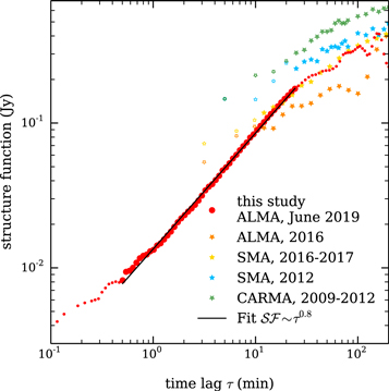
Figure 2. Comparison of intrinsic structure functions of Sgr A* variability at 230 GHz. The 2019 June  is in red. Large circles represent statistically reliable time range 30 s < τ < 25 minutes. The black line is the power-law fit. Small circles represent low statistics points at τ > 25 minutes and τ < 30 s where the noise subtraction was less reliable. The intrinsic structure functions obtained with data from ALMA, SMA, and CARMA at various epochs is presented with stars. Empty stars represent the points where the observational uncertainties could not be reliably subtracted. ALMA data from 2016 (orange) and SMA data from 2016–2017 (yellow) are from Witzel et al. (2021). We removed their only 2015 data set due to its high level of noise. SMA data from 2012 (blue) and CARMA data from 2009–2012 (green) are from Dexter et al. (2014). The plotted intrinsic structure functions are obtained by subtracting known uncertainties. The remaining uncertainties are primarily statistical, i.e., due to the finite size of the data set and an accuracy of determining the observational uncertainties. The latter is dominating the uncertainties on our combined
  , we estimate
  Jy, where 〈σobs〉 is the mean observational uncertainty.
Download figure:
Standard image High-resolution image4. Discussion and Comparison
We compare our results with previous studies of Sgr A* variability at 230 GHz. Witzel et al. (2021) use the 3000 minutes of data observed in 2015–2017 and include the data sample of Iwata et al. (2020). Bower et al. (2015) use the data observed in 2013–2014. Dexter et al. (2014) use the data observed in 2001–2012. The latter study is over the largest time span, however, the data are sparse and irregularly sampled, and consist of a total of 1044 data points.
Since Sgr A* is a highly variable source and in the view of the sparsity of observations there is little value in comparing the minimum and maximum fluxes encountered during the observations. These values are highly volatile and they are additionally affected by the absolute flux-level calibrations. 4 Instead, we compare global statistical measures such as mean values and structure function values.
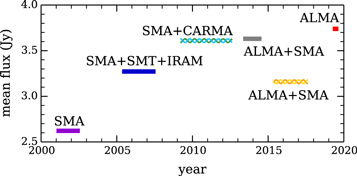
The comparison of mean flux densities over the last 20 yr is presented in Figure 3. In 2019 June we obtained a mean flux value of 3.74 Jy. This is 20% higher than in the epoch directly preceding it (Witzel et al. 2021). It is, however, only 3% higher than in 2009–2012 and in 2013–2014 (Dexter et al. 2014; Bower et al. 2015). The submm flux is dominated by a population of thermal electrons and is expected to vary together with the mean accretion rate (Yuan & Narayan 2014; Bower et al. 2019). There is a slow variability of the mean Sgr A* flux in the submm on the scale of ∼10 yr (Figure 3) which is similar to the expected global mass accretion variability (Ressler et al. 2020). Therefore, we deduce that the mean accretion rate in 2019 June is about 20% higher than in 2015–2017 and about the same as in 2009–2012.
Figure 3. Comparison of mean flux densities of Sgr A* at 230 GHz. Red: 2019 June data (red). Intertwined orange and yellow: 2015–2017 data from Witzel et al. (2021). Grey: 2013–2014 data from Bower et al. (2015). Intertwined blue and green: 2019–2012 data from Dexter et al. (2014). Dark blue: combined 2005–2007 data from Marrone et al. (2008) and Yusef-Zadeh et al. (2009). Violet: 2001–2002 data from Zhao et al. (2003). The telescopes that obtained the data are listed next to the mean flux density. We combine the data sets such that there are about 10 epochs in each. The typical standard deviation is ∼0.5 Jy. To calculate the mean of the data from Bower et al. (2015) we average their eight ALMA data points and the 16 SMA data points at 226.85 GHz.
Download figure:
Standard image High-resolution image
The comparison of intrinsic structure functions of Sgr A*  defined in Equation (2) with the one derived in this work is shown in Figure 2. We use Dexter et al. (2014) and Witzel et al. (2021) (included with the publications) data to recalculate the corresponding intrinsic structure functions at earlier epochs. Due to low statistics and the fact that at the shortest timescales the
  the earlier intrinsic structure functions are still affected by observational uncertainties at timescales < 10 minutes. No variability comparison is possible with Bower et al.'s (2015) 2013–2014 data, as they have only one epoch of monitoring.
The slope of the 2019 structure function of 0.8 is consistent with red noise (Emmanoulopoulos et al. 2010) and 1σ consistent with the power spectrum determined by Witzel et al. (2021). The high signal-to-noise ratio of the high-cadence observations of 2019 allows us to demonstrate for the first time that the red noise characteristics of the mm-variability of Sgr A* continue down to a time lag of 30 s. The red noise behavior seems to be intrinsic to the source. The overall level of Sgr A* variability in 2019 June seems to be the same or somewhat higher than that of 2016–2017 and somewhat lower than that of 2009–2012. An accurate comparison of the variabilities is complicated by the systematic differences among the derived historic structure functions, some of which may be due to higher uncertainties in observations in 2000 s.
5. Conclusion
We present ALMA observations of Sgr A* variability at 230 GHz in 2019 June (Figure 1). ALMA's excellent sensitivity together with a new light-curve extraction algorithm developed for this work allows us to achieve a combination of high cadence (2 s) and high signal-to-noise ratio (∼500), which surpasses light curves available in the literature by a factor of 10–100.
We construct an intrinsic structure function of Sgr A* variability at 230 GHz by subtracting the contribution of observational uncertainties as described in Section 3, with the result shown in Figure 2. We push the range of validity of the structure function by about two orders of magnitude toward shorter timescales. We find that it can be approximated by the power-law  on timescales 30 s ≤ τ ≤ 25 minutes.
Our observations are taken one month after the brightest NIR flare of Do et al. (2019) and in the midst of the NIR flaring activity of 2019. Using the connection between the submm flux of Sgr A* and the accretion rate (Yuan & Narayan 2014; Bower et al. 2019), we conclude that the flaring activity of 2019 coincides with the period of elevated accretion rate onto the black hole as compared to the epoch directly preceding it (Witzel et al. 2021), in agreement with the calculation of Murchikova (2021).
We find that the elevated accretion rate was not the trigger of the bright NIR flares observed in 2019 (Do et al. 2019; Gravity Collaboration et al. 2020). An almost identical mean submm continuum flux and consequently the identical mean accretion rate was observed between 2009 and 2014 (Dexter et al. 2014; Bower et al. 2015) when no bright flaring activity was reported (Figure 3). Bright NIR flares in general do not get brighter with increased accretion rate, hence their relation to the accretion rate, if any, must be indirect.
Among the physical mechanisms proposed as possible origins of the NIR flares such as the population of non-thermal electrons, magnetic reconnection, and shocks (Yuan et al. 2003; Dodds-Eden et al. 2010; Yusef-Zadeh et al. 2012; Ponti et al. 2017), the one most independent from the accretion rate is magnetic reconnection (Ripperda et al. 2020, 2021). We therefore suggest that the brightest NIR flares of Sgr A* are likely caused by magnetic reconnection. We stress that this statement is related only to the brightest among the NIR flares of Sgr A*. The full phenomenology of the variability is likely produced by a combination of the mechanisms listed above.
We are grateful to Jason Dexter, Mark Gurwell, Brian Mason, Sasha Philippov, Eduardo Ros, Nadia Zakamska, and the anonymous referee for comments and suggestions. L.M.'s membership at the Institute for Advanced Study is supported by the Corning Glass Works Foundation. A part of this work was performed at the Aspen Center for Physics, which is supported by National Science Foundation grant PHY-1607611. The participation of L.M. at the Aspen Center for Physics was supported by the Simons Foundation.
This Letter makes use of the following ALMA data: ADS/JAO.ALMA#2018.1.01124.S. ALMA is a partnership of ESO (representing its member states), NSF (USA) and NINS (Japan), together with NRC (Canada) and NSC and ASIAA (Taiwan) and KASI (Republic of Korea), in cooperation with the Republic of Chile. The Joint ALMA Observatory is operated by ESO, AUI/NRAO, and NAOJ.
The National Radio Astronomy Observatory is a facility of the National Science Foundation operated under cooperative agreement by Associated Universities, Inc.
Footnotes
- 3
Fitting either a perfect point-source or a Gaussian source with a variable width and position yields essentially identical results. In both cases, the CASA task uvmodelfit successfully finds the location of Sgr A*. This location does not drift within observations.
- 4
Correcting for the uncertainty in the absolute flux-density calibration is very important in computing the Sgr A* structure function on long timescales, particularly those involving approximations between data sets.