


Abstract
In this work we have, for the first time, applied the interpretation of multiple "ghost-fronts" to two synthetic coronal mass ejections (CMEs) propagating within a structured solar wind using the Heliospheric Upwind eXtrapolation time (HUXt) solar wind model. The two CMEs occurred on 2012 June 13–14 showing multiple fronts in images from Solar Terrestrial Relations Observatory Heliospheric Imagers (HIs). The HUXt model is used to simulate the evolution of these CMEs across the inner heliosphere as they interacted with structured ambient solar wind. The simulations reveal that the evolution of CME shape is consistent with observations across a wide range of solar latitudes and that the manifestation of multiple "ghost-fronts" within HIs' field of view is consistent with the positions of the nose and flank of the same CME structure. This provides further confirmation that the angular separation of these features provides information on the longitudinal extent of a CME. For one of the CMEs considered in this study, both simulations and observations show that a concave shape develops within the outer CME front. We conclude that this distortion results from a latitudinal structure in the ambient solar wind speed. The work emphasizes that the shape of the CME cannot be assumed to remain a coherent geometrical shape during its propagation in the heliosphere. Our analysis demonstrates that the presence of "ghost" CME fronts can be used to infer the distortion of CMEs by ambient solar wind structure as a function of both latitude and longitude. This information has the potential to improve the forecasting of space weather events at Earth.
Export citation and abstract BibTeX RIS

Original content from this work may be used under the terms of the Creative Commons Attribution 4.0 licence. Any further distribution of this work must maintain attribution to the author(s) and the title of the work, journal citation and DOI.
1. Introduction
Coronal mass ejections (CMEs) are spectacular eruptions of plasma and magnetic field transferring huge energies from the solar corona into the interplanetary medium. Their interplanetary counterpart (ICMEs) have been recognized as major drivers of severe space weather (Gosling et al. 1991; Zhang et al. 2007; Shen et al. 2017), which can cause geomagnetic storms and trigger a wide array of undesirable consequences, including anomalies in satellite systems, damage to the ground-based electric power grids, and interference with radio communications and satellite navigation systems (Cannon et al. 2013). In addition, space weather poses health hazards for astronauts and passengers and crew in high-altitude aircraft (Lockwood & Hapgood 2007). This potential hazard to modern technological systems and humans (Eastwood et al. 2017) can be mitigated through better forecasting of CMEs at Earth, which in turn relies on an accurate understanding of a CME's evolution through the inner heliosphere (Owens et al. 2020b).
As the heliocentric orbits of the Solar Terrestrial Relations Observatory (STEREO; Kaiser et al. 2008) cause the two spacecraft to separate from the Earth at a rate of around 22 5 per year, the Heliospheric Imagers (HIs; Eyles et al. 2009), part of the Sun–Earth Connection Coronal and Heliospheric Investigation (SECCHI) suite (Howard et al. 2008), provide an unique and invaluable way to study CME propagation and evolution from two vantage points separated from the Sun–Earth line. The HI instruments open up avenues of research into CME properties that have previously been difficult to pursue and have revolutionized our understanding of the evolution of CMEs as they propagate through the inner heliosphere (Harrison et al. 2017; Chi et al. 2018). Because of the wide observation angles and scattering effects, CMEs are often observed as visually intricate structures in HI images (Jones et al. 2020). The complex structure observed in HI images increase the challenge of tracking each CME through the heliosphere, especially for those CMEs observed with multiple fronts. Multiple CME fronts in HI images appear as bifurcating features when tracked with elongation-time maps (Sheeley et al. 1999), which are usually used to determine CME kinematics and predict the arrival time of CMEs in the near-Earth space. If only the outer front of a CME is considered in the elongation-time map, this can introduce significant errors into the predicted arrival time at Earth (Liu et al. 2016). In some multiple-front events, the outer front has been interpreted as a manifestation of a shock, which appeared as a sharp edge ahead of the ejecta part of CMEs, with the inner front corresponding to the front of ejecta (Liu et al. 2010; Maloney & Gallagher 2011; Hess & Zhang 2014). Recently, Scott et al. (2019) proposed a new interpretation of multiple fronts with similar shape arising from the different part of a single three-dimensional (3D) CME feature projected onto a two-dimensional (2D) HI images. They demonstrated that the outer and inner fronts of the CME were consistent with the elongation angle of the flank and and nose of the outer boundary of CME. Interpreting the formation of the multiple CME fronts as different parts of a single 3D CME front could provide useful information about the longitudinal extent and structure of a CME and thus aid accurate forecasting of a CME's arrival at Earth. This assumption was confirmed by Chi et al. (2020), who used the ghost-fronts model to study two CMEs erupted during 2012 June 13–14 and predicted the arrival time of CMEs at Venus and Earth assuming they had propagated through a uniformed background solar wind.
In general, it has been shown that the transit time of CMEs is significantly controlled by ambient solar wind conditions (Case et al. 2008; Temmer et al. 2011; Owens et al. 2020a). CMEs are accelerated or decelerated depending on the relative speed between the CME and the ambient solar wind (Gopalswamy et al. 2001a). Owens et al. (2017) argued that CMEs should not be considered as coherent structures during their propagation in the heliosphere due to the high expansion speeds and the typical CME length scales. The magnetic structure inside a CME is coherent only on small scales (0.06–0.12 au) in longitude (Lugaz et al. 2018). Exploitation of the HI images have provided observational evidence that CMEs can become distorted, if different parts of a CME encounter different velocity regimes within a structured solar wind, or other features such as multiple CMEs or stream interaction regions (Cargill et al. 1994, 1996, 2000; Farrugia et al. 2005; Owens et al. 2006; Savani et al. 2010; Rollett et al. 2014; Wang et al. 2014). Previous methods to interpret CMEs observations and predict their arrival time in near-Earth space have typically assumed a rigid and designated shape for the CME front during its propagation in the heliosphere (Sheeley et al. 1999; Lugaz et al. 2009; Sheeley & Rouillard 2010; Davies et al. 2012). Such assumptions about the shape of CMEs are likely to be too simplistic when significant spatial gradients in the ambient solar wind conditions are present (Lugaz et al. 2009; Barnard et al. 2017). Therefore, it is not possible to improve our current arrival time predictions, without a good understanding of the ambient solar wind conditions and the subsequent evolution of the overall shape of CMEs.
In the current study, an estimate of the ambient solar wind conditions in the heliosphere is obtained by the Heliospheric Upwind eXtrapolation time (HUXt) model (Owens et al. 2020a), which uses for input the MAS magnetohydrodynamic coronal model (Riley et al. 2001) output. HUXt model is a one-dimensional, incompressible, hydrodynamic model that neglects magnetic forces, yet can closely emulate the outputs from more comprehensive 3D MHD solar wind models (e.g., HelioMAS). With HUXt, a CME is input into the simulation domain as a hydrodynamic spherical structure or a sausage shape (the thickness parameter larger than zero), and the CMEs internal magnetic field is neglected. Therefore, it is not suitable to predict the magnetic field inside the ICME. The model is used to simulate the evolution of global structure of real CMEs, for comparison with observations, estimate the elongation angle of CME flank and nose as a function of time from 30 R⊙ out to 1 au, and predict the CMEs arrival time at any target of interest in the heliosphere.
Two CMEs that erupted during 2012 June 13–14 (previously studied by Srivastava et al. 2018; Kilpua et al. 2019; Scolini et al. 2019; and Chi et al. 2020) were selected for their well-defined multiple fronts observed in HI images and the availability of data that enabled them to be tracked continuously from eruption at the solar surface to Earth. In our previous work (Chi et al. 2020), we have confirmed that the outer and inner fronts of this two CMEs as observed in HI images are consistent with the flank and nose of a single CME front when assuming the background solar wind is uniform. The goals of this Letter are: (1) to investigate whether the interpretation of multiple fronts holds when considering the impact of a structured ambient solar wind, and (2) analyze the shape and kinematics evolution of CMEs affected by the ambient solar wind. A combined modeling/observation approach is presented in this work, in which the graduated cylindrical shell (GCS) model (Thernisien et al. 2006, 2009) was fitted to three contemporaneous coronagraph images from STEREO-A, Solar and Heliospheric Observatory (SOHO), and STEREO-B to provide an estimate of the initial velocity, propagation direction and width of the CMEs. The HUXt model was then used to provide a reconstruction of the ambient solar wind speed through which the model CMEs propagate allowing the evolution of CME dynamics to be investigated. A comparison between the simulation results and HI observations of the two CMEs is presented in Section 2. In situ observations of the two CMEs near Venus and Earth are compared directly with the predicted arrival time and are used to validate our assumptions. Section 3 presents a discussion of our findings and conclusions.
2. Inserting and Tracking ICMEs in the Global HUXt Model
The first CME (CME-1) considered in this work was observed by SOHO/LASCO-C2 at 13:25 UT on 2012 June 13 as a partial halo CME. About 23 hr later, SOHO/LASCO-C2 observed another halo CME (CME-2) at 14:12 UT on 2012 June 14. In order to compare the evolution of the CMEs in HI images and the simulation from the HUXt model, the information on the shape, propagating direction and the initial velocity of the CMEs are needed as inputs to the HUXt model in order to launch 3D ejecta into the background solar wind. We emphasize that the term CME in this work refers to both the shock and sheath regions surrounding the ejecta as well as the ejecta itself. The CME model inputs were derived from the GCS model in which contemporaneous observations from the three vantage points (SECCHI/COR2-B, SOHO/LASCO and SECCHI/COR2-A) were used. In order to be consistent with the assumption of an initial spherical CME shape used in the HUXt model, the two CMEs were fitted using the cone model by setting the GCS model parameter half-angular width (angle between two "legs") α = 0° and aspect ratio (κ, i.e., the ratio of the CME size at two orthogonal directions) close to one, based on the study by Palmerio et al. (2019), Temmer & Nitta (2015), and Schmidt et al. (2016). The aspect ratio obtained from GCS model fitting contributes to the half angle values of the two CME events. Figure 1 show the GCS cone fitting (green mesh) overlaid on running difference images produced from observations made by COR2-B, LASCO C3, and COR2-A for CME-1 (top row) and CME-2 (bottom row). For CME-1, GCS fitting yielded a best-fit longitude of −7°, latitude of −23° and a half angle of 453. The initial longitude, latitude, and half angle of CME-2 were found to be −4°, −20° and 537, respectively. Comparison of our fit results with previous work (Srivastava et al. 2018; Kilpua et al. 2019; Scolini et al. 2019; Chi et al. 2020) shows that there is a good agreement in longitude, latitude, and half angle. These three parameters were fixed throughout the propagation. The injection speeds for CME-1 and CME-2 are 647.2 km s−1 and 1096.4 km s−1, respectively. These were derived from the GCS model at the height of CME apex closest to HUXt models inner boundary (30R⊙). Before CMEs enter the model domain, the velocity of CMEs is assumed to remain constant. The established initial parameters of the two CMEs at height around 30R⊙ (the inner boundary of the HUXt model) and the uncertainty of the the CME initial parameters are listed in Table 1.

Figure 1. GCS fitting (green mesh) for each of the CMEs for contemporaneous images from SECCHI/COR2-B, SOHO/LASCO/C3, and SECCHI/COR2-A, from left to right, respectively. The panels show running difference images of CME-1 (top row) between 17:18 and 17:24 UT on 2012 June 13, and CME-2 (bottom row) between 15:39 and 15:42 UT on 2012 June 14.
Download figure:
Standard image High-resolution imageTable 1. CME Input Parameters Specified for the HUXt Model and the HUXt Model Predicted CME Arrival Times at Venus and Earth
| Initial Time | Longitude | Latitude | Half Angle | Height | Initial Speed | Predicted Arrival Time | Predicted Arrival Time |
|---|---|---|---|---|---|---|---|
| (UT) | (°) | (°) | (°) | (R⊙) | (km s−1) | at Venus (UT) | at Earth (UT) |
| CME-1: | |||||||
| 2012/06/13 | −7(±5) | −23(±5) | 45.3(±10) | 29.1(±2) | 647.2(±50) | 2012-06-16 | 2012-06-17 |
| 20:49 | 02:18:00(+3/−3) | 03:13:00(+7/−2) | |||||
| CME-2: | |||||||
| 2012/06/14 | −4(±5) | −20(±5) | 53.7(±10) | 27.7(±2) | 1096.4(±50) | 2012-06-16 | 2012-06-17 |
| 17:29 | 05:20:00(+3/−3) | 03:13:00(+7/−2) | |||||
Download table as: ASCIITypeset image
As discussed in Chi et al. (2020), both CMEs are well observed in the HI-A and HI-B field of views, showing clear multiple fronts. In order to associate the complex features in HI images with the different parts of the CMEs, we investigate the 3D evolution of CMEs as they propagate through the inner heliosphere using the HUXt model. The HUXt model can simulate the global context of CMEs and trace CMEs through the ambient solar wind in the inner heliosphere from 30 R⊙ onward. The global shapes of CMEs were identified by computing the difference between the ambient and CME solutions, where the speed differences are >20 km s−1. The simulated result and the HI-A/B observations of the two CMEs are shown in an animation in the online journal (see Figure 2). Figure 2 contains two snapshots from the movie around the time when HI-A and HI-B both show clear multiple fronts in CME-1 (top row) and CME-2 (bottom row). The left panels present the HUXt model solution, each showing CMEs and the ambient solar wind together with the relative positions of the spacecraft and planets on the ecliptic plane. STEREO-A and STEREO-B were at 117° and −118° longitude in HEEQ coordinates, respectively. Such a spacecraft configuration indicates the STEREO satellites were at the optimum location to study the CME radial evolution along the Sun–Earth line. The boundaries of CME-1 and CME-2 along the latitudinal plane of Earth are shown in yellow and orange, respectively. Based on the shape of CMEs obtained from the HUXt model, we can compute the maximum elongation of the CME seen by HI-A and HI-B (shown as red crosses for CME-1 and red pluses for CME-2). It should be noted that the tangent point of CME boundary in the HI-A/B field of view (FOV) can switch between locations, due to the distortion of CME shape by the ambient solar wind. As shown in the supplementary video, the presence of the fast solar wind at the west flank of the CME-1 can significantly distort the CME outer shape, resulting in this portion of CME moving faster. The tangent point of the CME boundary may correspond to different points along the front during this evolution. That it jumps suddenly between locations in the simulation is a result of the model resolution. The blue diamonds indicate the propagation direction of CME-1 and CME-2, obtained from the GCS model. Here we define the CME flank as the maximum elongation of a CME front viewed from HI-A or HI-B and the nose of the CME as the front of CME along its central propagation longitude. The HUXt model is a 3D simulation model, and so the elongation angle of the CME nose and flank can be computed at any position angle spanned by the CMEs.
Figure 2. The left panels contain a snapshot of the solar wind speed on the equatorial plane as simulated with the HUXt model. The yellow and orange lines mark the boundaries of CME-1 and CME-2, respectively. The gray shaded areas show the fields of view of HI-A and HI-B. The middle and right panels show the observations of the same CME on the meridional plane from HI-A and HI-B. The dashed-green lines mark a 4° position angle band around the solar equatorial plane. The red cross and red plus mark the flanks of the modeled CME-1 and CME-2. The blue diamonds mark the nose of CMEs. The flank and nose of the modeled CME-1 and CME-2 at each 5° position angle are overlain on the HI images. An animation of this figure is available, showing the evolution of the two CMEs boundary by interacting with the ambient solar wind. It covers 25.3 hr starting at 01:29 on 2012 June 14. The realtime duration of the animation is 7 s.
(An animation of this figure is available.)
Download figure:
Video Standard image High-resolution imageThe middle and right panels of Figure 2 show the running difference images from HI-A/B. In order to interpret the multiple fronts of CMEs observed by HIs, we not only focus on the kinematic evolution of CMEs on the ecliptic plane, but also study the evolution of the CME shapes interacting with the background solar wind in the meridional plane. Based on the assumption of the ghost-front model, we obtained the elongation angle of the flank and noses of the two CMEs and overlaid the simulated results on the HI observations with the same symbols. In the FOV of HI-A, there is a good agreement between the overall shape and position of the simulated CME-1 flank and nose and the multiple fronts observed within HI images of CME-1. In the FOV of HI-B, there are some differences between the simulated front and the observations. The proposed reason for the discrepancy between the predictions and the observations is that our model setup has not accounted for any preceding CMEs in the ambient solar wind. As studied by Kilpua et al. (2019), a preceding CME was captured by COR2-A/B, 19 hr ahead of CME-1, which may alter the conditions in the heliosphere and affect the simulated result. As the evolution of CMEs is associated with the force balance between the CME internal magnetic pressure from the magnetic field and external dynamic pressure at their interaction surface with the ambient solar wind (Scolini et al. 2019), the neglect of the internal magnetic field of the CME also plays a role in the evolution of CME shape. The initial spherical CME shape used in the HUXt model may also cause an uncertainty in the projected front, as the true CME shape is more in line with a flux rope or so-called "croissant". It should be noted that the different parts of each CME's outer boundary appear as the leading front in the FOV of HI-A and HI-B. The panels in Figure 2 illustrate the leading front of CME-1 appears asymmetric as seen by the two HIs at different locations. The outer front of CME-1 in HI-B FOV still retains a clearly circular shape, while in the HI-A FOV, the front displays an extended morphology. The simulation results from HUXt model also show that the shape of CME-1 distorts significantly from its originally circular shape (as defined by the input parameters) due to the latitudinal gradient in ambient solar-wind-speed. Due to the impact of the structured ambient solar wind, the spherical CME shape, which was inserted at HUXt model inner boundary, undergoes a continuous deformation, and the CME can rarely present as a true spherical shape in the simulation domain. Savani et al. (2010) argued that observations of a distorted CME geometry were caused by interaction with a bimodal distribution of solar wind speed (see also the review by Manchester et al. 2014), which might also be confirmed by Solar Orbiter observations (Davies et al. 2021). This interpretation is consistent with the solar wind structure obtained from the HUXt model near the east flank of CME-1.
The inner front of CME-1 in the HI-A FOV is consistent with the position of the nose of CME-1 simulated from the HUXt model. Neither observations nor simulations show a clear distortion for the nose of the CME, indicating that the real solar wind speed was uniform with latitude. The CMEs are not behaving as a single coherent entity as they propagate through a range of different ambient solar wind conditions. Even though the flank of CME showing concave shape in the HI FOV, the nose of the CME, which may encounter the Earth, still maintains a convex shape.
The elongation angle of the nose and flank fronts of CME-2, obtained from the HUXt model, are comparable with the inner and outer fronts of the CME observed in HI images shown in the bottom-middle and right panels. It indicates at least for this two-CME event, the multiple fronts within each CME correspond to the flank and nose of a single CME front. We conclude that the ghost-fronts observed in the HI images can be used to infer the longitudinal structure of a CME as suggested by Scott et al. (2019). Given that CME-2 is traveling faster than CME-1, it is expected that the CME-2 will catch up with CME-1 within the inner heliosphere.
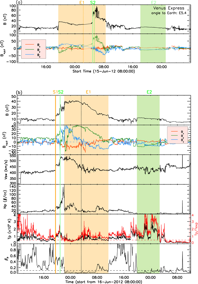
The primary method by which we assess the model forecast validity is by making direct comparison with the in situ observations of the two CMEs. The HUXt model enables prediction of the arrival time and velocity of CMEs at any target of interest in the heliosphere. By simulating a realistic ambient solar wind, a more accurate prediction of the arrival time is expected. The errors of CME arrival time are also estimated by considering uncertainty in CME initial conditions using a 200-member HUXt ensemble runs (Barnard et al. 2020; Owens et al. 2020a). The initial CME parameters are obtained from GCS model fitting with an uncertainty of ±5° in longitude and latitude, ±10° in half angle, ±50 km s−1 in initial velocity, and ±2R⊙ in initial height. The full range of the ensemble CME-1 and CME-2 arrival time distribution spans approximately 6 hr at Venus and 9 hr at Earth. The uncertainties of the CME-1 and CME-2 arrival time are shown in Table 1. During the propagation of the two CMEs, Venus was situated at 0.72 au 54 west of Earth, marked with purple dots in the left panels of Figure 2. Due to the favorable locations of Venus (Venus Express (VEX); Zhang et al. 2006) and Earth (Wind), it is possible to detect the arrival time of the two CMEs at two different locations. Here we use the same explanations of VEX and Wind in situ observations from Chi et al. (2020). The yellow and green regions in Figure 3 indicate the interval of CME-1(E1) and CME-2(E2), respectively. The first detection of CME-1 by VEX was at 19:24 UT on June 15, about 7 hr earlier than the estimated CME-1 arrival time computed by the HUXt model, indicated by the yellow dashed line. The arrival times of the two CMEs at Venus and Earth, estimated by the HUXt model, are presented in Table 1. The arrival time of CME-2 (shock, S2) was recorded at 04:53 UT June 16 at VEX, indicated by the green vertical line at the trailing part of CME-1. The detection time of CME-2 is approximately 1 hr earlier than the predicted arrival time of CME-2 by the HUXt model, indicated by the green dashed line. The in situ observations from VEX suggest that CME-1 and CME-2 have interacted significantly (the shock driven by CME-2 propagating into the CME-1) before they reach the orbit of Venus, which is consistent with the conclusion from Scolini et al. (2019) and Srivastava et al. (2018). The interaction between CMEs can change CME properties, such as their size, velocity (Shen et al. 2012; Lugaz et al. 2017). The discrepancies in arrival times between our HUXt simulation and the in situ observation from VEX may arise from the interaction between the two CMEs. The HUXt simulation indicates that the two CMEs arrived at Venus in close proximity interacting with each other, while at Earth CME-2 has overtaken the front of CME-1. As shown in Figure 3 panel (b), the shock driven by CME-2 (green vertical line, S2) has passed CME-1 (indicated by interval E1). The interval E1 can be identified as a typical ICME interval, based on the criterion of Chi et al. (2016) and Richardson & Cane (2010), with enhanced and smoothly rotating magnetic field, depressed proton temperature, and lower plasma β compared to the ambient solar wind. In the HUXt model, the fronts of the two CMEs merged together. The predicted arrival time of CME-1 and CME-2 are the same at 03:13 UT on June 17, which is about 5 hr later than the shock arrival time of CME-1 and CME-2 observed by the Wind spacecraft. It is noteworthy that, in the current version, the HUXt model is not able to react to possible deflections of CMEs or to simulate elastic or super-elastic collisions between two CMEs (Shen et al. 2012; Schmidt & Cargill 2004) during their propagation, which may cause the observed bias between the simulation and observations.
Figure 3. In situ observations of CME-1 and CME-2 at Venus and Earth. (a) VEX magnetic field strength and the x, y, and z components in VSO coordinates, (b) Wind in situ magnetic (x, y, and z components in GSE coordinates) and plasma data. The yellow and green shaded regions indicate the intervals of CME-1 and CME-2. The solid yellow and green vertical lines indicate the arrival of the shock driven by CME-1 and CME-2, respectively. The expected arrival times of CME-1 and CME-2 are indicated by vertical dashed lines (CME-1:yellow, CME-2:green).
Download figure:
Standard image High-resolution image
3. Discussion and Conclusion
The purpose of this work is to investigate whether the interpretation of multiple fronts within a CME observed by HIs holds when considering the impact of a structured ambient solar wind. In this Letter, we perform a study on the evolution and propagation of two CMEs that erupted successively during 2012 June 13–14, combining the white light observations from SOHO and STEREO, and VEX and Wind in situ observations, and with the 3D HUXt model. We make qualitative comparisons between model predictions and HI observations as shown in Figure 2 and its animation in the online journal. We find that the simulated results from the HUXt model can successfully reproduce the longitudinal extent of the two CMEs projected onto the ecliptic plane in HI-A/B FOV. The good agreement of the inner and outer fronts between the CME observations and simulation validates our interpretation of the cause of these multiple fronts in HI images. The relative separation of the multiple fronts within CME observations can not only be used to infer the longitudinal shape of CMEs, but also to show the response of different parts of a CME to structure within the background solar wind. It indicates that the "ghost-front" technique can be used to infer the evolution of both the longitudinal and latitudinal shape of the CME front propagating through a structured solar wind.
For the outer front of CME-1 observed by HI-A, both simulation and observations show a clear concave shape with latitude. This is confirmation that the distortion of CME global morphology is directly attributed to a structured solar wind (Kahler & Webb 2007; Liu et al. 2008; Savani et al. 2010), although the CMEs may initially start as quasi-spherical, as observed remotely using coronagraph data. Model simulations from Riley et al. (2003) and Manchester et al. (2004) also illustrate that the concave distortion of CME's shape occurring from the momentum exchange at the interface between the CME and the ambient solar wind. The work emphasizes that the shape of the CME cannot be assumed to remain a coherent geometrical shape during its propagation in the inner heliosphere but rather that the relative separation in elongation between the two fronts, as gleaned from the HI images, also respond to structure within the background solar wind out of the meridional plane.
With the constraint of the multi-spacecraft remote observations, the in situ observations from Wind and VEX were used to verify the propagation of the two CMEs. The predicted arrival time of the CMEs at Venus and Earth are within 7 hr of the in situ observations. The bias between observation and predicted arrival time may be due to preconditioning ambient solar wind environment (Temmer & Nitta 2015; Temmer et al. 2017), the uncertainty of the CME initial parameter (Barnard et al. 2020), and the interactions of the two CMEs within the heliosphere (Gopalswamy et al. 2001b). It is clear that it is important to account for a realistic background solar wind and how this influences the evolution of a CME's 3D shape when using simulations to forecast the arrival time of CMEs at Earth. Thus when we interpret CME observations and use them to predict the arrival time and velocity of CMEs at Earth, it is important to account for the ambient solar wind with which they interact. This is consistent with the conclusions presented by Vršnak et al. (2013), which use the "Drag-Based Model" to predict the CME transit time and impact speed. The potential to use ghost-fronts to better determine the event widths as well as event centers also opens up the possibility of using them to differentiate between CMEs that will just miss the Earth's magnetosphere, those that hit the magnetosphere with a glancing impact, and those that hit the Earth centrally. The Wide-field Imager for Solar PRobe (WISPR; Vourlidas et al. 2016) on board the Parker Solar Probe (PSP) mission provides an unprecedented high-resolution view of the heliosphere to distinguish the fine structures of the CMEs. The method used in this work can be readily applied to the observations from different vantage points, including the imagers on board PSP/WISPR at perihelion or the upcoming operational space weather mission, like located at L5 point (currently known as Lagrange) and Solar Ring missions (Wang et al. 2020), to infer the longitudinal and latitudinal shape of a CME from a single spacecraft. The combination between the observations from PSP/WISPR, STEREO/HI, and the HUXt model, ghost-fronts methods holds promise for advancing our understanding of the evolution of CME during its propagation and improving estimates of the arrival time and impact speed of the CME front at Earth.
While our interpretation of multiple fronts for these two CMEs has been shown to be consistent with the model, the limitations of the model should be noted. The version of the model used in this study does not include variations in plasma density. Incorporating this into the model would enable further validation through simulation of intensities generated through Thomson scatter. Because this is a single case study, further statistical analysis of CMEs with the multiple fronts propagating through a structured solar wind are required. The HI images contain a wealth of information, which has been relatively overlooked. An improved understanding of HI observations has the potential to improve the current forecast schemes.
The authors are grateful to the referee for many helpful comments. We acknowledge the use of data from the SOHO, STEREO, and Wind spacecraft. STEREO is the third mission in NASA's Solar Terrestrial Probes program. The STEREO HI team at the Rutherford Appleton Laboratory and the UK Solar System Data Centre supplied the Heliospheric Imager data used in this study. SOHO is a project of international cooperation between the ESA and NASA. This work is supported by grants from CAS (Key Research Program of Frontier Sciences QYZDB-SSW-DQC015), NSFC (41822405, 41774181, 41904151, 42004143), the Strategic Priority Program of CAS (XDB41000000), Anhui Provincial Natural Science Foundation (1908085MD107), Project funded by China Postdoctoral Science Foundation (2019M652194), and the Fundamental Research Funds for the Central Universities (WK2080000122). J.Z. acknowledges the support from NNH17ZDA001N-HSWO2R, 80NSSC19K0082, 80NSSC20K1274. Y.C. acknowledges the support from the China Scholarship Council (CSC) under file No. 201906345002. MAS model output is available from the Predictive Science Inc. website: (http://www.predsci.com/mhdweb/home.php). Work was part-funded by Science and Technology Facilities Council (STFC) grant No. ST/R000921/1, and Natural Environment Research Council (NERC) grant No. NE/P016928/1.
HUXt can be downloaded in the Python programming language from https://github.com/University-of-Reading-Space-Science/HUXt.