


Abstract
We investigate the role of small-scale dynamics in inducing large-scale transitions in the solar wind magnetic field by means of dynamical system metrics based on instantaneous fractal dimensions. By looking at the corresponding multiscale features, we observe a break in the average attractor dimension occurring at the crossover between the inertial and the kinetic/dissipative regime. Our analysis suggests that large-scale transitions are induced by small-scale dynamics through an inverse cascade mechanism driven by local correlations, while electron contributions (if any) are hidden by instrumental noise.
Export citation and abstract BibTeX RIS
1. Introduction
The solar wind has been shown to be a natural laboratory for plasma physics, covering a wide range of scales and being characterized by a large variety of phenomena as turbulence, intermittency, waves, instabilities, and so on (Bruno & Carbone 2016). A lot of attention has been directed toward understanding the scale-invariant features and self-organization of both the MHD/inertial and the kinetic/dissipative regimes (Carbone 2012; Matthaeus et al. 2015; Verscharen et al. 2019). Several studies have been devoted to the investigation of spectral breaks at both low and high frequencies (e.g., Markovskii et al. 2008; Bruno et al. 2014, 2017), as well as, to link the location of these breaks to spatial scales in the plasma frame (e.g., Bourouaine et al. 2012), mostly related to both ion gyroradius and inertial length (Chen et al. 2014). However, various physical processes operate near the observed spectral break (around 1 Hz) such that a direct connection with a peculiar dynamics (e.g., waves versus instabilities, dispersion versus damping mechanisms) is really difficult at 1 au solar distance, thus still remaining an open question (e.g., Alexandrova et al. 2013; Huang et al. 2021). By searching for scaling-law behaviors and looking at high-order statistics several insights have been provided on turbulence and intermittency (Kolmogorov 1941, 1962) as well as on both the direct and inverse energy/enstrophy cascade mechanisms (Matthaeus & Goldstein 1982; Sorriso-Valvo et al. 2007). A clear difference seems also to emerge between MHD/inertial and kinetic/dissipative scales: while the former are clearly characterized by a multifractal nature (e.g., Kiyani et al. 2015; Bruno & Carbone 2016; Alberti et al. 2020b), an underlying monofractal support emerges at small scales (e.g., Kiyani et al. 2009; Consolini et al. 2017; Chhiber et al. 2021).
When exploring the multiscale variability of solar wind parameters, these approaches are not able to investigate scale-to-scale effects, only providing a global view of the system over a specific range of scales. Moreover, with the solar wind being characterized by nonlinearities, emergent phenomena, and cross-scale coupling, the natural framework to obtain a suitable description of scale-dependent features is via dynamical system theory (Carbone & Veltri 1992; Alberti et al. 2019). Within this framework, Alberti et al. (2020a) recently introduced a novel formalism to deal with the characterization of the multiscale nature of fluctuations by deriving suitable multiscale measures of complexity when looking at the behavior of scale-dependent phase-space trajectories. The basic idea is to combine a time series decomposition method (like Empirical Mode Decomposition; Huang et al. 1998) and the concept of generalized fractal dimensions (Hentschel & Procaccia 1983) to characterize how complexity varies among scales in a complex system, allowing a description of scale-dependent underlying (multi)fractal features (Alberti et al. 2020a). Let x(t) be a time series assumed to be composed of dynamical patterns at a "collection" of scales, i.e., x(t) = x0 + ∑τ
δτ
x(t), with δτ
x(t) being a fluctuation at a mean scale τ and x0 the steady-state average value. Then, for each scale  we can define a natural measure
  such that

with  being the hyperball of size ℓcentered at the point x on the scale-dependent phase space of
  (Alberti et al. 2020a). This approach has been demonstrated to be very promising for revealing different dynamical features and behaviors of both paradigmatic model systems and real-world time series (Alberti et al. 2020a, 2021). A modification of this newly introduced formalism is to replace the generalized fractal dimensions, providing a global topological and geometric view of the scale-dependent phase space, with instantaneous measures of the actual degrees of freedom of a system, namely the local dimension (Faranda et al. 2012) and phase-space local persistence. As shown by Caby et al. (2019a), these quantities can be formally related to generalized fractal dimensions and the local stability of the system. In particular, the distribution of the local dimensions is modulated by the multifractal properties of the system.
In this Letter, we extend the formalism introduced by Alberti et al. (2020a) to characterize the scale-dependent phase-space topology of solar wind magnetic field fluctuations over a wide range of scales, moving from the kinetic/dissipative to the MHD/inertial scales. We use measurements provided by the flux-gate magnetometer (FGM; Russell et al. 2016) within the FIELDS instrument suite (Torbert et al. 2016) on board of the Magnetospheric Multiscale Mission (MMS) satellites (Burch et al. 2016). As a result, we demonstrate that our formalism is able to highlight the nature of sudden changes in the large-scale dynamics of the solar wind by looking at the interplay between the kinetic/dissipative and the MHD/inertial range in triggering those transitions.
2. Overall Features of Magnetic Field Observations
On 2017 November 24 the MMS orbit allowed us to collect measurements in the pristine solar wind, well outside the Earth's magnetosheath and the bow shock, for a long period (i.e., a few times longer than the typical correlation scale) of approximately 1 hour from 01:10 to 02:10 UT. Figure 1 (upper panel) displays an overview of the magnetic field measurements collected by the FIELDS instrument suite (Torbert et al. 2016) on board of MMS1 with a temporal resolution Δt = 128 samples s−1 (Russell et al. 2016). The period of interest is a typical example of slow solar wind stream (V ∼ 377 km s−1), with an average magnetic field 〈B〉 ∼ 6.6 nT and a mean plasma density 〈n〉 ∼ 9 cm−3 (Roberts et al. 2020a, 2020b). This means that the average Alfvén speed is VA ∼ 50 km s−1, while the ion inertial length and gyroradius are di ∼ 76 km and ρi ∼ 96 km, respectively (Chhiber et al. 2018), with the corresponding timescales τd ∼ 1.3 s and τρ ∼ 1.6 s, respectively. As reported in previous works (Bandyopadhyay et al. 2018; Chhiber et al. 2018; Roberts et al. 2020a, 2020b) this interval is characterized by two different spectral scalings: a typical inertial range ∼ τ5/3 is found at large scales (i.e., τ > τb ), while a steeper scaling ∼ τ7/3 is found at small scales (i.e., τ < τb ), with τb ∼ 2.4 s (Roberts et al. 2020a). Furthermore, the magnetic field spectrum flattens near τnoise ∼ 0.2 s, due to the instrumental noise floor near ∼5 Hz (Russell et al. 2016). Finally, a decrease at shorter timescales (e.g., τ ∼ 0.1 s) is due to an anti-aliasing filter of nonphysical origin (Russell et al. 2016; Roberts et al. 2020a). Taken together, this interval is particularly suitable for testing our formalism with respect to processes of both physical and nonphysical origin. The presence of an instrumental noise floor allows us indeed to assess our formalism with respect to purely stochastic processes, while the existence of two spectral regimes (i.e., the MHD/inertial and the kinetic/dissipative) allows us to investigate small- versus large-scale processes and their possible coupling in a dynamical system framework.

Figure 1. (From top to bottom) The magnetic field components in the GSE reference system collected by the flux-gate magnetometer (FGM) on board of MMS1 at a resolution of Δt = 128 samples s−1, the local dimension d, and the inverse persistence θ. The blue, red, and yellow lines refer to Bx , By , and Bz , respectively.
Download figure:
Standard image High-resolution imageWith the solar wind being usually considered as an example for nonlinear multiscale dynamical systems, we diagnose its dynamical properties of the instantaneous (in time) and local (in phase space) states as represented by the three components of the magnetic field. We use two dynamical systems metrics (Lucarini et al. 2012), the local dimension (d) and the inverse persistence (θ). The former is a measure of the active number of degrees of freedom, while the latter is a measure of phase-space persistence (Moloney et al. 2019; Caby et al. 2019b). Those instantaneous metrics are obtained by sampling the recurrences of a state ζB
and observing that they are distributed according to extreme value theory. Formally, let ζB
be a state of interest in phase space and ![$g(B(t),{\zeta }_{B})=-\mathrm{log}\left[\mathrm{dist}(B(t),{\zeta }_{B})\right]$](https://content.cld.iop.org/journals/2041-8205/914/1/L6/revision2/apjlac0148ieqn5.gif) be the logarithmic return, where dist(B(t), ζB
) is the Euclidean distance between B(t) and ζB
. If we define exceedances as X(ζB
) = g(B(t), ζB
) − s(q, ζB
), with s(q, ζB
) being an upper threshold corresponding to the qth quantile of g(B(t), ζB
), then the Freitas–Freitas–Todd theorem modified by Lucarini et al. (2014) states that the cumulative distribution F(X, ζB
) converges to the exponential member of the Generalized Pareto family
be the logarithmic return, where dist(B(t), ζB
) is the Euclidean distance between B(t) and ζB
. If we define exceedances as X(ζB
) = g(B(t), ζB
) − s(q, ζB
), with s(q, ζB
) being an upper threshold corresponding to the qth quantile of g(B(t), ζB
), then the Freitas–Freitas–Todd theorem modified by Lucarini et al. (2014) states that the cumulative distribution F(X, ζB
) converges to the exponential member of the Generalized Pareto family

where 0 ≤ d < ∞ is the local dimension and 0 ≤ θ ≤ 1 is the inverse persistence of the state ζB in units of Δt (Moreira Freitas et al. 2012). Figure 1 shows the behavior of the local dimension d (middle panel) and the inverse persistence θ (lower panel). For all computations, we fix q = 0.98.
We observe a wide range of variability for the local dimension of 1 ≲ d ≲ 9 with an average value 〈d〉 = 2.3 ± 0.3, while the inverse persistence θ is strictly confined to values lower than 0.2 with 〈θ〉 = 0.07 ± 0.02. This suggests that globally, the number of degrees of freedom is smaller than the phase-space dimension (i.e., 〈d〉 < 3). This means that the dynamics is different from that of a stochastic process, for which d should exhibit small fluctuations around 3 and θ = 1 (Faranda et al. 2013). A visual inspection suggests that larger d, θ are found in close correspondence with sudden changes in both Bx and Bz . The high number of degrees of freedom (d > 3) suggests the existence of an unstable fixed point associated with abrupt changes in magnetic field components (Faranda et al. 2012). This is also observed in fluid turbulence showing multistability (Faranda et al. 2017) and hints at the existence of an underlying strange stochastic attractor, i.e., the system lies in a subset of points of the whole phase space. Indeed, although the cascade mechanism involves a wide range of scales, some of them seem to be less important than others and their description can arise from stochastic theory (Faranda et al. 2017). However, only looking at the whole time series does not provide information on the topology and the triggers of these transitions, which depend on processes occurring at different scales.
3. Scale-dependent Features of Magnetic Field Observations
To complete this analysis, we use Multivariate Empirical Mode Decomposition (MEMD; Rehman & Mandic 2010) to evaluate the scale-dependent fluctuations of magnetic field measurements. By defining the multivariate signal ![${{\boldsymbol{B}}}_{\mu }(t)={[{B}_{x}(t),{B}_{y}(t),{B}_{z}(t)]}^{\dagger }$](https://content.cld.iop.org/journals/2041-8205/914/1/L6/revision2/apjlac0148ieqn6.gif) (with † indicating the transposition operator), MEMD acts on its multivariate instantaneous properties to decompose it into a finite number of multivariate oscillating patterns
C
μ,k
(t), called Multivariate Intrinsic Mode Functions (MIMFs), and a monotonic trend
R
μ
(t) as
(with † indicating the transposition operator), MEMD acts on its multivariate instantaneous properties to decompose it into a finite number of multivariate oscillating patterns
C
μ,k
(t), called Multivariate Intrinsic Mode Functions (MIMFs), and a monotonic trend
R
μ
(t) as

The core of the MEMD is the so-called sifting process that allows us to derive the MIMFs in an adaptive way by exploiting the instantaneous local properties of a signal in terms of local extrema interpolation (see, e.g., Rehman & Mandic 2010, for more details). Each C μ,k (t) is a multivariate pattern representative of a peculiar dynamical feature that evolves on a typical mean scale

with T being the total length of the signal and 〈 ⋯ 〉μ denoting an ensemble average over the μ-dimensional space (Alberti et al. 2021). Moreover, the spectral features of the multivariate signal B μ (t) can also be easily investigated by introducing an estimator of the power spectral density (PSD) over each direction (i.e., for each magnetic field component) as

where  denotes the expectation value, such that we can easily derive the trace of the PSD as

MEMD is particularly suitable for deriving scale-dependent patterns embedded in magnetic field data, providing the starting point for a multiscale characterization of the different dynamical regimes. The multivariate signal
B
μ
(t) is now interpreted as a collection of scale-dependent fluctuations belonging to different dynamical regimes (noise, kinetic/dissipative, and MHD/inertial) that can be used to investigate how they contribute to the collective properties of the whole measurements. Indeed, following Alberti et al. (2020a), we can describe the dynamics at scales  as
as

such that we can define a scale-dependent local dimension dk
and inverse persistence θk
by diagnosing the dynamical properties of  . To do this, we compute both dk
and θk
for reconstructions of the first k MIMFs as in Equation (3) until k → N for which (dk
, θk
) → (d, θ). Figure 2 shows the distributions of the local dimension and the inverse persistence as a function of the different scales τ.
. To do this, we compute both dk
and θk
for reconstructions of the first k MIMFs as in Equation (3) until k → N for which (dk
, θk
) → (d, θ). Figure 2 shows the distributions of the local dimension and the inverse persistence as a function of the different scales τ.
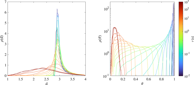
Figure 2. Probability distribution functions ρ(·) of the local dimension d (left panel) and the inverse persistence θ (right panel) as a function of the scale τ (colored lines). For better clarity, we restrict our range of displayed local dimension values to d ∈ [1, 4].
Download figure:
Standard image High-resolution imageWe observe a decrease of both d and θ as τ increases, suggesting that the whole phase-space properties resemble those of a low-dimensional dynamical system. This is again reminiscent of the fluid-dynamical behavior as observed in the turbulent von Karman swirling flow, which despite very high Reynolds number, has been characterized by a low-dimensional stochastic attractor (Faranda et al. 2017). Conversely, larger d and θ characterize the short-term variability of the solar wind magnetic field, providing evidence for an underlying higher-dimensional structure. This seems to suggest a dynamical transition in the underlying structure of the phase space when moving from short- to long-term dynamics, i.e., when passing from kinetic/dissipative to MHD/inertial scales. To better underline these features, we evaluate the average values of d and θ at the different scales τ and compare them with the behavior of S(τ) (see Equation (6)) as reported in Figure 3.

Figure 3. Average values 〈d〉 (left panel, red asterisks) and 〈θ〉 (right panel, red asterisks) at the different scales τ compared with the behavior of S(τ) (blue circles). The gray shaded area marks scales below τnoise ∼ 0.2 s corresponding to the FGM instrumental noise. The vertical dotted black line indicates the scale break at τb ∼ 2.4 s. The dashed–dotted and the dashed lines highlight power-law best fits within the two different scaling regimes: Kolmogorov-like ∼ τ1.69±0.03 for τ > τb and a steeper scaling ∼ τ2.39±0.07 at scales τnoise < τ < τb . Both fits are comparable with the results provided in Roberts et al. (2020a).
Download figure:
Standard image High-resolution imageThe behavior of S(τ) evidences the existence of three different dynamical regimes: the instrumental noise range for τ < τnoise, the kinetic/dissipative range for τnoise < τ < τb , and the MHD/inertial range for τ > τb . These findings are well in agreement with the results of both Bandyopadhyay et al. (2018) and Roberts et al. (2020a). By looking at the behavior of 〈d〉 and 〈θ〉 at the different scales τ we clearly observe a scale-dependent behavior of 〈d〉 that resembles that highlighted by S(τ). The instrumental noise regime is characterized by 〈d〉 = 3 and 〈θ〉 ≈ 1 suggesting, as expected, a purely stochastic origin for the short-term variability of magnetic field fluctuations (i.e., τ < τnoise). From a dynamical system point of view, this means that ergodicity characterizes the phase space, i.e., there exists a reference trajectory of a "typical" point that can be used for deducing the average behavior of the system.
The kinetic/dissipative regime (τnoise
< τ < τb
) is instead characterized by an increasing 〈d〉 as τ increases, reaching a maximum value of  for τ ∼ τb
(i.e., larger than the topological dimension of the system), together with a nonlinearly decreasing 〈θ〉 with rising τ, reaching an inflection point for τ ∼ τb
. These features have not been reported before in the literature and can be interpreted as an increase in the average number of degrees of freedom at kinetic/dissipative scales due to the nonlinear energy cascade effects being characterized by a net energy transfer toward these scales (Kolmogorov 1941). Moreover, the behavior of 〈d〉 and 〈θ〉 at τ ∼ τb
is clearly the reflection of a transition in the dynamical behavior occurring at the boundary between the kinetic/dissipative and the MHD/inertial regimes. Indeed, going toward larger scales (i.e., approaching the MHD/inertial range), we observe a decreasing 〈d〉 and 〈θ〉 with increasing τ, reflecting a reduced-order nature of large-scale magnetic field fluctuations with an active number of degrees of freedom that is lower than the topological dimension of the system (〈d〉 < 3). This points toward the possibility to describe the dynamics across the inertial range as a low-dimensional dynamical system (Alberti et al. 2019). Furthermore, the reduced values of 〈θ〉 suggest a long residence time of the system in the dynamical states corresponding to the inertial range, indicating that they can be interpreted as a collection of marginally stable fixed points of the dynamics with kinetic/dissipative scale induced transitions. Taking together the above results, we can firmly state that (i) the inertial range dynamics can be easily described as a reduced-order dynamical system, and (ii) the increasing dimensionality of the kinetic/dissipative regime is a reflection of small-scale turbulence-induced magnetic field fluctuations due to a dynamical component that is external to the kinetic/dissipative physics, i.e., dynamical information is introduced from processes occurring through the inertial regime and reflecting a direct energy cascade mechanism.
for τ ∼ τb
(i.e., larger than the topological dimension of the system), together with a nonlinearly decreasing 〈θ〉 with rising τ, reaching an inflection point for τ ∼ τb
. These features have not been reported before in the literature and can be interpreted as an increase in the average number of degrees of freedom at kinetic/dissipative scales due to the nonlinear energy cascade effects being characterized by a net energy transfer toward these scales (Kolmogorov 1941). Moreover, the behavior of 〈d〉 and 〈θ〉 at τ ∼ τb
is clearly the reflection of a transition in the dynamical behavior occurring at the boundary between the kinetic/dissipative and the MHD/inertial regimes. Indeed, going toward larger scales (i.e., approaching the MHD/inertial range), we observe a decreasing 〈d〉 and 〈θ〉 with increasing τ, reflecting a reduced-order nature of large-scale magnetic field fluctuations with an active number of degrees of freedom that is lower than the topological dimension of the system (〈d〉 < 3). This points toward the possibility to describe the dynamics across the inertial range as a low-dimensional dynamical system (Alberti et al. 2019). Furthermore, the reduced values of 〈θ〉 suggest a long residence time of the system in the dynamical states corresponding to the inertial range, indicating that they can be interpreted as a collection of marginally stable fixed points of the dynamics with kinetic/dissipative scale induced transitions. Taking together the above results, we can firmly state that (i) the inertial range dynamics can be easily described as a reduced-order dynamical system, and (ii) the increasing dimensionality of the kinetic/dissipative regime is a reflection of small-scale turbulence-induced magnetic field fluctuations due to a dynamical component that is external to the kinetic/dissipative physics, i.e., dynamical information is introduced from processes occurring through the inertial regime and reflecting a direct energy cascade mechanism.
To further support the claim that a larger number of degrees of freedom in magnetic field fluctuations is only due to processes occurring at kinetic/dissipative scales while global properties are mainly related to MHD/inertial processes, we compare the behavior of the d–θ plane at two different scales, τD ∼ 0.6 s and τI ∼ 102 s, belonging to the kinetic/dissipative and the MHD/inertial regimes, respectively, in dependence on the ratio between magnetic field fluctuations at that scale and their standard deviation as reported in Figure 4.
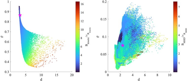
Figure 4. d–θ plane at two different scales τD ∼ 0.6 s (left) and τI ∼ 102 s (right) in dependence on the ratio between magnetic field fluctuations at that scale and their standard deviation (colors). The magenta stars correspond to the mean values of d and θ at the two different scales.
Download figure:
Standard image High-resolution imageWe observe that larger values of d are associated with larger fluctuations at kinetic/dissipative scales, thus suggesting a key role of the organization of kinetic/dissipative scales in regulating the active number of degrees of freedom of the system. We also show that a very wide range of θ values is observed at kinetic/dissipative scales, thus reflecting an unstable (from a dynamical system point of view) nature of fluctuations within this regime. Conversely, when inertial scales are reached we evidence a reduced range of θ, confined below 0.2, together with a clearly narrower range of d with respect to the kinetic/dissipative regime. This suggests that the MHD dynamics is dominated by marginally stable fixed points conferring a low-dimensional nature to the system.
To quantitatively demonstrate these observations, we evaluated the mutual information between d (θ) and  (Equation (7)). Given two signals s1(t) and s2(t) the mutual information is defined as

where p(s1, s2) is the joint probability of observing the pair of values (s1, s2), while p(s1) and p(s2) are the marginal distributions (Shannon 1948). For statistically independent time series M i = 0, while for statistically significantly correlated time series M i ≥ M i th being M i th a threshold associated with a particular statistical significance level (e.g., 95%). We use Kernel Density Estimator (KDE) methods for evaluating probability distributions, i.e., a non-parametric estimator providing smoothed distributions (Silverman 1986), while M i th is evaluated by randomly sampling data points with replacement (i.e., via a bootstrapping procedure; Efron 1979). As shown in Figure 5 a statistically significant dependency is clearly found between d and magnetic field fluctuations below the break scale τb as well as between θ and the MHD/inertial range dynamics (τ > τb ). This quantitatively shows that the overall dynamics of solar wind magnetic field variability reflects those observed at MHD/inertial scales, being characterized by a low-dimensional dynamics around marginally stable fixed points, while a larger number of degrees of freedom in conjunction with an unstable nature of the phase-space topology reflecting an externally forced dynamics is associated with the kinetic/dissipative range dynamics. The electron scales contributions (if any) to the dynamics remain difficult to evaluate because of the prominent role of the noise overriding the dynamics at these smaller scales.

Figure 5. Mutual information between d and  (red) and between θ and
  (green). The gray shaded area marks scales below τnoise ∼ 0.2 s corresponding to the FGM instrumental noise. The vertical dotted black line indicates the scale break at τb
∼ 2.4 s. The horizontal violet shaded area denotes the 95% significance level.
(green). The gray shaded area marks scales below τnoise ∼ 0.2 s corresponding to the FGM instrumental noise. The vertical dotted black line indicates the scale break at τb
∼ 2.4 s. The horizontal violet shaded area denotes the 95% significance level.
Download figure:
Standard image High-resolution image
4. Conclusions
Our results provide evidence that the number of degrees of freedom in the solar wind magnetic field variations at kinetic/dissipative scales (τ < τb ) is larger than the topological dimension of the system (D = 3), while a low-dimensional phase space is found at MHD/inertial scales (τ > τb ). On the one hand, this suggests the existence of an externally induced dynamics at kinetic/dissipative scales that can be related to the inertial range direct cascade mechanism; on the other hand, this also implies that there exists a degree of correlation between magnetic field components that tends to reduce the effective number of degrees of freedom at MHD scales. The latter result points toward a quasi-2D nature of magnetic field fluctuations at MHD scales with an inverse enstrophy cascade typically arising in near two-dimensional incompressible decaying turbulence. Taken together, we firmly demonstrated that sudden variations observed in magnetic field measurements are associated with unstable fixed points characterizing the dynamics at kinetic/dissipative scales. These large-scale intermittency-like variations cannot be definitely associated with coherent intermittent events belonging to the MHD domain, but seem to be related to an underlying stochastic strange attractor (Carbone et al. 2021), in close analogy with the results obtained by Raphaldini et al. (2020, 2021) for MHD and Faranda et al. (2017) for fluid turbulence. Indeed, we also demonstrated the existence of a different fixed point nature across the different scales, moving from an unstable point approached at kinetic/dissipative scales to marginally stable fixed points at inertial scales. Thus, the overall dynamics of solar wind magnetic field fluctuations consists of multistable and multiscale fixed points, opening a novel way to describe the solar wind via stochastic low-dimensional models featuring a large number of degrees of freedom (Faranda et al. 2017; Carbone et al. 2021). Finally, our results are in agreement with previous findings on the possibility of using low-order models (e.g., cascade models) to describe energy transfer across the MHD domain; on the other side, our findings shed new light on the investigation of the underlying fractal topology at small scales, pointing toward the existence of a finer topological structure due to the breakdown of the fluid-like/MHD approximation, associated with singularities of the dissipation field. Further investigations will be devoted to the latter topic in a dedicated future work.
We acknowledge the MMS team and instrument leads for data access and support. The data presented in this paper are the L2 data of MMS and can be accessed from the MMS Science Data Center (https://lasp.colorado.edu/mms/sdc/public/). T.A., R.V.D., and G.C. acknowledge fruitful discussions within the scope of the International Team "Complex Systems Perspectives Pertaining to the Research of the Near-Earth Electromagnetic Environment" at the International Space Science Institute in Bern, Switzerland. V.C. and G.C. acknowledge financial support from the Italian MIUR-PRIN grant 2017APKP7T on "Circumterrestrial Environment: Impact of Sun-Earth Interaction". R.V.D. has received support by the German Federal Ministry for Education and Research of Germany (BMBF) via the JPI Climate/JPI Oceans project ROADMAP (grant No. 01LP2002B). We are particularly grateful to the anonymous reviewer for constructive and helpful comments and suggestions.