


Abstract
The NANOGrav Collaboration reported strong Bayesian evidence for a common-spectrum stochastic process in its 12.5 yr pulsar timing array data set, with median characteristic strain amplitude at periods of a year of  . However, evidence for the quadrupolar Hellings & Downs interpulsar correlations, which are characteristic of gravitational-wave signals, was not yet significant. We emulate and extend the NANOGrav data set, injecting a wide range of stochastic gravitational-wave background (GWB) signals that encompass a variety of amplitudes and spectral shapes, and quantify three key milestones. (I) Given the amplitude measured in the 12.5 yr analysis and assuming this signal is a GWB, we expect to accumulate robust evidence of an interpulsar-correlated GWB signal with 15–17 yr of data, i.e., an additional 2–5 yr from the 12.5 yr data set. (II) At the initial detection, we expect a fractional uncertainty of 40% on the power-law strain spectrum slope, which is sufficient to distinguish a GWB of supermassive black hole binary origin from some models predicting more exotic origins. (III) Similarly, the measured GWB amplitude will have an uncertainty of 44% upon initial detection, allowing us to arbitrate between some population models of supermassive black hole binaries. In addition, power-law models are distinguishable from those having low-frequency spectral turnovers once 20 yr of data are reached. Even though our study is based on the NANOGrav data, we also derive relations that allow for a generalization to other pulsar timing array data sets. Most notably, by combining the data of individual arrays into the International Pulsar Timing Array, all of these milestones can be reached significantly earlier.
Export citation and abstract BibTeX RIS
1. Introduction
Supermassive black hole binaries (SMBHBs) are expected to form following the mergers of massive galaxies during the buildup of hierarchical structure in ΛCDM (Burke-Spolaor et al. 2019, and references therein). No observationally confirmed SMBHBs at subparsec separations are known, but a growing number of strong candidates have been identified (Graham et al. 2015; Charisi et al. 2016; Liu et al. 2019; Chen et al. 2020). If SMBHBs are indeed able to form, and also to reach ∼milliparsec separations, then they will become the sources of the strongest gravitational waves (GWs) in the universe. The stochastic superposition of GWs produced by SMBHBs across cosmic time is expected to produce an aggregate background signal with an approximate characteristic strain spectrum of the form  with α = −2/3 for a continuous population of circular and purely GW-driven binary systems (Rajagopal & Romani 1995; Jaffe & Backer 2003; Sesana et al. 2008). At low frequencies (f ≲ 10−8 Hz), interactions between SMBHBs and their ambient galactic environments can turn over or flatten the spectrum (α > −2/3; Sampson et al. 2015; Kelley et al. 2017b; Taylor et al. 2017). At high frequencies (f ≳ 10−8 Hz), rapid binary hardening can lead to a low occupation of spectral bins that steepens the spectrum (α < −2/3) and may introduce spikes from individual sources (Sesana et al. 2008). Despite these effects, the stochastic GW background (GWB) from SMBHBs is expected to be the dominant source of GWs in the nanohertz frequency regime.
Pulsar Timing Arrays (PTAs; Sazhin 1978; Detweiler 1979; Foster & Backer 1990) measure the times of arrival (TOAs) of radio pulses from millisecond pulsars as a means of measuring the local spacetime curvature, and thus signs of passing GWs, analogous to how the LIGO-Virgo Collaboration (Harry & LIGO Scientific Collaboration 2010; Accadia et al. 2012) uses pairs of perpendicular laser arms. As PTAs accrue larger data sets over time, the increasing number of recorded pulses leads to improved sensitivity, especially as new pulsars are added to the arrays (Siemens et al. 2013; Taylor et al. 2016). The NANOGrav 12.5 yr data set (Alam et al. 2021) shows conclusive evidence (with Bayesian odds of ∼104:1) that a common-spectrum low-frequency stochastic process is present across a large fraction of the 45 ms pulsars included in the analysis (Arzoumanian et al. 2020). Its properties are consistent with expectations of the strain spectrum from a stochastic GWB, but it does not yet show statistically significant quadrupolar interpulsar correlations, which are widely considered the definitive evidence for the GWB (Hellings & Downs 1983; Tiburzi et al. 2016). The latter are the so-called "Hellings & Downs" (HD) correlations of GWB-induced timing delays between pairs of pulsars, which are a function only of the angular separation between the pulsars on the sky. Future data sets, such as the in-preparation NANOGrav 15 yr data set, in addition to data from the European PTA (EPTA; Desvignes et al. 2016), Australian Parkes PTA (PPTA; Kerr et al. 2020), and the International Pulsar Timing Array (IPTA; Verbiest et al. 2016; Perera et al. 2019), will reveal the nature of the signal. These data will either show spatial correlations consistent with a GWB, or other correlation signatures that suggest unmodeled noise processes affecting the PTA data.
In this paper, we forecast the evolution of GWB inference into the future, under the assumption that the signal is produced by cosmological SMBHBs. There may be alternate sources of the GWB, and there have been many recent suggestions of such interpretations for the NANOGrav 12.5 yr results (see, e.g., Blasi et al. 2021; De Luca et al. 2021; Ellis & Lewicki 2021; Vaskonen & Veermäe 2021). The scaling results that we derive here are generalizable to such other sources of the GWB. Similar analyses performed in the past were focused only on the time to detection of the GWB (e.g., Taylor et al. 2016; Rosado et al. 2015; Vigeland & Siemens 2016; Kelley et al. 2017b), and while this remains important (especially given the results in Arzoumanian et al. 2020), we consider here for the first time the evolution of the GWB parameter measurement uncertainties. The evolution of these properties is of crucial importance in determining the source and underlying physics that produces the GWB. For example, while a GWB from SMBHBs produces a spectral index of α = −2/3, a GWB produced by primordial GWs can have a spectral index, α = −2 or −1 (Grishchuk 2005; Lasky et al. 2016), while a GWB produced by some models of cosmic strings have α = −7/6 (Ölmez et al. 2010). A distinction between these source models can only be made once the spectral index measurement uncertainty is small enough to exclude one (or more) of the predicted spectral indices. Similarly, different models of a given source can produce different amplitudes of the GWB, and thus knowing when we can distinguish between them is dependent on the evolution of the measurement uncertainties on the GWB amplitude.
However, for a background produced by inspiraling SMBHBs, the canonical α = −2/3 spectral index GW strain power law emerges when assuming a continuous distribution of circular binary sources evolving purely due to GW emission (Phinney 2001). Following galaxy mergers, two SMBHs can only become bound and reach the small separations (≲10−2 pc) required to produce detectable GWs through environmental interactions, such as dynamical friction and stellar "slingshot" scattering (Begelman et al. 1980). These interactions make binaries harden faster than they would due purely to GW emission, and thus the resulting GW strain can be lower than in the −2/3 power law, particularly at low frequencies (f ≪ 1 yr−1). At higher frequencies, finite number effects (Sesana et al. 2008) can also cause significant deviations from a pure power law. We explore the effects of these variations in the SMBHB GWB spectrum by injecting and recovering "realistic" spectra that have been produced through full mock populations of SMBH binaries.
The paper is structured as follows. In Section 2, we describe the methods used to simulate and analyze the PTA data sets. In Section 3, we show that the Bayesian model odds ratio can be related to the frequentist signal-to-noise ratio (S/N) through a simple analytic expression for PTAs, while in Section 4, we derive a new statistic, the total S/N, that encapsulates the information in both the auto- and cross-correlation components of the PTA data. In Section 5, we describe the evolution of the GWB detection significance, parameter uncertainties, and spectral characterization of the GWB, and define three key milestones that PTAs should achieve along the way. Finally, in Section 6, we show how the timeline for achieving these milestones described can be accelerated by combining the data from individual PTAs into the IPTA.
2. Methods
2.1. Simulation Framework
We have developed a framework for realistic pulsar timing data simulation that employs the NANOGrav 12.5 yr data set (Alam et al. 2021) as its foundation, deriving observational time stamps and TOA uncertainties from all 45 pulsars therein, as well as useful metadata such as observing radio frequency and telescope. We account for pulse-phase jitter noise, as well as the usual TOA uncertainties from radiometer noise, using the maximum likelihood pulsar noise parameters measured by NANOGrav in the 12.5 yr data preparation and analysis. We epoch-average the TOA uncertainties and time stamps, which reduces the effective number of TOAs by almost an order of magnitude. We also inject intrinsic red noise in each pulsar according to its measured values in the NANOGrav 12.5 yr data set, with the caveat that we filter out a GWB-like α = −2/3 red process from each pulsar by modeling it alongside the intrinsic pulsar noise. This is important in isolating the true intrinsic red noise in each pulsar, which may otherwise be conflated with a common process in single-pulsar noise estimation. These simulations are the first to inject red noise in each pulsar that reflects the measured NANOGrav common red noise being appropriately filtered out.
In order to forecast data accumulation beyond the existing 12.5 yr baseline, we derive distributions of the observational cadences and TOA uncertainties from the final year's worth of data in each pulsar. We then adopt a status quo approach of drawing new observation times and uncertainties from these distributions until we reach a 20 yr array baseline. We retain the 45 pulsars from the 12.5 yr analysis and do not add any new pulsars as a function of time. This latter choice implies that the temporal growth rate of the detection statistics that we derive in this work will be relatively conservative because the addition of pulsars to the PTA is known to increase the detection significance of the GWB (Siemens et al. 2013).
Finally, we inject ten different realizations of noise and isotropic GWB signals (with spectral index α = −2/3) for each of eight different amplitudes in the range 10−16 ≤ AGWB ≤ 5 × 10⁻¹⁵ into our synthesized 20 yr baseline array. We then study how the signal evolves in our data by analyzing increasingly longer slices of each simulation, from 10 yr up to the final 20 yr. Put together, our PTA simulation technique is the most sophisticated that has ever been presented in the literature.
2.2. Bayesian Data Analysis Methods
The methods used for modeling the injected GWB are the same as those used in the NANOGrav 11 yr (Arzoumanian et al. 2018) and 12.5 yr (Arzoumanian et al. 2020) analyses. Thus, we only briefly summarize the probabilistic framework for estimating the GWB parameters. In the standard detection pipeline, the GWB is modeled as a power law across frequency for the characteristic strain,
where AGWB is the amplitude of the GWB, f is the frequency, and α = −2/3 is the spectral index expected for a population of inspiraling SMBHBs whose inspiral is dominated by GWs. This GWB spectrum can be expressed in terms of the timing-residual cross-spectral density between pulsars a and b as,
where γ ≡ 3 − 2α, and Γab is the overlap reduction function that encodes the interpulsar spatial correlations, such as the HD spatial correlations (Hellings & Downs 1983) expected for an isotropic GWB.
In addition to the GWB, we also need to model the intrinsic noise for each pulsar in the PTA. For each pulsar, we model uncorrelated instrumental Gaussian noise in the multiplicative EFAC and quadrature-additive EQUAD parameters. Noise that is correlated across observing frequencies but uncorrelated across TOAs is modeled using the ECORR parameter. These parameters are collectively referred to as "white noise." We include an additional power-law process per pulsar to model any intrinsic low-frequency noise (i.e., "spin red noise") in the given pulsar. The aforementioned white-noise parameters that correct the reported TOA uncertainties were folded into the simulated uncertainties in the preparation of our data sets, so we do not separately model these white-noise parameters in our analysis. The red noise for the pulsars is allowed to vary when we search for the GWB.
The GWB parameter constraints are derived by modeling the GWB as a time-correlated process that is statistically common (i.e., with a common spectrum) but uncorrelated among all pulsars in the PTA. This ignores the influence of interpulsar correlations on GWB parameter constraints, which should be minimal as these are dominated by autocorrelation information in the pulsars. Constraints on the GWB spectral index, α, are reported as marginalized over all parameters, including AGWB, while constraints on AGWB, are reported as marginalized over all noise parameters but conditioned on the fiducial spectral index α = −2/3. The inclusion of HD correlations in the search process is computationally expensive, so we only use it to discriminate whether the observed common red process is from a GWB or other spatially correlated signals like terrestrial clock errors (monopolar spatial correlations) or solar system ephemeris errors (dipolar spatial correlations). These spatial correlations are encoded in the overlap reduction function in Equation (2).
To calculate the Bayesian detection significance, we use a product-space sampling method that computes the probabilistic preference for one signal model over another (Arzoumanian et al. 2018; Taylor et al. 2020, and references therein). We construct a super-model consisting of the union of multiple GWB signal models, where an indexing variable determines which model is "active" and used to calculate the corresponding likelihood. The ratio of the posterior probabilities of the model indices can then be used to estimate the Bayesian odds for the preference of one model over the other. Thus, to calculate the Bayesian odds for an HD-correlated process in the data set,  , we create a super-model with the same GWB parameters in both models, while the index parameter toggles the presence of HD correlations.
In addition to power-law strain spectrum models, we also measure the GWB strain spectrum agnostically with an independent amplitude at each frequency. Our priors correspond to independent log-uniform constraints on the characteristic strain amplitude for each Fourier-basis frequency, given by k/T, where k = 1, 2,..., 30, and T is the time span between the first and last TOA in the given data set. Unless explicitly specified, all of the results presented in this paper have been derived using 30 frequencies to model the GWB (and intrinsic red noise) and employing the recent JPL solar system ephemeris, DE438 (Folkner & Park 2018). However, we also explore the effect of using a different number of frequencies and BayesEphem (Vallisneri et al. 2020) in modeling the GWB.
2.3. Frequentist Data Analysis Methods
In addition to the Bayesian pipeline, we also use a frequentist approach to model the GWB (Arzoumanian et al. 2016, 2018). This uses an optimal statistic,  , to measure the amplitude of the GWB, corresponding to the sum of the correlations between pulsar pairs weighted by the intrinsic pulsar noise, and conditioned on the assumed spectral index of the GWB. The optimal statistic can also be used to calculate the S/N, ρtemplate, for a given interpulsar correlation template, e.g., monopolar or dipolar for clock and ephemeris errors, respectively, and HD (or quadrupolar) for an astrophysical GWB. To calculate the template S/N, the optimal statistic first calculates the amount of cross-correlated power between different pulsar pairs in the PTA. This pairwise cross-correlated power, suitably binned in angular separation space, can be used as a visual test for the presence of quadrupolar correlations in the data, or as intermediate products for further study of the spatial correlations.
In this work, we use the noise-marginalized optimal statistic (Vigeland et al. 2018), which is more robust when pulsars have intrinsic red noise. We use posterior samples from Bayesian MCMC analyses to marginalize over the pulsar intrinsic red noise and calculate corresponding distributions for  and ρtemplate.
These Bayesian and frequentist methods reflect production-level analyses that are employed in PTA detection and parameter estimation analyses. Thus, our results are a crucial validation of the efficacy of the pipelines that will be performing the important business of SGWB detection in the next several years.
3. Bridging Bayesian Odds and Frequentist S/Ns
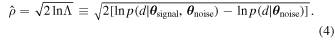
Under certain circumstances, it is possible to relate Bayesian model selection to frequentist hypothesis testing. When data is informative such that the likelihood is strongly peaked, the Bayesian evidence can be computed under the Laplace approximation, such that  , where
  maximizes the likelihood with parameters θ given data d under model
  (Romano & Cornish 2017).
  measures the compactness of the parameter space volume occupied by the likelihood with respect to the total prior volume, incorporating the Bayesian notion of model parsimony. Taking the ratio of the Bayesian evidence between two models, labeled 1 and 2, and assuming equal prior odds, allows the Bayesian odds ratio,
  , to be written as
 ![$\mathrm{ln}{{ \mathcal O }}_{12}\approx \mathrm{ln}{{\rm{\Lambda }}}_{\mathrm{ML}}(d)+\mathrm{ln}\left[({\rm{\Delta }}{V}_{1}/{V}_{1})/({\rm{\Delta }}{V}_{2}/{V}_{2})\right]$](https://content.cld.iop.org/journals/2041-8205/911/2/L34/revision3/apjlabf2c9ieqn11.gif) , where ΛML(d) is the maximum likelihood ratio. The relevant maximum likelihood statistic for PTA GWB detection is the aforementioned optimal statistic: a noise-weighted two-point correlation statistic between all unique pulsar pairs, which compares a model with HD interpulsar correlations versus one with no correlations between pulsars (Anholm et al. 2009; Demorest et al. 2013; Chamberlin et al. 2015). The signal-to-noise ratio (S/N, ρ) of such GWB-induced correlations can be written as
, where ΛML(d) is the maximum likelihood ratio. The relevant maximum likelihood statistic for PTA GWB detection is the aforementioned optimal statistic: a noise-weighted two-point correlation statistic between all unique pulsar pairs, which compares a model with HD interpulsar correlations versus one with no correlations between pulsars (Anholm et al. 2009; Demorest et al. 2013; Chamberlin et al. 2015). The signal-to-noise ratio (S/N, ρ) of such GWB-induced correlations can be written as  . While the likelihood may be marginally more compact under the model with HD correlations, there is no difference in parameter dimensionality; hence, we ignore the likelihood compactness terms. The relationship between the Bayesian odds ratio in favor of HD correlations and the frequentist S/N of such correlations can then be written as

In a bid to assess the validity of this relationship for PTA GWB searches, we used our simulated data sets to calculate both of these statistics across all realizations, injected amplitudes, and time slices. These values, and the theoretical relationship in Equation (3), are shown in Figure 1. We also allowed the prefactor of 1/2 to vary in an empirical fit, finding a value of 0.52 ± 0.01, which agrees well with Equation (3). This is the first time that this relationship has been validated for PTA GWB detection.
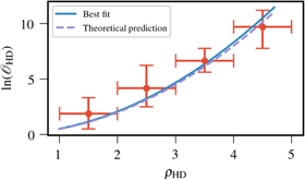
Figure 1. The Bayesian odds ratio preferring a GWB over a spatially uncorrelated process ( ) is plotted against the cross-correlation signal-to-noise ratio (S/N, ρ). These quantities were calculated using the injected simulated data sets across all realizations and injected amplitudes. The theoretical prediction (dashed blue line) for the relation between these two measures of confidence agrees with the empirical best-fit model (solid blue line).
Download figure:
Standard image High-resolution image4. A Statistic to Quantify PTA Milestones
There are many factors that influence the detectability of a GWB signal in a given PTA configuration. Some of these are related to the signal itself, i.e., the amplitude of the characteristic strain spectrum at f = 1/yr, AGWB, as well as the frequency-dependent shape of the spectrum. The quality of our detector is parameterized through the overall observational timing baseline of the array, the number of pulsars, and the timing quality of each pulsar (given by its radio-frequency-dependent noise characteristics). We need a statistic that accounts for all of these factors, acting as a fiducial scaling parameter in terms of which we can track the evolution of parameter uncertainties and signal detectability. The optimal statistic is not appropriate here, because it only considers cross-correlations and thus underestimates the information content in the full signal (especially the autocorrelations) that dominate parameter estimation.
The full signal likelihood (modeling auto- and cross-correlations) is a sufficient statistic for this purpose. Hence, we form a total-signal S/N,  , through the log-likelihood ratio of the GWB+noise versus noise-only models, where noise is treated as uncorrelated between pulsars. Therefore,
This differs from the HD cross-correlation S/N, ρHD (or an equivalent cross-correlation statistic) in considering all distinct pairings of the pulsars, including autocorrelations.
We would like to note that this new statistic is not meant to be a replacement for the cross-correlation S/N. Because an astrophysical GWB is characterized by the unique HD cross-correlation signature, the corresponding cross-correlation S/N, ρHD, will be the primary arbiter for confirming a signal as an astrophysical GWB.
As PTAs move closer to detection, the power in the GWB at low frequencies is expected to dominate the intrinsic white and red noise in some of the pulsars in the PTA. In this "intermediate-signal regime," the total S/N,  , is expected to be much larger than the corresponding HD S/N (ρHD, Romano et al. 2020). We can directly connect them by calculating the two statistics on the same simulated injected data sets. The binned values for the two statistics calculated this way are shown in Figure 2 and related by the empirical scaling relation
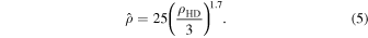
Using this scaling relation, ρHD values of [1, 3, 7] map to  values of approximately [5, 25, 105] respectively. Because the power in autocorrelations is significantly larger than that in cross-correlations, the corresponding S/N values for the total SN,
  , are higher than those for HD cross-correlation, ρHD (Romano et al. 2020).
Figure 2. The evolution of the total S/N,  , as a function of the HD cross-correlation S/N, ρHD. As we can see, HD template S/N values of 1, 3, and 7 correspond to
  values of 5, 25, and 105 respectively.
Download figure:
Standard image High-resolution imageFrom existing scaling laws for ρHD (Siemens et al. 2013), we can generalize  to any PTA configuration. For a PTA in the weak- and intermediate-signal regime (Siemens et al. 2013), the total S/N can be written as
respectively, where M is the number of pulsars in the array, c = 1/Δt is the inverse of the observational cadence, AGWB is the amplitude of the GWB, σ is the white-noise timing rms, T is the timing baseline of the PTA, and γ is as previously defined (γ ≡ 3 − 2α = 13/3 for a population of SMBHBs).
5. PTA Milestones
5.1. Milestone I: Detection
The upper panel of Figure 3 shows the evolution of the median  as a function of data baseline and injected GWB amplitude, the middle panels show the cross-correlated power in different angular separation bins for a GWB with an amplitude of AGWB = 2 × 10⁻¹⁵ 2 for three different data baselines (12, 15, and 20 yr), and the lower panel shows the evolution of the S/N for HD, monopole, and dipole cross-correlations as a function of data baseline for a GWB with amplitude between AGWB = [1–2] × 10−15. With an increase in the length of the PTA data set,
  for the GWB increases, as well as the S/N for HD correlations, ρHD. The bottom panel of Figure 3 shows that, starting at the 15 yr slice, the median HD correlations are preferred over other types of spatial correlation for a GWB with strength AGWB = [1–2] × 10−15. Only with HD correlations clearly favored over monopolar or dipolar signals (which happens near the 18 yr baseline in our simulations) can a signal be confidently attributed to GWBs instead of uncharacterized noise sources.

Figure 3. Top: the evolution of the median total S/N,  , over 10 realizations as a function of time. The dashed–dotted, dashed, and solid contours represent total S/N values of 5, 25, and 105 corresponding to HD S/Ns, ρHD, of 1, 3, and 7 respectively. The black data point represents the amplitude of the GWB from the NANOGrav 12.5 yr analysis. Middle: the median binned cross-correlated power over 10 realizations for increasing S/N from left to right. The uncertainties in this panel represent the spread of the cross-correlated power over the 10 realizations. The theoretical HD curve for a power-law GWB with an amplitude of AGWB = 2 × 10⁻¹⁵ is shown by the red dashed line. Bottom: the cross-correlation S/N ratio, ρtemplate, for different types of spatial correlations with an injected power-law GWB amplitude of AGWB = [1–2] × 10−15. The shaded regions represent the median 95% credible intervals across ten realizations of the PTA data set. The black data point represents the significance of the GWB from the NANOGrav 12.5 yr analysis.
Download figure:
Standard image High-resolution imageTo test the influence of the number of frequencies used to model the GWB, we repeat the analysis in the lower panel of Figure 3 for a GWB modeled with only the five lowest frequencies. The choice of these five lowest frequencies is designed to avoid GWB significance and parameter estimation being contaminated by poorly modeled excess noise in the data set that dominates at higher frequencies (Arzoumanian et al. 2020). We find that the initial detection of a GWB is not inhibited or delayed by using only the five lowest frequency bins, which only reduces the S/N for HD correlations by a few percent. We also explored the influence that accounting for systematics in solar system ephemeris modeling has on our GWB detection significance. We do so by including BayesEphem (Vallisneri et al. 2020) in our model, which marginalizes over uncertainties in Jupiter orbital elements, gas giant masses, and the celestial reference frame. We find that BayesEphem reduces detection significance by only ∼4 units of total S/N,  , consistent with earlier results reported in Vallisneri et al. (2020). Thus, the presence of solar system ephemeris uncertainties is unlikely to inhibit the detection of a GWB by PTAs.
As shown in Figure 3 as a black data point, detection statistics for the NANOGrav 12.5 yr data set are consistent with our simulations, and we expect the significance of a GWB to increase in the real data set at least at the rate shown here, if not faster due to the addition of more pulsars to the array (Siemens et al. 2013) and new advanced noise mitigate schemes that should allow the GWB spectrum to be modeled to higher frequencies.
5.2. Milestone II: Source of The GWB
Figure 4 shows the evolution of the fractional parameter measurement uncertainty, ΔX/X, as a function of total S/N, where X is the median measured value of the GWB amplitude (AGWB) and spectral index (α), and ΔX is the corresponding 95% credible interval parameter uncertainty. These uncertainties are well fit by the relations,
The choice of using the five lowest frequencies to model the GWB does not affect the fractional parameter uncertainties until the signal has total S/N  , whereupon using 30 frequencies improves their recovery. At such high detection significance, the GWB begins to dominate more than just the five lowest frequency bins, accruing greater significance and more informative constraints from higher frequencies. We also find that the inclusion of BayesEphem has a minimal effect on the fractional uncertainty of the measured GWB parameters.
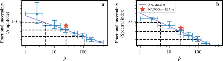
Figure 4. The evolution of the median fractional uncertainty on the measured amplitude, A, and spectral index, α, as a function of total S/N,  , is shown in panels (a) and (b), respectively. The evolution of the fractional uncertainty for the amplitude and spectral index with the S/N is best fit by a power law as shown (parameterized in Equation (7)). For the amplitude and spectral index, the fractional uncertainties corresponding to
  values of 5, 25, and 105 are 84%; 44% and 25%; and 90%, 40%, and 20%, respectively, and are shown by the dashed black lines. The star shows the fractional uncertainty from the NANOGrav 12.5 yr analysis.
Download figure:
Standard image High-resolution imageThe measured spectral index of the GWB will be the primary arbiter of the source of the GWB. A spectral index of α = −2/3, corresponding to our injected signal, is expected for a purely GW-driven population of inspiraling SMBHB systems, while other more exotic sources of the GWB are predicted to have different spectral indices. At initial detection ( or ρHD = 3), the spectral index measurement should have a fractional uncertainty of 40% (Equation 7(b)). In our suite of simulations, this precision is already sufficient to disfavor (at 95% credibility) models of primordial GWs with matter (α = −2; Grishchuk 2005) and radiation-dominated (α = −1; Lasky et al. 2016) equations of state.
43
This precision is also sufficient to disfavor some models of the GWB produced by cosmic strings, such as those from kinks and cusps in the string loops, which are predicted to have a spectral index, α = −7/6 (Ölmez et al. 2010). As the significance of the GWB signal grows, the fractional uncertainty on the measured spectral index will continue to decrease and allow us to test other sources of the GWB. As we show later, an increase in the timing baseline of the data set allows more comprehensive spectral modeling of the GWB, thereby reducing the need to rely on power-law fits.
or ρHD = 3), the spectral index measurement should have a fractional uncertainty of 40% (Equation 7(b)). In our suite of simulations, this precision is already sufficient to disfavor (at 95% credibility) models of primordial GWs with matter (α = −2; Grishchuk 2005) and radiation-dominated (α = −1; Lasky et al. 2016) equations of state.
43
This precision is also sufficient to disfavor some models of the GWB produced by cosmic strings, such as those from kinks and cusps in the string loops, which are predicted to have a spectral index, α = −7/6 (Ölmez et al. 2010). As the significance of the GWB signal grows, the fractional uncertainty on the measured spectral index will continue to decrease and allow us to test other sources of the GWB. As we show later, an increase in the timing baseline of the data set allows more comprehensive spectral modeling of the GWB, thereby reducing the need to rely on power-law fits.
5.3. Milestone III: Properties of The GWB
Once there is sufficient evidence that the GWB is most likely due to a population of merging SMBHBs, we can use our spectral characterization to probe the astrophysics of the underlying SMBHB population. For example, the amplitude of a GWB produced by SMBHBs is set primarily by the mass distribution of SMBHs, often parameterized relative to their host galaxies (e.g., in the M–σ relation; Ferrarese & Merritt 2000; Gebhardt et al. 2000), and the efficiency by which they reach subparsec separations. The recovered amplitude can thus be used to distinguish between different population models of SMBHBs.
Here we consider three such models (McWilliams et al. 2014; Sesana et al. 2016; Simon & Burke-Spolaor 2016) with GWB amplitudes representative of typical values predicted in the literature: ![${A}_{\mathrm{GWB}}=\left[{0.4}_{-0.16}^{+0.26},{1.5}_{-0.3}^{+0.3},{4.0}_{-1.8}^{+3.3}\right]\times {10}^{-15}$](https://content.cld.iop.org/journals/2041-8205/911/2/L34/revision3/apjlabf2c9ieqn29.gif) , which were also examined in the NANOGrav 11 yr GWB analysis (Arzoumanian et al. 2018). At initial detection, the amplitude measurement will have a fractional uncertainty of 44%, which will be sufficient to distinguish the first model from the other two. Models two and three are distinguishable with a fractional uncertainty of ∼37% on the amplitude, occurring near the 17 yr slice of our simulated data. Thus, almost immediately after the initial detection of the GWB, we expect to be able to clearly distinguish between typical models in the literature.
, which were also examined in the NANOGrav 11 yr GWB analysis (Arzoumanian et al. 2018). At initial detection, the amplitude measurement will have a fractional uncertainty of 44%, which will be sufficient to distinguish the first model from the other two. Models two and three are distinguishable with a fractional uncertainty of ∼37% on the amplitude, occurring near the 17 yr slice of our simulated data. Thus, almost immediately after the initial detection of the GWB, we expect to be able to clearly distinguish between typical models in the literature.
5.3.1. Constraining Dynamical Influences on the GWB Spectral Shape
A realistic, astrophysical GWB from SMBHBs is, however, expected to deviate noticeably from the pure power-law spectrum we have assumed so far. To quantify the influence of these deviations on our detection prospects, we use astrophysically motivated simulations of SMBHB populations to inject three non-power-law GWB spectra into the synthesized data.
To calculate plausible and self-consistent GWB spectra, we generate full mock populations of SMBH binaries. We employ two entirely independent approaches to simulate SMBHB populations. In the first, we anchor the population on the galaxy–galaxy merger rate derived from the Illustris cosmological simulations (Genel et al. 2014; Vogelsberger et al. 2014a, 2014b). While the Illustris population of SMBH mergers has been used extensively (Kelley et al. 2017a, 2017b, 2018), we have generalized our approach to allow for a more flexible range of binary properties and thus resulting GWB spectra. In particular, we have chosen binary hardening rates and masses so as to produce (i) a GWB spectrum that is very nearly a power law with a relatively steep "negative" spectral index at low frequencies (Figure 5: gray), and (ii) a strain spectrum that is nearly "flat" at low frequencies (Figure 5: yellow).
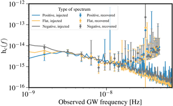
Figure 5. Per-frequency spectral modeling of the GWB spectrum for the 20 yr slice. Each frequency bin shows the median strain and uncertainty across 10 realizations, while the injected GWB spectrum is shown by the solid lines. The few lowest frequency bins closely track the shape of the injected GWB, with the lowest frequency bin being the strongest discriminator between the three types of injected spectra. The high-frequency bins are dominated by the white noise in the PTA and thus are insensitive to the GWB.
Download figure:
Standard image High-resolution imageThe second method uses spectra originally generated for the astrophysical inference performed on the NANOGrav 11 yr data set (Arzoumanian et al. 2018). This method uses a semi-analytic model (Simon & Burke-Spolaor 2016) to simulate a binary population using observational-based measurements of the galaxy stellar mass function, galaxy merger rate, and SMBH mass–host galaxy relation. The eccentricity distribution and binary hardening rate is incorporated over a wide range of parameters (Taylor et al. 2017). Model parameters are chosen to produce (iii) a GW strain spectrum that is attenuated strongly enough to turn over, producing a "positive" spectral index at low frequencies (Figure 5: blue).
Overall, the amplitude of the simulated spectra is calibrated primarily by the distribution of SMBH masses, and the low-frequency spectral index is increased from the fiducial −2/3 by increasing the environmental hardening rate, mostly due to coupling with the nuclear stellar environment (Simon & Burke-Spolaor 2016; Kelley et al. 2017b). For both methodologies, we have calibrated all three realistic spectra to have an amplitude of AGWB = 1 × 10⁻¹⁵ at a frequency of 1 yr−1 and are shown by the solid lines in Figure 5.
The total S/N recovered using our standard detection pipeline (assuming a pure power-law strain spectrum) is shown for these realistically modeled GWB spectra in Figure 6. Even in the "positive" model, where a significant amount of GW strain is attenuated at low frequencies, the measured S/N is unaffected at the 15–17 yr slices (where initial detection is predicted to happen) and is only decreased by ∼50% at the 20 yr slice. This point is crucial because it demonstrates that the assumption of a pure power-law strain spectrum allows for a high S/N detection, despite omitting the detailed spectral structure. Additionally, even significant attenuation of the GWB signal at low frequencies does not represent a significant obstacle to detection. Any eventual reduction in the recovered S/N compared to the predicted S/N can then be used to interpret the presence of a turnover in the GWB spectrum.
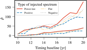
Figure 6. Detection significance for a variety of injected GWB spectra that are all modeled using a pure power-law spectrum in the detection pipeline. The two sets of curves represent the median 95% credible interval upper and lower bounds on the S/N. We can see that power-law modeling of the GWB is robust for making a detection of the GWB.
Download figure:
Standard image High-resolution imageHowever, many of the astrophysical details about SMBHB environments and demographics are missed by power-law analyses. The additional encoded information can be extracted using per-frequency modeling of the GWB (Lentati et al. 2013; Taylor et al. 2013). In this approach, the strain in each frequency bin is modeled independently, allowing us to measure the spectral shape of the underlying GWB. A per-frequency spectral analysis of 20 yr of data is shown in Figure 5 for our three astrophysically motivated injected GWB spectra, with points and uncertainties representing strain measured independently in each frequency bin. We see that the few lowest bins are dominated by the injected GWB and closely track their spectral shapes. In a follow-up analysis, we will explore full astrophysical model inference to determine how accurately astrophysical parameters can be extracted from realistic GWBs. However, the results shown here are very encouraging in that even models with some degeneracy (i.e., in the overall signal amplitude, AGWB) can be disentangled within the next several years.
6. Accelerating PTA Milestones
The S/N for a GWB signal in PTA data can be raised by increasing either the time span of the data set or the number of monitored pulsars (Siemens et al. 2013). However, new pulsars usually cannot be added into a PTA immediately upon discovery and generally require multiple years of timing data to assess their appropriateness for PTA analysis. A solution is to combine the data already collected by PTAs around the world into a single data set and analyze this joint data set for a GWB signal. Beyond NANOGrav, there are currently two other PTAs apart that have decades' worth of timing data on millisecond pulsars: the Parkes Pulsar Timing Array (PPTA; Hobbs 2013) and the European Pulsar Timing Array (EPTA; Kramer & Champion 2013). Together, these PTAs, along with emerging PTAs in India (InPTA; Joshi et al. 2018), China (CPTA, Lee 2016) and South Africa (SAPTA; Bailes et al. 2016), form the International Pulsar Timing Array (IPTA; Hobbs et al. 2010). To date, the IPTA has published two data releases (Verbiest et al. 2016; Perera et al. 2019), which result in an increase in the number of pulsars relative to individual regional PTAs at that time, while also increasing the time span of data for pulsars that are common across the three PTAs. The IPTA has analyzed one of these data sets for GW signals (Lentati et al. 2016; Verbiest et al. 2016), while the analysis of the latest data release (Perera et al. 2019) is currently in progress.
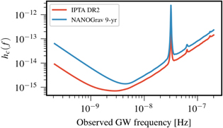
To quantify the improvement offered by the IPTA over NANOGrav-only data, we use the IPTA's second data release (Perera et al. 2019), DR2, and compare its sensitivity to that of the NANOGrav subset of the DR2 data set, i.e., the NANOGrav 9 yr data set (NG9; NANOGrav Collaboration et al. 2015). We estimate the sensitivity using hasasia (Hazboun et al. 2019a, 2019b), a software package that can compute the per-frequency sensitivity of any PTA given the white- and red-noise properties of the pulsars. We use the noise properties of the pulsars provided with the public DR2 data, but do not include intrinsic red noise because these parameters are highly covariant with a common process and would require a full GWB detection analysis for accurate calculation.
The per-frequency sensitivities of IPTA DR2 and NG9 are shown in Figure 7. IPTA DR2 is more sensitive across all frequencies than NG9. Consequently, IPTA DR2 achieves a total-signal significance that is a factor of 30 higher than NG9. This corresponds to a decrease in the fractional uncertainty on the GWB amplitude and spectral index by factors of 4 and 5.5, respectively. Note that these are only estimates because (as previously mentioned) no intrinsic red noise was accounted for in the sensitivity curves, which would have the effect of reducing each of the S/N values. However, given these estimates, an analysis of a combined IPTA data set offers the opportunity to detect a GWB and extract the underlying astrophysics of the source population at a faster pace and with higher significance than can be achieved with any individual PTA.
Figure 7. The sensitivity curve for IPTA DR2 and the NANOGrav 9 yr data set, which was one of the components going into the construction of DR2. These sensitivity curves were constructed using hasasia and only used the white-noise parameters released with IPTA DR2. The IPTA DR2 is more sensitive at all frequencies than the NANOGrav 9 yr data set.
Download figure:
Standard image High-resolution image
7. Conclusion
The recent NANOGrav evidence of a common-spectrum process is a tantalizing hint of the first signs of a GWB with growing significance in PTA data. As such, we have developed a road map for the next several years that includes three key PTA scientific milestones: (I) robust detection of the GWB through measuring HD-correlated timing delays across the PTA, (II) discriminating the origin of the GWB as being from either a population of SMBHBs or exotica, and (III) unveiling the demographic and dynamical properties of SMBHBs as encoded in the shape of the recovered GWB strain spectrum. All of these milestones could be achievable by the middle of this decade under conservative assumptions, and even sooner under the auspices of the IPTA.
This work has been carried out by the NANOGrav collaboration, which is part of the International Pulsar Timing Array. The NANOGrav project receives support from National Science Foundation (NSF) Physics Frontiers Center award number 1430284. This work made use of the Super Computing System (Spruce Knob) at West Virginia University (WVU), which are funded in part by the National Science Foundation EPSCoR Research Infrastructure Improvement Cooperative Agreement #1003907, the state of West Virginia (WVEPSCoR via the Higher Education Policy Commission), and WVU. Some of our models utilized the IllustrisTNG simulations public data release (http://www.tng-project.org/; Nelson et al. 2019) and sublink merger trees (Rodriguez-Gomez et al. 2015).
The Flatiron Institute is supported by the Simons Foundation. Pulsar research at UBC is supported by an NSERC Discovery Grant and by the Canadian Institute for Advanced Research. J.S. and M.V. acknowledge support from the JPL RTD program. S.B.S. acknowledges support for this work from NSF grants #1458952 and #1815664. S.B.S. is a CIFAR Azrieli Global Scholar in the Gravity and the Extreme Universe program. S.R.T. acknowledges support from NSF grant AST-#2007993 and a Dean's Faculty Fellowship from Vanderbilt University's College of Arts & Science. T.T.P. acknowledges support from the MTA-ELTE Extragalactic Astrophysics Research Group, funded by the Hungarian Academy of Sciences (Magyar Tudományos Akadémia), which was used during the development of this research. T.D. and M.T.L. acknowledge NSF AAG award number 2009468. Support for Dr. Cromartie was provided by NASA through the NASA Hubble Fellowship Program grant #HST-HF2-51453.001 awarded by the Space Telescope Science Institute, which is operated by the Association of Universities for Research in Astronomy, Inc., for NASA, under contract NAS5-26555. This work is supported in part by NASA under award number 80GSFC17M0002.
Software: ENTERPRISE (Ellis et al. 2019), enterprise_extensions (Taylor et al. 2018), hasasia (Hazboun et al. 2019a), libstempo (Vallisneri 2020), matplotlib (Hunter 2007), PTMCMC (Ellis & van Haasteren 2017).
Footnotes
- 43
But note that such a broadband primordial GWB signal with similar amplitude to the common-spectrum process found in the NANOGrav 12.5 yr analysis could be constrained at higher frequencies by ground-based GW interferometers and big bang nucleosynthesis (e.g., Kuroyanagi et al. 2021).