Electromagnetic Turbulence in the Electron Current Layer to Drive Magnetic Reconnection

Magnetic reconnection is a fundamental process in plasma that enables fast release of the magnetic field energy into plasma kinetic energies (Biskamp 2000; Yamada et al. 2010). The reconnection process is driven by the dissipation of the magnetic field around the x-line that breaks the field line connectivity. It has been suggested that plasma turbulence is responsible for the generation of the dissipation through wave–particle interactions in high energy environments (Davidson & Krall 1977). However, the generation mechanism of turbulence as well as the macroscopic description of the dissipation process remain unsolved.

High energy plasmas prevailing in space, astrophysics, and fusion environments are recognized as collisionless plasma where the Coulomb collision scales are much larger than typical spatiotemporal scales of the phenomena of interest. In such environments, the dissipation from the binary collisions is too weak to drive magnetic reconnection. Instead, plasma turbulence is expected to give rise to an effective collision through momentum exchange between the species and/or momentum transport across the flow shear layer. In fact, the reconnection current layer could be unstable to a variety of plasma instabilities (Fujimoto et al. 2011), since it is characterized by intense relative flow of electrons and ions that is significantly localized in space. Observations in the Earth's magnetosphere and laboratory experiments have also shown strong wave activities around the x-line, suggesting a link between turbulence and the reconnection process (Ji et al. 2008; Zhou et al. 2009). Full kinetic simulations in the three-dimensional (3D) system have provided evidence for the generation of intense turbulence in the electron layer that sensitively depends on the initial magnetic field configuration (Che et al. 2011; Daughton et al. 2011; Fujimoto & Sydora 2012; Roytershteyn et al. 2012). The present study focuses on the antiparallel and symmetric case, which is the most basic and fundamental configuration.

Macroscopic modeling of magnetic reconnection has been extensively examined in the magnetohydrodynamics (MHD) framework. Although the MHD model enables easy access to large-scale dynamics, the kinetic processes are not treated explicitly. The magnetic dissipation in MHD usually occurs from ad hoc resistivity that is artificially given. Although recent MHD simulations have suggested that the rate of reconnection is almost insensitive to the magnitude of the resistivity in a high Lundquist number regime (S ≳ 10⁵) (Bhattacharjee et al. 2009; Huang & Bhattacharjee 2010; Oishi et al. 2015), it has also been pointed out that numerical effects could not be excluded in the MHD simulations (Shimizu et al. 2017), where S denotes the Lundquist number. The resistive MHD model is based on the idea that the resistivity results from turbulence generating momentum exchange between electrons and ions. For the momentum exchange to arise, the turbulence forces on the ions and electrons must have the same magnitude and opposite sign (Miyamoto 1989). However, there is no guarantee that these forces dominate within the reconnection layer in the kinetic framework. In general, the momentum exchange results from drift-type instabilities excited by the relative velocity between the species (Coroniti & Eviatar 1977; Huba et al. 1977). These instabilities tend to be stabilized in the region of high plasma beta that is typical in the reconnection layer with the antiparallel and symmetric configuration. Instead, the high-beta current layer can be unstable to flow shear instabilities for laminar jets (Drazin & Reid 2004; Fujimoto & Sydora 2017). The shear modes generally result in the momentum transport across the shear layer, which leads to viscosity in the nonlinear stage. Indeed, the previous particle-in-cell (PIC) simulations have identified the dissipation in association with shear-type instabilities during reconnection (Che et al. 2011; Fujimoto & Sydora 2012). However, the macroscopic descriptions of the dissipation due to kinetic turbulence have been unrevealed in the reconnection diffusion region. Furthermore, the domain sizes of the previous kinetic simulations were too small, compared to realistic scales of the phenomena of interest. These uncertainties have motivated us to challenge the current MHD framework by means of large-scale kinetic simulations.

The simulation model employs the adaptive mesh refinement (AMR) to achieve efficient high-resolution kinetic simulation of multiscale processes, and the algorithm is massively parallelized on the modern supercomputer systems (Fujimoto 2011). The simulation is performed for a Harris-type current sheet (Harris 1962) with the magnetic field ${B}_{x}(z)=-{B}_{0}\tanh (z/\delta )$ and the number density $n(z)={n}_{0}{{\rm{sech}} }^{2}(z/\delta )+{n}_{b}{\tanh }^{2}(z/\delta )$, where δ is the half width of the current sheet and the subscript b indicates the background parameter. We choose δ = 0.5λ_i and n_b = 0.044n₀ with λ_i the ion inertia length based on n₀. The refinement criteria of the AMR are provided by the local electron Debye length λ_De and the electron flow velocity V_ey defined at the center of each computational cell. Each cell is subdivided when Δ_L ≥ 2.0λ_De or V_ey ≥ 2.0V_A are satisfied, otherwise the child cells are removed, if any, where Δ_L is the size of the square computational cells and V_A is the Alfvén velocity based on B₀ and n₀. The system boundaries are periodic in the x and y directions and the conducting wall in the z direction. The ion-to-electron mass ratio and velocity of light are m_i /m_e = 100 and c/V_A = 27, respectively, corresponding to ω_pe /ω_ce = 2.7, where ω_pe and ω_ce are the electron plasma frequency and cyclotron frequency based on n₀ and B₀, respectively. The temperature ratios are T_0i /T_0e = 5.0, T_bi /T_be = 1.0, and T_be /T_0e = 1.0, so that the background ions are colder than the plasma sheet ions. The system size is L_x × L_y × L_z = 81.9λ_i × 41.0λ_i × 81.9λ_i , which is entirely covered by base-level cells (coarsest cells) with ${{\rm{\Delta }}}_{{L}_{B}}=0.08{\lambda }_{i}$ and can be subdivided locally into finer cells up to the dynamic range level (finest level) with ${{\rm{\Delta }}}_{{L}_{D}}=0.02{\lambda }_{i}$. Therefore, the highest spatial resolution is 4096 × 2048 × 4096 and the maximum number of particles used is ∼ 4 × 10¹¹ for each species. The normalization parameters are m_i for mass, e for charge, λ_i for length, and V_A for velocity, unless otherwise noted. For comparison, additional 3D simulation with L_y = 10.2λ_i and a 2D simulation in the xz plane are conducted with the same initial setup.

Magnetic reconnection is initiated with a small perturbation to the magnetic field B_x and B_z (Fujimoto 2006), which produces the x-line at the center of the xz domain. The contributions of turbulence to the reconnection process are evaluated using the generalized Ohm's law averaged over the y-axis

$$\begin{eqnarray}\begin{array}{rcl}{\left\langle -{E}_{y}\right\rangle }_{\mathrm{an}} & = & \displaystyle \frac{1}{\left\langle {n}_{e}\right\rangle }\left\langle \delta {n}_{e}\delta {E}_{y}\right\rangle +\displaystyle \frac{1}{\left\langle {n}_{e}\right\rangle }{\left\langle \delta ({n}_{e}{{\boldsymbol{V}}}_{e})\times \delta {\boldsymbol{B}}\right\rangle }_{y}\\ & & +\displaystyle \frac{{m}_{e}}{e\left\langle {n}_{e}\right\rangle }{\left\{{\rm{\nabla }}\cdot \left\langle \delta \left({n}_{e}{{\boldsymbol{V}}}_{e}\right)\delta {{\boldsymbol{V}}}_{e}\right\rangle \right\}}_{y},\end{array}\end{eqnarray} \tag{ 1 }$$

where $A\equiv \left\langle A\right\rangle +\delta A$ for a variable A with $\left\langle A\right\rangle =\left(1/{L}_{y}\right){\int }_{0}^{{L}_{y}}A\,{dy}$, so that one can derive $\left\langle \delta A\right\rangle =0$. The first term on the right-hand side represents the contribution from electrostatic (ES) turbulence, while the second term gives the electromagnetic (EM) turbulence effects. The last term denotes the contribution from the inertia viscosity. The reconnection rate is calculated from the electric field E_y at the average x-line such that ${E}_{R}\equiv \left\langle -{E}_{y}\right\rangle /{V}_{{Au}}{B}_{u}$, where the subscript u denotes the instantaneous upstream values with ${V}_{{Au}}={B}_{u}/\sqrt{{\mu }_{0}{m}_{i}{n}_{u}}$ the Alfvén velocity, B_u the magnetic field magnitude, and n_u the plasma density.

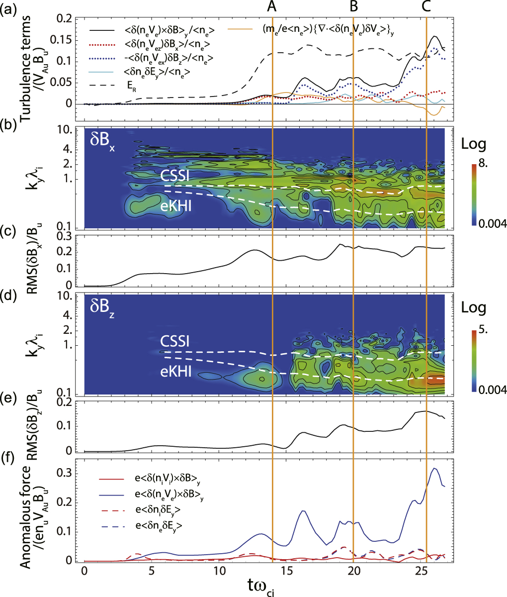
Figure 1 shows the time evolution of turbulence at the instantaneous x-line. After the onset of a fast reconnection at t ω_ci ≈ 13, formation and ejection of flux ropes are repeated in the electron current layer, which results in significant enhancement of the EM turbulence around the x-line (black solid curve in Figure 1(a)). On the other hand, the ES turbulence (water blue curve) and inertia viscosity (orange curve) terms are found to be much smaller than the EM turbulence term over most of the time period after t ω_ci ≈ 13. In particular, after t ω_ci ≈ 23, the EM turbulence is drastically increased and almost balances the reconnection electric field (dashed curve). It is found that this increase is mainly caused by the perturbation in B_z (blue dotted curve). The wave spectra in Figures 1(b) and (d) also show the intense wave activities after the onset of the fast reconnection. One can see that two kinds of wave modes dominate in the electron layer, peaking at ${k}_{y}{\lambda }_{i}^{* }\approx \sqrt{-{V}_{e0}/{V}_{i0}}$ (upper white dashed curves) in δ B_x and ${k}_{y}{\lambda }_{i}^{* }\approx 0.9$ (lower white dashed curves) in δ B_z , where ${\lambda }_{i}^{* }$ is the local ion inertia length and V_s0 is the peak flow velocity in the y direction of species s. The former mode is termed the current sheet shear instability (CSSI; Fujimoto & Sydora 2017), while the latter mode is identified as the electron Kelvin–Helmholtz instability (eKHI) oscillating in the xy plane (Fujimoto 2016). Both modes are driven by flow shear across the localized electron layer. Comparison between the EM turbulence (Figure 1(a)) and magnetic fluctuations (Figures 1(b)–(e)) indicates that the enhancement of the EM turbulence is mainly caused by the eKH waves through δ B_z . The process essentially differs from the previous ones (Che et al. 2011; Fujimoto & Sydora 2012; Roytershteyn et al. 2012; Price et al. 2016), where EM turbulence dominated in the yz plane, confined in the narrow electron layer, so that the turbulence intensity has been limited to a lower level.

Zoom In Zoom Out Reset image size

The enhancement of turbulence is also evident from the evolution of the current layer in Figure 2. At t ω_ci = 14.0, the electron layer formed around the x-line is almost laminar with weak perturbation in B_x and B_z (Figures 2(a), (d)). The contribution of the EM turbulence to the reconnection electric field is small at this stage (Figure 2(g)). Figure 3(a) shows the power spectrum density (PSD) of $\delta {E}_{y}\approx -{\left(\delta {{\boldsymbol{V}}}_{e}\times \delta {\boldsymbol{B}}\right)}_{y}$ along the average x-line. Because of the nonlinearity, the theoretical wavenumber of δ E_y is shifted to a higher value, by two times at most. Taking this effect into account, the expected spectral ranges for the eKHI and CSSI are indicated by blue and purple dashed lines, respectively. One can see that the activities of both the modes are low at this time. After a few flux rope ejections, the electron layer becomes more turbulent at t ω_ci = 20.0 (Figures 2(b), (e), (h), and 3(b)). In particular, the wave amplitudes in the ranges of the eKHI and CSSI are significantly intensified (Figure 3(b)). In association with the eKH waves, the flux rope has a structure along the y-axis (Figure 2(e)). The intermittent formation of the structured flux ropes results in further enhancement of the turbulence in the electron layer at t ω_ci = 25.4 (Figures 2(c), (f), (i), 3(c), and see also Figure 2's animation). At this time, the EM turbulence plays a primary role in supporting the reconnection electric field around the x-line (Figure 2(i)). As the turbulence evolves, a dominant x-line where the upstream magnetic flux ${\int }_{-{L}_{z}/2}^{{L}_{z}/2}| {B}_{x}| {dz}$ is minimum in each xz plane becomes discontinuous along the y-axis (Figures 2(d)–(f)), which implies that the reconnection process is fully 3D. The PSD profile in Figure 3(c) shows that the energy cascading is well established from macroscale to microscale, so that the current layer is sufficiently turbulent. It is interesting to note that the wave spectrum follows a large cascading rate with a −2.2 power law in the inertia range, unlike the Kolmogorov's −5/3 power law. This result is in contrast to that in the reference simulation with L_y = 10λ_i (gray curve) where the eKHI cannot be excited because of the small domain size. The difference in spectrum is possibly caused by the excitation of the eKHI in the larger simulation domain that introduces an additional turbulence energy source and changes the energy cascading process. The results suggest that the turbulence properties strongly depend on the simulation domain size.

Zoom In Zoom Out Reset image size

To model the dissipation process through the EM turbulence, we consider the force balance between electrons and ions. This is a new approach that is different from what has been used for strong guide-field cases (Biskamp 2000; Che et al. 2011), in which the EM turbulence term in (1) provided a good approximation of electron momentum transport. Note that the goal of the present study is to reveal the macroscopic description of the dissipation process through the turbulence. The dissipation locally occurs from the electron inertia effects (Vasyliunas 1975), while turbulence can cause overall momentum transfer (i.e., momentum exchange between the species and/or momentum transport across the current layer) that results in the overall dissipation in the turbulent current layer (Biskamp 2000; Yokoi & Hoshino 2011). Figure 1(f) compares the anomalous forces at the x-line on ions (red curves) and electrons (blue curves) from the EM (solid curves) and ES (dashed curves) turbulences. It is clearly shown that the EM turbulence mainly works on the electrons alone, while the ions are not significantly affected. The result implies that the EM turbulence hardly drives the momentum exchange between the species, which fails to produce the resistivity. In comparison, the forces from the ES turbulence are almost the same magnitude and have opposite signs between the electrons and ions. Thus, it works for the momentum exchange resulting in the resistivity. However, the ES turbulence is much weaker than the EM turbulence in the current simulation.

The eKHI is excited due to the electron flow shear across the electron current layer along the x-axis. The generation mechanism can be explained within the electron MHD framework (Bulanov et al. 1992). The evolution of δ B_z is provided by Faraday's law, ∂δ B_z /∂t ≈ − ∂δ E_y /∂x. We assume here that unperturbed B_z is negligibly small and plasma is incompressible. Under this condition, δ E_y may be approximated by the electron inertia term as $\delta {E}_{y}\sim -({m}_{e}/e)\left\langle {V}_{{ey}}\right\rangle ^{\prime} \,\delta {V}_{{ex}}$, leading to

$$\begin{eqnarray}&&\displaystyle \frac{\partial \delta {B}_{z}}{\partial t}\sim \displaystyle \frac{{m}_{e}}{e}\left\langle {V}_{{ey}}\right\rangle ^{\prime\prime} \,\delta {V}_{{ex}}.\end{eqnarray} \tag{ 2 }$$

Here, $\left\langle {V}_{{ey}}\right\rangle ^{\prime} =\partial \left\langle {V}_{{ey}}\right\rangle /\partial x$, $\left\langle {V}_{{ey}}\right\rangle ^{\prime\prime} ={\partial }^{2}\left\langle {V}_{{ey}}\right\rangle /\partial {x}^{2}$, and ∂δ V_ex /∂x ≈ 0 is assumed at the x-line. Assuming stationary growing waves with the growth time τ_g ∼ γ⁻¹, one can estimate $\delta {B}_{z}\sim \left({m}_{e}/e\right){\tau }_{g}\left\langle {V}_{{ey}}\right\rangle ^{\prime\prime} \,\delta {V}_{{ex}}$, where γ is the growth rate of the eKHI. The contribution of the EM turbulence to the reconnection field can be estimated as ${\left\langle -{E}_{y}\right\rangle }_{\mathrm{an}}\,\approx -\left\langle \delta {V}_{{ex}}\delta {B}_{z}\right\rangle \,\sim -\left({m}_{e}/e\right){\tau }_{g}\left\langle {V}_{{ey}}\right\rangle ^{\prime\prime} \left\langle \delta {V}_{{ex}}^{2}\right\rangle$. Normalized to the upstream quantities, and with an approximation of $\left\langle {V}_{{ey}}\right\rangle \approx -\left\langle {J}_{y}\right\rangle /{{en}}_{e}$, the anomalous reconnection field can be written in the form

$$\begin{eqnarray}&&{\left\langle -{E}_{y}\right\rangle }_{\mathrm{an}}^{* }\sim {\mu }_{\mathrm{an}}^{* }\displaystyle \frac{{\partial }^{2}{\left\langle {J}_{y}\right\rangle }^{* }}{\partial {x}^{* 2}},\end{eqnarray} \tag{ 3 }$$

where the asterisks denote the renormalized quantities, and ${\mu }_{\mathrm{an}}^{* }={\tau }_{g}^{* }{{\lambda }_{e}^{* }}^{2}{\left\langle \delta {V}_{{ex}}^{2}\right\rangle }^{* }$ is identified as the anomalous viscosity generated by the eKH waves. The growth rate of the eKHI can be approximated by γ* ∼ γ/ω_ci,u ≈ 1 from the linear analysis (Fujimoto 2016), so that ${\tau }_{g}^{* }\sim {\gamma }^{* -1}\approx 1$, where ω_ci,u = eB_u /m_i .

Figure 4 evaluates the theoretical prediction in Equation (3), assuming ${\left\langle -{E}_{y}\right\rangle }_{\mathrm{an}}\approx -\left\langle \delta ({n}_{e}{V}_{{ex}})\delta {B}_{z}\right\rangle /\left\langle {n}_{e}\right\rangle$ in the vertical axis. The large error bars along the horizontal direction result from large spatial fluctuations in ${\partial }^{2}\left\langle {J}_{y}\right\rangle /\partial {x}^{2}$, in particular, when the turbulence intensity is large. We have averaged the values along the x-axis to reduce the statistical noise to obtain a smooth function. Regardless of the large fluctuation, there is a clear tendency that the anomalous reconnection field balances the viscous effect driven by the eKH waves through the anomalous momentum transport. The simulation results demonstrate that the anomalous viscosity, rather than the anomalous resistivity, plays a primary role in generating the dissipation to drive reconnection.

Zoom In Zoom Out Reset image size

We have shown that the eKHI plays a primary role in driving intense EM turbulence leading to the dissipation in the reconnection current layer. We find that the ions hardly react to the turbulence, indicating that the turbulence does not cause significant momentum exchange between electrons and ions resulting in the resistivity. Instead, the dissipation is mainly generated by viscosity associated with electron momentum transport across the current layer. The present results suggest a fundamental modification of the current MHD models using the resistivity to drive magnetic reconnection.

The EM turbulence also affects the energy conversion process in the reconnection current layer. Figure 5 (solid curve) shows a z profile of the electron temperature $\left\langle {T}_{e}\right\rangle$ through the x-line, where T_e = (T_ex + T_ey + T_ez )/3 with ${T}_{{ej}}=({m}_{e}/{n}_{e}){\int }_{-\infty }^{\infty }{\left({v}_{j}-{V}_{{ej}}\right)}^{2}{f}_{e}({\boldsymbol{v}}){d}^{3}{\boldsymbol{v}}$ for j = x, y, and z. It is found that the electrons are strongly heated in the current layer much more than the cases of 2D simulation (dotted curve) and 3D simulation with smaller domain size (dashed curve). Furthermore, the current sheet width is apparently increased with the domain size, because of larger diffusivity due to more intense EM turbulence in the larger domain. Consequently, the electron thermal energy in the current layer for the case of L_y = 41λ_i becomes more than double the case of the 2D simulation. The strong electron heating and current sheet broadening are consistent with recent results from laboratory experiments, where the electron heating cannot be explained in 2D PIC simulations (Yamada et al. 2014).

Zoom In Zoom Out Reset image size

The immediate impact of the present results should be crucial to understand the substorm process in the Earth's magnetosphere, where antiparallel and symmetric reconnection occurring in the magnetotail can trigger the global magnetospheric energy release. Most global MHD simulation models have employed an ad hoc artificial resistivity to drive reconnection. However, it is known that the global behavior of the magnetosphere sensitively depends on the resistivity model (Raeder et al. 2001; Kuznetsova et al. 2007). The modification of the MHD models by replacing the resistive force ( ∝ η J ) with the viscous force ( ∝ − μ∇² J ) is likely to give significant changes in the global dynamics and contribute to better modeling of the substorm dynamics as well as the reconnection process.

The simulations were carried out by the K computer at the RIKEN Advanced Institute for Computational Science through the HPCI Research project (hp140129, hp150123). The data analyses were partly performed on analysis servers at Center for Computational Astrophysics (CfCA), NAOJ. This research was supported by the National Natural Science Foundation of China under grant Nos. 41874189 and 41821003, and the Natural Science and Engineering Research Council of Canada.