Source Depth of Three-minute Umbral Oscillations

Oscillations of intensity and velocity are common in sunspots, in both umbrae and penumbrae. At the chromospheric level, the oscillation periods are generally shorter than three minutes in umbrae (Bogdan & Judge 2006), and gradually increase with the distance from the sunspot center (Nagashima et al. 2007). It is generally accepted that sunspot oscillations are the slow magnetohydrodynamic (MHD) waves propagating along magnetic field lines (Centeno et al. 2006; Jess et al. 2013). Multi-line spectral observations have indicated that the waves propagate upwardly inside umbrae (Felipe et al. 2010).

Although it is known that the slow MHD waves propagate along the magnetic fields, sunspot oscillations are often observed to propagate across the magnetic fields. The most well-known phenomenon is running penumbral waves (Zirin & Stein 1972). These are usually observed as horizontal propagating patterns with fast speed in penumbral regions. It is widely accepted that they are the apparent waves caused by the slow MHD waves propagating along different inclined penumbral magnetic field lines (Bloomfield et al. 2007; Löhner-Böttcher & Bello González 2015; Madsen et al. 2015). The difference in the inclination among the penumbral magnetic field lines produces the difference in the path length, and, hence, the time lag at the detection layer that increases with the distance from the sunspot center. As a result, we observe successive arrivals of the slow MHD waves, which appear as the apparent horizontal propagation. This interpretation can explain both the horizontal propagations and period increase with distance from the sunspot center (Jess et al. 2013).

Interestingly, the horizontally propagating waves are found even in umbrae. Rouppe van der Voort et al. (2003) found spreading bright arcs from Ca ii H filtergram data, which represent the horizontally propagating pronounced intensity oscillations known as umbral flashes. Velocity oscillations often form concentric ripple-like patterns crossing the umbrae transversely (Zhao et al. 2015; Cho et al. 2019). Even more complicated shapes such as spiral wave patterns also exhibit the horizontal propagation inside umbrae (Sych & Nakariakov 2014; Su et al. 2016; Felipe et al. 2019; Kang et al. 2019). These horizontally propagating patterns inside umbrae cannot be explained by the time lag due to the magnetic field inclination unlike the case of the running penumbral waves because their inclination angle is very close to zero or 180°.

The horizontally propagating pattern of oscillations in umbrae can be explained if the source of wave excitation is located at a point inside the interior. In the high plasma β environment of the interior, such a source excites fast MHD waves that propagate in all the directions (Zhugzhda & Dzhalilov 1982, 1984). When they reach the photosphere, the time of arrival depends on the path and hence varies with the position of the photosphere. This introduces the time lag in the photosphere, which appears as the horizontally propagating pattern. Theoretical studies have indicated that the fast MHD waves can generate the slow MHD waves in the photosphere via the fast-to-slow mode conversion (Cally 2001). If this explanation is feasible, then the propagation aspect of the horizontally propagating patterns must be affected by the internal structures of sunspots where the fast MHD waves passed and especially the depth of the wave source.

In the present work, we infer the depth of the wave source from the observed horizontally propagating patterns of oscillations. This work is based on our recent study (Cho et al. 2019, hereafter Paper I) on the excitation events of umbral oscillations. Among them, we choose five ripple-like patterns that show concentric shapes and propagate horizontally. We build an internal model of a sunspot to calculate the ray path of the fast MHD waves. Then the source depth is estimated from the model fitting of the propagating distance of a Doppler pattern determined as a function of time in each event. The obtained values of source depth are compared to previous reports, and we discuss the results in association with the origin of the three-minute umbral oscillations.

We observed umbral oscillations around 21:00 UT on 2017 June 15 using the Fast Imaging Solar Spectrograph (FISS; Chae et al. 2013). The target was located in the leading sunspot of AR 12663 (25'', 205'') which was near the solar disk center. This observation data set is the same as the one used in Paper I.

The FISS provides four-dimensional (two spatial, spectral, and temporal dimensions) data in two bands simultaneously. In this observation, the pair of the Fe i 5435 Å band and the Na i D2 5890 band was chosen. We utilize only the Fe i 5435 Å line data that has the advantage in line-of-sight velocity measurements inside sunspots because of the zero Landé g factor (g = 0). The FISS observed 40'' × 13'' field of view at every 13 s. The details of the basic data processing were described by Chae et al. (2013). We inferred the line-of-sight Doppler velocity at all the positions from the FISS Fe i 5435 Å spectra using the Gaussian core fitting. We also exploit the speckle-reconstructed TiO 7057 Å broadband filter images (Cao et al. 2010) to check the photospheric features of our region of interest. The TiO images were used as the reference for the alignment of the FISS data. For magnetic field information, we use Near-InfraRed Imaging Spectropolarimeter (NIRIS) data (Cao et al. 2012).

We identified five ripple patterns from the three-minute filtered Doppler velocity movie. The identified ripple patterns constitute the event 1 and 2 in Paper I. The event 1 and 2 has a peak of power at 3.2 minute, and 4.1 minute period, respectively. Both events had more than half of the oscillation power between 2 and 4 minute period. From the wavelet filtering data through the passband of periods between 2 and 4 minutes (Torrence & Compo 1998), we found simple concentric shaped ripple patterns.

We determined the oscillation center of each ripple and traced its propagation. The oscillation center was identified with the position of the peak Doppler signal at the very early phase as in Paper I. By applying the azimuthal averaging, we obtained the Doppler velocity as a function of time t and distance from the oscillation center x. The pattern of azimuthally averaged Doppler velocity v_D(x, t) was modeled by the function

$$\begin{eqnarray}&&{v}_{D}(x,t)={a}_{0}(t)\sin [{a}_{1}(t)x+{a}_{2}(t)]+{a}_{3}(t).\end{eqnarray} \tag{ 1 }$$

The coefficients a₀(t), a₁(t), a₂(t), and a₃(t) were determined from the model fit in the distance range of 05–4'' at each time. The values of a₁(t), and a₂(t) were then used to determine the position of peak blueshift ${x}_{b}(t)=[3\pi /2-{a}_{2}(t)]/{a}_{1}(t)$ at each time. For the redshift cases, we used a formula ${x}_{r}(t)=[\pi /2-{a}_{2}(t)]/{a}_{1}(t)$.

We adopted a model of wave propagation that takes into account several processes (see Figure 1). We suppose a point-like event of wave generation takes place much below the umbral photosphere. The point source is in an environment of high plasma β, so the generated waves propagate mainly as the fast MHD waves. The propagation speed of the fast MHD waves v_f is

$$\begin{eqnarray}&&{v}_{f}={\left(\displaystyle \frac{1}{2}({c}_{s}^{2}+{v}_{{\rm{A}}}^{2})+\sqrt{{\left({c}_{s}^{2}+{v}_{{\rm{A}}}^{2}\right)}^{2}-4{c}_{s}^{2}{v}_{{\rm{A}}}^{2}{\cos }^{2}\theta }\right)}^{1/2}\end{eqnarray} \tag{ 2 }$$

where c_s is sound speed, v_A is Alfvén speed, and θ is the angle between the propagating direction and the magnetic field lines. We assumed that magnetic fields in the umbra are vertical even below the photosphere. A part of the fast MHD waves propagate upward and reach the β ≃ 1 layer where the sound speed is roughly equal to the Alfvén speed, and where a part of fast MHD waves are converted to slow MHD waves (Cally 2001; Schunker & Cally 2006). These slow MHD waves propagate the same distance along the vertical magnetic field lines. Thus, the time differences at the β ≃ 1 layer among different field lines are consequently preserved in the slow MHD wave mode. As a result, we come to observe the apparent horizontal propagation of waves at the Fe i 5435 Å line formation height of about 280 km (Chae et al. 2017).

We adopt the umbral E model of Maltby et al. (1986) to obtain the sound speed at each height. To determine the Alfvén speed, we need magnetic field strength as a function of height. We used the mean magnetic field strength of 2480 G inferred from the Milne-Eddington inverted Fe i 1.56 μm NIRIS data. The formation height of that line in sunspot umbra is about 90 km (Bruls et al. 1991), and we employed the vertical gradient of −1 G km⁻¹ (Borrero & Ichimoto 2011). By comparing the c_s and v_A, we calculate the height where plasma β is unity (Figure 1(b)). The result is consistent with our picture that the deeper region shows high plasma β and the upper region shows low plasma β. The β ≃ 1 layer is found to be about 13 km above the photospheric layer.

In reality, the fast MHD waves are refracted because of the variation of the phase velocity with heights. We calculate the refracted ray path of the fast MHD waves and the time of arrival on the β ≃ 1 layer using the eikonal method (Weinberg 1962; Moradi & Cally 2008). Given dispersion relation D, the relations between position x, wavevector k, time t, and frequency ω for the wave propagation of the same phase are governed by following equations:

$$\begin{eqnarray}&&\displaystyle \frac{d{\boldsymbol{x}}}{d\tau }=\displaystyle \frac{\partial D}{\partial {\boldsymbol{k}}}\end{eqnarray} \tag{ 3 }$$

$$\begin{eqnarray}&&\displaystyle \frac{d{\boldsymbol{k}}}{d\tau }=-\displaystyle \frac{\partial D}{\partial {\boldsymbol{x}}}\end{eqnarray} \tag{ 4 }$$

$$\begin{eqnarray}&&\displaystyle \frac{{dt}}{d\tau }=-\displaystyle \frac{\partial D}{\partial \omega }\end{eqnarray} \tag{ 5 }$$

$$\begin{eqnarray}&&\displaystyle \frac{d\omega }{d\tau }=-\displaystyle \frac{\partial D}{\partial \tau }.\end{eqnarray} \tag{ 6 }$$

In case of the fast MHD waves, the dispersion relation is given by

$$\begin{eqnarray}&&D={\omega }^{4}-({c}_{s}^{2}+{v}_{{\rm{A}}}^{2}){k}^{2}{\omega }^{2}+{c}_{s}^{2}{v}_{{\rm{A}}}^{2}{k}^{2}{k}_{z}^{2}=0.\end{eqnarray} \tag{ 7 }$$

We set the oscillation frequency ω to be 0.035 s⁻¹, which corresponds to about 3 minutes. In fact, our results do not depend on the frequency because we do not take into account gravity (Kalkofen et al. 1994; Chae & Goode 2015). As it is not a dispersive medium, phase speed of the fast MHD waves does not depend on the frequency (see Equation (2)). The ray paths of the fast MHD waves are calculated from a point with a given depth for several initial angles (Figure 1(a)). As a result, we obtain the distance from the oscillation center and duration until the fast MHD waves reach the β ≃ 1 layer and then we are able to calculate the horizontal position of the apparent wave as a function of time.

Interestingly, the speed of apparent horizontal propagation strongly depends on the depth of the source. The animation associated with Figure 1 clearly shows that a shallower source yields a slower apparent speed, while a deeper source yields a faster apparent speed. This is because ray paths of the waves that originated from a deeper source are not much different from each other. So, the fast MHD waves arrive almost at the same time, and it looks like that the apparent waves propagate quickly. We can explain the variation of the propagating speed with the distance from the oscillation center in a similar way. We estimate the depth by fitting the observed distance of the peak blueshift x_b(t) by the one calculated with the model of wave propagation.

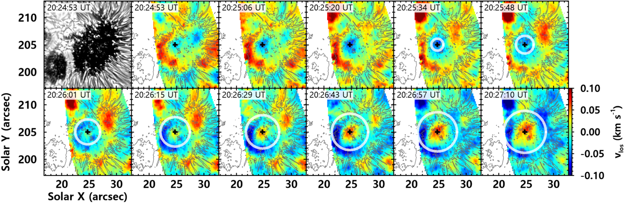
Figure 2 shows the time series of the Doppler velocity maps showing the propagation of ripple 1. We found that a blueshift ripple emerged from the oscillation center near the umbral center; then it propagated radially. The associated animation clearly shows that the selected five ripples propagated outward with concentric circle shape.

We measured the distances of ripple 1 from the oscillation center (Figure 3). The pattern of azimuthally averaged Doppler velocity oscillated with an amplitude of about 0.05 km s⁻¹ and propagated outward. The fitting results obviously show that the pattern can be well described by a sinusoidal function of distance. We will describe ripple 1 in detail. From the fitting, we find that the amplitude of Doppler velocity range from 0.023 to 0.11 km s⁻¹ with a mean of about 0.048 km s⁻¹. The spatial wavelength was determined to range from 42 (3000 km) to 11'' (7800 km) with the mean value of 68 (4900 km). The ripple moved away from the oscillation center as we expected. Moreover, the distance between two successive ripples decreased with time, which implies that the speed decreased with the propagation distance. The determined speed was initially 27 km s⁻¹ and decreased to about 13 km s⁻¹, which is much faster than the slow MHD waves at the detection layer.

Zoom In Zoom Out Reset image size

The dashed lines in Figure 4 show the distance of the ripple as a function of time calculated using our model of wave propagation in each case of the source depths. In each time–distance plot, the horizontal propagation speed can be inferred from the slope of the curve. It usually starts with a high value and decreases with time, and approaches an asymptotic value. This asymptotic speed, as well as the average speed, depends on the model and increases with the source depth of the model.

Zoom In Zoom Out Reset image size

The data (distances and times) of all the ripples marked in the figure by the symbols closely match the models presented in thick solid curves. The data are very similar to the models, particularly in the trend of the decreasing velocity with the time or the propagation distance from the oscillation center. Based on our results, we conclude that the depth of the oscillation sources ranges from about 1400 to 1800 km with a mean value of about 1600 km below the photosphere.

We observed the horizontally propagating ripples in a sunspot umbra. These cannot be explained by slow MHD waves only, because slow MHD waves propagate vertically along magnetic fields. We attempted to interpret their horizontal propagations as the apparent ones caused by the time lag. It is assumed that the time lag is the result of the different arrival times of the fast MHD waves below the plasma β ≃ 1 layer. We constructed a model based on this scenario and fitted the observational data. The observational results were successfully reproduced by our calculations with a depth of about 1600 km. The decrease of the propagating speed with distance is also adequately explained by our model calculations.

We expect that there are two major sources of error in calculating the source depth. First, the measurement error of the positions of ripples can affect the result. This is also closely related to the determination of the oscillation center. We posit that the measurement error is less than 1'', which corresponds to about 1000 km variation of depth. The second source is an inaccurate model. We deduced the variation of the sound speed and Alfvén speed with depth from the sunspot atmospheric model and the magnetic field information. The most ambiguous information is the vertical gradient of the magnetic field strength. In the high β regime, however, the fast MHD waves are not significantly affected by the magnetic field strength. We have tested several cases of magnetic field strength, then concluded that there might be an error of about a few hundred km in the depth estimation. Thus it is reasonable to state that the wave source is roughly located between 1000 and 2000 km depth. To obtain more accurate depth, and explain the frequency dependent behavior of the waves (Zhao et al. 2016), it is necessary to examine the effects of gravity on the wave propagation.

Our result is in agreement with previous studies (Figure 5). Meyer et al. (1974) theoretically studied the instability of the sunspot model. As a result, it was demonstrated that overstable oscillation may occur in the top 2000 km of sunspots with the parallel motion to the magnetic field. From the HMI Dopplergram data, Zhao et al. (2015) found fast-moving waves with speeds of about 45 km s⁻¹ using the time–distance cross-correlation method. They conjectured that a disturbance occurring at about 5000 km under the sunspot surface from the MHD sunspot model and the ray-path approximation with magnetic fields. Felipe & Khomenko (2017) performed MHD numerical simulations to confirm the dependence of the source depth. They concluded that the measured horizontal fast-moving waves are consistent with waves generated between about 1000 and 5000 km beneath the sunspot photosphere. Analyzing the result of the 3D radiative MHD simulations, Kitiashvili et al. (2019) identified that most of the wave sources are concentrated below 1000 km in the pore-like magnetic structure. Kang et al. (2019) argued that 1600 km of source depth is required to explain the spiral wave patterns in sunspots using a simplified wave propagation model. Our estimate, the source depth of about 1600 km, is fairly consistent with these results.

Zoom In Zoom Out Reset image size

Our study contributes to the understanding of the generation of the umbral three-minute oscillations. Our result suggests that the origin of the umbral three-minute oscillations is located below the photosphere as a point source. It supports the internal excitation as the origin of the umbral oscillations. Paper I found the association of the oscillation center and the umbra dots in the photosphere. Considering that umbra dots are regarded as the signature of the magnetoconvection, we can posit the shape of a magnetoconvection cell. The average size of an umbral dot is less than 1'' (≃700 km). Taking into account the source depth close to 2'' (≃1500 km), we imagine that the cell of the magnetoconvection may be vertically elongated. This vertical elongation seems to be reasonable in the umbral environment permeated by strong vertical magnetic field lines. Previous studies based on MHD simulations exhibited such vertically elongated convection cells with comparable physical size (Schüssler & Vögler 2006; Rempel et al. 2009).

It would be worthwhile to examine the azimuthal dependence of the horizontal propagation. We only used the azimuthally averaged Doppler velocity in this study. It is known that the asymmetric behavior arises from the difference in the time legs, which is affected by a different path, magnetic field inclination, flows, and temperature variation (e.g., Kosovichev & Duvall 1997). Therefore, the relevant studies will provide information about the magnetoconvection inside sunspot, and eventually the internal structure of sunspots.

We greatly appreciate the referee's constructive comments. This work was supported by the National Research Foundation of Korea (NRF-2017R1A2B4004466) and the Korea Astronomy and Space Science Institute under the R&D program (project No. 2020-1-850-07) supervised by the Ministry of Science and ICT.