


Abstract
The extended jets of the microquasar SS 433 have been observed in optical, radio, X-ray, and recently very-high-energy γ-rays by High Altitude Water Cerenkov (HAWC). The detection of HAWC γ-rays with energies as great as 25 TeV motivates searches for high-energy γ-ray counterparts in the Fermi-Large Area Telescope (LAT) data in the 100 MeV–300 GeV band. In this paper, we report on the first joint analysis of Fermi-LAT and HAWC observations to study the spectrum and location of γ-ray emission from SS 433. Our analysis finds common emission sites of GeV-to-TeV γ-rays inside the eastern and western lobes of SS 433. The total flux above 1 GeV is  in both lobes. The γ-ray spectrum in the eastern lobe is consistent with inverse Compton emission by an electron population that is accelerated by jets. To explain both the GeV and TeV flux, the electrons need to have a soft intrinsic energy spectrum, or undergo a quick cooling process due to synchrotron radiation in a magnetized environment.
Export citation and abstract BibTeX RIS
1. Introduction
SS 433 is a microquasar in the supernova remnant W50 (see Margon 1984; Fabrika 2004 and references therein). It is likely composed of a ∼20 M⊙ black hole orbiting a ∼30 M⊙ supergiant companion with a 13.1 day period. The exotic system is located at a distance of 5.5 kpc (Blundell & Bowler 2004; see discussions about other distance measures in, e.g., Marshall et al. 2013) and about 2° below the Galactic plane. It produces two remarkable jets with kinetic power Lkin ∼ 1039 erg s−1. The jets are heavily loaded with baryons and move at a speed of 0.26c while precessing with a period of 162 days. The angle between the jets and the axis is ∼20°. Other periods are measured but the dynamics is poorly understood (Eikenberry et al. 2001).
Extended X-ray jets are observed on the eastern and western sides (in Galactic coordinates) of SS 433, as shown by the white contours in Figure 1 (Safi-Harb & Ögelman 1997). They interact with and distort the shell of the W50 nebula (Watson et al. 1983; Gregory et al. 1996). which is shown by the gray contours. A set of emission regions, denoted as e1, e2, and e3 centered at 24', 35' and 60' east of SS 433, and w1 and w2 centered at 18' and 31' west of SS 433. have been investigated in detail (Safi-Harb & Ögelman 1997). A bright knot is seen in soft X-rays at e2 (Safi-Harb & Ögelman 1997; Brinkmann et al. 2007), and emission from e1, e2 and w1, w2 is observed in hard X-rays (Safi-Harb & Petre 1999; Moldowan et al. 2005). The X-ray emission can be explained by synchrotron radiation of ∼100–200 TeV electrons in a ∼10 μG magnetic field.

Figure 1. SS 433/W50 region in the 10.5 yr Fermi-LAT data between 100 MeV and 300 GeV (left) and from joint analysis of the Fermi-LAT data and the 1017 days HAWC data (right) in Galactic coordinates. Left: the color scale indicates the statistical significance for a point source following an E−2 spectrum as a function of position. The figure is a test statistic map after fitting γ-rays from known sources in the 4FGL catalog. Right: the background includes the 4FGL sources and J1913+0515 in the GeV band, and MGRO J1908+06 in the TeV band. The color scale indicates the improvement of the total likelihood of the region of interest (ROI) by a test point source that follows a log parabola spectrum in each 0 1 × 01 grid inside the purple squares. The maps are smoothed by a Gaussian interpolation. The γ-ray hotspots revealed by joint analysis are inside the lobes and close to hard X-ray emission sites. For comparison, the locations of SS 433, the jet termination regions e1, e2, e3, w1, and w2 observed in the X-ray data are indicated as orange crosses. FL8Y J1913.3+0515 is marked by a white cross. The white and gray contours show the X-ray at ∼0.9–2 keV (Safi-Harb & Ögelman 1997) and radio emission at 4.85 GHz (Gregory et al. 1996). For a SS 433 distance of 5.5 kpc, 30' corresponds to 50 pc.
Download figure:
Standard image High-resolution imageVery-high-energy (VHE) γ-ray emission has recently been detected from the SS 433 lobes by the High Altitude Water Cerenkov (HAWC) observatory (HAWC Collaboration et al. 2018). In a data set based on 1017 days of measurements, photons with energies of at least 25 TeV are observed. The TeV hotspots are located close to e1, e2, and w1, with spatially unresolved emission profiles. The flux can be explained by the inverse Compton emission of the same electron population whose synchrotron emission is observed by X-ray telescopes. On the other hand, 40–80 hr observations with the Major Atmospheric Gamma Imaging Cerenkov telescopes and High Energy Spectroscopic System (H.E.S.S.) report no evidence of γ-ray emission between a few hundred GeV and a few TeV from the jet termination regions, or from the central binary (MAGIC Collaboration et al. 2018). A similar upper limit is reported by the Very Energetic Radiation Imaging Telescope Array System (VERITAS; Kar & VERITAS Collaboration 2017).
Searches (Bordas et al. 2015; Rasul et al. 2019; Sun et al. 2019; Xing et al. 2019) have been made for a GeV counterpart in the data observed by the Fermi Large Area Telescope (LAT) (Atwood et al. 2009). Analysis of LAT data in this region faces two complications. A point source FL8Y J1913.3+0515 from the preliminary LAT 8 yr point source list4 (FL8Y) is tagged as possibly associated with W50. It is no longer a source in the 4FGL catalog due to different emission models (The Fermi-LAT Collaboration 2019). Different conclusions about detection of SS 433 have been reached depending on whether this source is included in the background model. In addition, analysis of the emission profile and spectrum of the SS 433 region is heavily impacted by the nearby pulsar PSR J1907+0602 (4FGL J1907.9+0602), which is not suppressed via selection on the rotational phase in the abovementioned works. Due to these difficulties, whether the jets of SS 433 shine at GeV energies is unknown.
Since the source is marginally significant in γ-rays yet close to the bright Galactic plane, it is difficult to study solely with the GeV or the TeV measurements. Here we jointly analyze an ROI surrounding SS 433 observed by LAT and HAWC. A simultaneous fit to the 100 MeV–100 TeV data directly addresses the question of whether γ-ray emission over six decades can be produced by a common cosmic-ray population inside the SS 433 lobes. We explain the methods in Section 2, present the results of the LAT analysis in Section 3.1 and that of the joint analysis in Sections 3.2 and 3.3. We discuss immediate implications of this analysis in Section 4.
2. Methods
Our analysis uses 10.5 yr of Fermi-LAT data and 1017 days of HAWC data. Details on the LAT and HAWC analyses, as well as background sources in each band, are presented in Appendices A and B. The setup of a joint analysis of the LAT and HAWC data based on the 3ML framework (Vianello et al. 2015) is presented in Appendix C. Here we describe the procedure for the joint analysis.
We first build a source model to describe the broadband γ-ray emission of SS 433. Three types of models are considered.
- 1.γ-rays follow a power-law spectrum,
 .
. - 2.γ-rays follow a log parabola spectrum,.
- 3.Electrons are injected with a rate, where γe = Ee/me c2 is the Lorentz factor of an electron. They up-scatter the cosmic microwave background (CMB) and infrared photons in W50 to γ-rays through the inverse Compton process, and produce synchrotron emission in a magnetic field B.


Models I and II are simple descriptions of γ-ray spectral shapes. Model III is physically motivated. The cooling time of VHE electrons,  kyr, is much less than the source age,
  (Fabrika 2004). In order to take into account the effects of cooling, we solve a transport equation for each set of parameter values. Details about the cooled electron spectrum can be found in Appendix D. Once a steady-state cosmic-ray spectrum is obtained, the γ-ray flux is calculated using the radiative functions of the naima package (Khangulyan et al. 2014; Zabalza 2015).
The models are then converted into data space and compared to observations through the joint analysis framework (see Appendix C). Since the GeV and TeV observations are carried out independently, a total log likelihood is evaluated by summing the log likelihoods from the GeV and TeV analyses. The total likelihood is then maximized by adjusting model parameters to obtain the best-fit source model. Finally, the likelihood test statistic (TS) of a target source is computed as twice the difference of the log likelihoods of the data given the models with and without the source.
3. Results
3.1. LAT Analysis Results
Here we present results from the LAT-only analysis. The method is detailed in Appendix A. The main difference between our analysis and previous works is that we use a data set for which the PSR J1907+0602 is gated off, that is, the arrival times of photons are phase-folded, and the photons that arrive during the pulsar's pulse peak are removed (see J. Li et al. 2019, in preparation for details). Throughout the work we use the 4FGL catalog and the corresponding diffuse emission models to model background sources.
The significance of the residual γ-ray excess from the SS 433/W50 region in the LAT data between 100 MeV and 300 GeV is shown in the left panel of Figure 1. The most statistically significant excess is near the location of FL8Y J1913.3+0515. We call this excess J1913+0515 to differentiate it from FL8Y J1913.3+0515. J1913+0515 is at the boundary of W50, well outside the extended X-ray jets. When describing the spectral energy distribution (SED) with a power-law function, we obtain  ,
,  , and αγ = 2.4. The best-fit location is very close but slightly different from the location listed in the FL8Y catalog. The test statistic of the source is TS = 32.8 using a regular likelihood and TS = 25.7 using a weighted likelihood (The Fermi-LAT Collaboration 2019) that takes into account estimated systematic uncertainties in the diffuse emission models. As the results obtained by the two methods are similar, we use a regular (i.e., unweighted) likelihood in the rest of our analyses.
A sub-threshold (TS < 25) excess is evident at the northeastern side of J1913+0515. Because it is spatially close to the TeV excess in the eastern lobe, we refer to it as the "eastern hotspot." It is not significant in the LAT data and has TS = 5.0 when J1913+0515 is included in the background model. The excess is due to several high-energy photons at ∼20–50 GeV, as shown by the SED in the top panel of Figure 2.
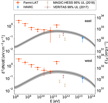
Figure 2. The best-fit γ-ray spectra in the eastern and western lobes obtained by joint analysis assuming that γ-rays are produced by an electron population (Model III). The parameters and TS of the model are listed in Table 1. The gray shaded area indicates the 68% statistical uncertainty from a fit that varies the normalization. For comparison, we show the SED from the LAT-only analysis (Section 3.1, red markers), HAWC-only analysis (Appendix B, HAWC Collaboration et al. 2018; blue markers), upper limits on γ-rays from nearby regions by VERITAS (Kar & VERITAS Collaboration 2017) and HESS (MAGIC Collaboration et al. 2018) (gray markers). For the LAT data points, 95% upper limits are shown when TS < 4, otherwise 1σ error bars are shown. Since IACT limits are converted from integral limits, they do not have horizontal error bars. We find that the γ-ray emission in the eastern lobe can be explained as the inverse Compton emission by a cooled electron population.
Download figure:
Standard image High-resolution imageIn the western lobe, a sub-threshold excess is found between w1 and w2 (which we refer to as the "western hotspot" below). The excess region partially overlaps with the X-ray jets and touches the boundary of W50. We find a TS of 16.1 for the western hotspot when adding it to the baseline model. Its spectrum can be described by a power law of index 2.3, as shown in the bottom panel of Figure 2.
When including the potential sources in the baseline model simultaneously, we obtain TS ∼ 5 and TS ∼ 10 for the eastern and western hotspots, respectively. The fit results are summarized in Table 2 in Appendix A. Neither of the "hotspots" is statistically significant in the LAT observations but they are evident in the joint analysis, as will be shown in Section 3.3.
3.2. J1913+0515 and the TeV Emission
To investigate whether J1913+0515 and the TeV emission in the eastern lobe share a common origin, we test two ways of combining the GeV and TeV hotspots.
First, we replace J1913+0515 and the TeV excess with a single source centered between them and assume that it has a power-law spectrum. The joint fit has six free parameters in total, including spectral index, flux normalization, extension of MGRO J1908+06, and flux normalization and location (R.A., decl.) of the test source. Due to the low statistics, it is difficult to fit the spectral index and the flux normalization of the test source simultaneously. We thus fix the index as αγ = 2.2 and vary only the prefactor. Following Wilks (1938) theorem and Chernoff & Lehmann (1954), we calculate the probability of the TS using a chi-square distribution with three degrees of freedom, which is the difference in dimensionality of the models when including and excluding the test source. We then evaluate the corresponding number of standard deviations for this confidence level for a Gaussian distribution.
We find TS = 32.1 for the test source, which includes 16.9 from a comparison with the LAT data, and 15.2 from a comparison with the HAWC data. The TS corresponds to 5.0σ standard deviation.
Alternatively, we assume that the sources share a spectrum but differ in emission sites. The fit results in TS = 30.3 from GeV data and TS = 23.8 from TeV data. The total significance increases to 6.4σ, despite the two extra degrees of freedom due to the additional emission site. In general, we find that the LAT TS of the common source increases and the HAWC TS decreases when the test source is moved toward J1913+0515, and the trend is reversed when the test source is moved toward the VHE hotspot. Such a trend, along with the considerable difference in the statistical significances of the models with one and two source locations, suggest that J1913+0515 is unlikely to be a counterpart of the TeV hotspot in the eastern lobe.
3.3. Joint Analysis Results
Motivated by results from the last section, we perform a joint analysis of LAT and HAWC data with J1913+0515 added to the background. The parameters and TS of the models are summarized in Table 1. For rectangular areas with Δ l = 05 and Δ b = 05 that cover the e1, e2 and w1, w2 regions, we compute the TS of a test source at every 01 × 01 grid point assuming a log parabola spectrum (Model II). The scanned regions are enclosed by the purple squares in Figure 1. A log parabola spectrum is chosen because it describes the LAT SED and the HAWC flux better than a power-law spectrum. We take Model II with αγ = 1.8, βγ = 0.05, Eγ,piv = 60 GeV but have verified that alternative log parabola shapes (for example with αγ = 1.7, βγ = 0.05, Eγ,piv = 5 GeV), lead to similar results. We leave the normalization Kγ as a free parameter. For background sources, we free the normalization and index of J1913+0515, the normalization and extension of MGRO J1908+06, and fix parameters of the rest of sources in the ROI. The map of TS for the best source positions considered is shown in the right panel of Figure 1. We find that when including the TeV data, the eastern hotspot becomes significant, and can be resolved from J1913+0515.
To directly check whether the GeV-to-TeV emission can be explained as inverse Compton emission of the same electron population, we perform a joint fit with the electron model (Model III). We fix the parameters in both lobes as αe = 1.9, B = 20 μG, and Ee,max = 1 PeV and free the normalizations of the electron spectra. These parameters and their values are motivated by the fit to the broadband multi-wavelength data in HAWC Collaboration et al. (2018). We do not scan the parameter space for these parameters, but note that the electron energy needs to be higher than 150 TeV to produce the measured 20 TeV photons. In general higher Ee,max leads to better fits. The best-fit model has a TS of 40 when fitting both lobes simultaneously. With six free parameters including the two normalizations and the coordinates of the two hotspots, the TS corresponds to a significance of 5σ for a two-sided Gaussian distribution. The fit results using all three models are listed in Table 1. They are all significant, suggesting that the GeV-to-TeV γ-rays can be explained by common sources inside the SS 433 lobes.
Table 1. Fit Results
| Source | Position | TS (Individual) | Modela | Significance | ||
|---|---|---|---|---|---|---|
| (R.A., Decl. in degree) | LAT | HAWC | Individual | Total | ||
| Eastern hotspot | (288.56, 4.95) | 1.9 | 21.6 | I | 4.2σ | 5.5σ |
| Western hotspot | (287.58, 5.01) | 8.9 | 12.1 | I | 3.9σ | |
| Eastern hotspot | (288.56, 4.95) | 4.3 | 21.7 | II | 4.4σ | 5.4σ |
| Western hotspot | (287.58, 5.01) | 4.6 | 12.4 | II | 3.4σ | |
| Eastern hotspot | (288.56, 4.95) | 3.3 | 19.9 | III | 4.1σ | 5.0σ |
| Western hotspot | (287.58, 5.01) | 5.2 | 10.8 | III | 3.3σ | |
Note.
aFor particular models, certain parameters are held constant. They include: Model I, Epiv = 875.753 MeV, αγ,W = 2.2, αγ,E = 2.1; Model II, αγ = 1.8, βγ = 0.05, Eγ,piv = 60 GeV; Model III, αe = 1.9, B = 20 μG, and Ee,max = 1 PeV. R.A. and decl. are for epoch J2000. See the text for additional details.Download table as: ASCIITypeset image
The SED is shown in Figure 2. For comparison, we also show the SED obtained from the LAT-only analysis, the upper limits (UL) on nearby γ-ray emission by imaging air Cerenkov telescopes (IACTs), and the flux at the pivot energy Epiv = 20 TeV from the HAWC-only analysis. We find that the γ-ray flux and the cosmic-ray injection rates of the east and the west hotspots are very similar. To explain both the GeV and TeV flux, a soft electron spectrum dN/dE ∼ E−3 is needed. This can be achieved by a relatively inefficient acceleration (Blandford & Eichler 1987) or by cooling of electrons as suggested by HAWC Collaboration et al. (2018). The flux at GeV energies is higher than that predicted by HAWC Collaboration et al. (2018). This suggests that a far-infrared (FIR) background needs to be present (whose energy density is discussed in Appendix D).
The best-fit models predict a sub-TeV γ-ray flux that is higher than the upper limits from IACTs. The upper limits are based on observations of e2, w2 (H.E.S.S.), and w1 (VERITAS) with small angular extents defined by X-ray observations, so they do not necessarily apply to the actual source locations in these models.
The western source is less significant in all cases, which could be due to confusion by Galactic diffuse emission and with MGRO J1908+06. The location of the γ-ray emission site in the western lobe is less clear. Like the eastern side, the localized GeV emission could be a combination of emission inside the lobe and at the boundary of W50, though more statistics is needed to verify this scenario.
4. Discussion
Because of its proximity and exotic structure, SS 433 has been one of the most observed Galactic high-energy sources for over 40 yr. Nonetheless, no consensus has been reached about what happens inside the SS 433/W50 complex. The detection of multiple tens of TeV photons from the object confirms the existence of particles at extreme energies, but deepens the question of why lower-energy γ-rays have not been observed. By jointly analyzing an ROI measured by both the Fermi-LAT and the HAWC Observatory, we find common sites of GeV and TeV γ-ray emission inside the SS 433 lobes. The SED is consistent with inverse Compton emission of an electron population accelerated by the jets but quickly cooled due to synchrotron radiation in a magnetized environment. We use a data set that suppresses emission by a nearby pulsar that highly impacts previous analyses. Our joint analysis concludes that the GeV point source J1913+0515 located at the boundary of W50 is an unlikely counterpart to the TeV emission. This addresses the dilemma encountered by Xing et al. (2019), Sun et al. (2019), and Rasul et al. (2019).
This is the first joint ROI analysis across γ-ray observatories, to our knowledge. Using a framework built on individual data analysis toolkits from γ-ray observatories, we have shown that such an approach is feasible. The joint analysis is designed to study shared properties of sources of γ-rays over a very broad spectrum. It maximizes the usage of data, including sub-threshold information, and is more powerful than simply combining results from each experiment. Future data from HAWC, especially with refined angular resolutions (HAWC Collaboration et al. 2019), will help improve the understanding of γ-ray emission from the western lobe. Future observations by IACTs, as well as by X-ray and radio telescopes, at the revised source locations will help further constrain the emission models.
The GeV–TeV spectrum can be explained as inverse Compton scattering by X-ray synchrotron-emitting ∼100 TeV electrons. Three scenarios can be entertained to account for the acceleration. The first is to invoke direct, diffusive shock acceleration of the electrons at the termination shocks of the precessing jets launched by the accretion disk. If the post-shock field strength is ∼10 μG then acceleration to these energies is possible, though only a small electron power ∼1034 erg s−1 is needed to account for the γ-rays. Second, ∼5 PeV protons may also be shock-accelerated. Their primary radiative loss could be due to Bethe–Heitler pair production on ∼2 eV optical photons from SS 433 with a cross section of a few millibarn. Maximum electron or positron energies ∼100 TeV are just possible. However, in order to account for the γ-ray power, a proton power ∼1038 erg s−1 is necessary. The third possibility is that a hitherto unobserved, ultrarelativistic, electromagnetic jet is formed by the spinning black hole. Such a jet can create an EMF ∼ 100(Ljet/1039 erg s−1)1/2 PV that suffices to accelerate the emitting particles. Finally, if the gas density in the lobes is high ( ), pion production can also make a contribution to the γ-ray flux. High-energy neutrinos would be produced simultaneously and could be measured by IceCube (IceCube Collaboration et al. 2019).
Future multi-messenger observations of the γ-ray emission regions have the potential to discriminate between these scenarios.
The Fermi LAT Collaboration acknowledges generous ongoing support from a number of agencies and institutes that have supported both the development and the operation of the LAT as well as scientific data analysis. These include the National Aeronautics and Space Administration and the Department of Energy in the United States, the Commissariat à l'Energie Atomique and the Centre National de la Recherche Scientifique/Institut National de Physique Nucléaire et de Physique des Particules in France, the Agenzia Spaziale Italiana and the Istituto Nazionale di Fisica Nucleare in Italy, the Ministry of Education, Culture, Sports, Science and Technology (MEXT), High Energy Accelerator Research Organization (KEK), and Japan Aerospace Exploration Agency (JAXA) in Japan, and the K. A. Wallenberg Foundation, the Swedish Research Council, and the Swedish National Space Board in Sweden.
Additional support for science analysis during the operations phase is gratefully acknowledged from the Istituto Nazionale di Astrofisica in Italy and the Centre National d'Études Spatiales in France. This work was performed in part under DOE Contract DE-AC02-76SF00515.
We thank Henrike Fleischhack, Colas Riviére, and Giacomo Vianello for their help with the usage of the 3ML and HAWC-HAL packages.
Appendix A: Fermi-LAT Analysis
We analyze 10.5 yr of Pass 8 data5 taken between 2008 August 4 15:43:36 UTC and 2019 January 28 00:00:00 UTC using version 0.17.4 of fermipy6 and version ScienceTools-11-04-00 of Fermitools.7 We define the ROI as the 15° × 15° region in Galactic coordinates centered at SS 433 (l = 39.69, b = −2.24). γ-ray events with energies between 100 MeV and 300 GeV are selected. Other event selection criteria include a 90° zenith cut and a filter expression of "DATA_QUAL > 0 && LAT_CONFIG == 1" which are standard quality criteria recommended by the Fermi Science Support Center. We use the P8R2_SOURCE event selection, and the corresponding P8R2_SOURCE_V6 LAT instrument response functions. Unlike previous works analyzing the SS 433 region (Rasul et al. 2019; Sun et al. 2019; Xing et al. 2019), here we use the latest LAT 8 yr Point Source Catalog (The Fermi-LAT Collaboration 2019), together with the corresponding Galactic diffuse model gll_iem_v07.fits and the isotropic diffuse model. The 4FGL catalog and the updated diffuse emission model turn out to considerably impact the analysis of 100–300 MeV photons in this region, comparing to the FL8Y catalog.
As the nearby pulsar PSR J1907+0602 is very bright in the GeV band, we use the same method from J. Li et al. (2019, in preparation) to suppress the pulsar emission. The same pulsar ephemeris is adopted in pulsar gating, which amounts to 44% of the observing time. The exposure is scaled accordingly.
There are 33 4FGL sources within 5° of SS 433 and 61 4FGL sources within 8°. The baseline ROI analysis is performed using the fermipy.job sub-package fermipy-analyze-roi. The optimized model is referred to as "baseline model."
A significance map of the residual γ-ray excess is shown in the left panel of Figure 1. The color scale corresponds to the square root of the TS when there is a new point source at a given location, in addition to known sources from the 4FGL catalog, the Galactic diffuse emission and the isotropic diffuse emission. The test point source is assumed to have an E−2 spectrum and the TS is evaluated for each location on a grid with 01 × 01 spacing.
After setting up the baseline model, we add J1913+0515, the eastern and western hotspots, to the background model and refit the new model to the data. The new model is refit to the data using GTAnalysis.optimize, which fits sources in order of their fluxes. The fit returns TS values of 26.1, 5.0, and 9.6 for the three candidate sources, respectively. We also tested an alternative fitting method, where we fixed the parameters of background sources to their best-fit values, and vary only the normalization of new sources using GTAnalysis.fit. This approach returned TS values of 28.0, 4.9, and 10.4 for the three. Since the difference of the results from the two fitting methods is minor while the latter is much more efficient in computation time, we use the second approach to calculate the LAT likelihood in a joint analysis. The fit results are summarized in Table 2.
Table 2. Significance of the Candidate Sources in the LAT Data
| Note | Source | Position (R.A., Decl. in degree, J2000) | 1σ Uncertainty (in degree) | TS |
|---|---|---|---|---|
| Fit individually | J1913+0515 | (288.30, 5.24) | 0.06 | 32.8 |
| With J1913 | eastern hotspot | (288.56, 4.95) | 0.27 | 5.0 |
| Fit individually | western hotspot | (288.53, 4.93) | 0.13 | 16.1 |
| Fit two sources simultaneously | J1913+0515 | (288.31, 5.24) | 0.06 | 28.4 |
| western hotspot | (287.58, 5.01) | 0.16 | 9.7 | |
| Fit three sources simultaneously | J1913+0515 | (288.31, 5.24) | 0.06 | 26.1 |
| eastern hotspot | (288.56, 4.95) | 0.33 | 5.0 | |
| western hotspot | (287.58, 5.01) | 0.17 | 9.6 | |
Download table as: ASCIITypeset image
Although MGRO J1908+06 is one of the brightest TeV sources, an extended source at its location is not significant in the LAT data. We thus do not include it in our background model.
The data points for the SED were obtained by binning the spectrum with 2 bins per decade in energy and performing a likelihood analysis in each energy bin.
Appendix B: HAWC Analysis
In the TeV band, we analyze the public data8
from the HAWC Observatory (HAWC Collaboration et al. 2018). The data set contains 1017 days of γ-ray events collected between 2014 November 26 and 2017 December 20. The reconstruction of the arrival direction of primary γ-rays is based on the relative arrival times of photoelectron hits detected by the photomultipliers inside the water Cerenkov detectors. (This kind of reconstruction is referred to as the nhit method.) Angular resolution from the nhit analysis ranges from around 1° below 1 TeV to <02 above 10 TeV.
We adopt the same ROI as in HAWC Collaboration et al. (2018), which is defined to be a semicircular region with a radius of 25 centered on the position of MGRO J1908+06 (as shown in Extended Data Figure 1 of HAWC Collaboration et al. 2018). By masking the sources close to the Galactic plane, the contamination from the Galactic diffuse emission is significantly reduced.
Three sources remain in the ROI: MGRO J1908+06, the eastern and the western hotspots in the SS 433 lobes. Following HAWC Collaboration et al. (2018), we use the electron diffusion model to describe the spatial morphology of MGRO J1908+06. Other spatial models with Gaussian and power-law radial profiles lead to similar results.
Unlike the analysis in HAWC Collaboration et al. (2018), which is based on the HAWC analysis framework AERIE, here we redo the analysis using the HAWC Accelerated Likelihood (HAL) framework. HAL provides faster convolution with the detector response functions, which is needed for the joint analysis in our work. We have confirmed that the two analysis frameworks lead to results that are consistent at the 1% level.
Appendix C: Joint Analysis
The workflow of a joint analysis is diagrammed in Figure 3. The joint analysis is implemented in the Multi-Mission Maximum Likelihood framework (3ML; Vianello et al. 2015).9 3ML is a data analysis architecture that converts emission models for an ROI into data spaces for specified instrument(s), and compares the model predictions to the corresponding data based on the likelihood formalism. The Fermi-LAT module of the package provides a wrapper of fermipy (Wood et al. 2017) and the Fermi Science Tools.10 The HAWC module links to the HAWC analysis tools including the Accelerated Likelihood (HAL) framework.11

Figure 3. Diagram of the workflow of a joint analysis of the Fermi-LAT and HAWC data around SS 433. The source model describes the γ-ray emission of the potential sources and may depend on the parent particle types, injection spectra, source locations, and magnetic field strength. The background model is composed of dozens of 4FGL sources, the diffuse emission models in the GeV band, and MGRO J1908+06 in the TeV band. The models are passed to analysis pipelines for the two data sets, converted to data space, and compared to data separately. The total likelihood is maximized to obtain the best-fit model.
Download figure:
Standard image High-resolution image
Since an ROI analysis is not implemented in 3ML, we use fermipy to perform a "baseline" analysis externally (see Appendix A) and use that as a starting point for 3ML analysis. Meanwhile, the source model and a model of MGRO J1908+06 are passed to the HAWC plugin (see Appendix B). In this way the contribution of background sources is taken into account properly.
Appendix D: Radiative Cooling of Electrons
The cooling of relativistic electrons in the lobes of SS 433 can be described by a transport equation:

where  is the energy loss rate due to inverse Compton and synchrotron emission. σT is the Thomson cross section. Ne and Qe are the spectrum and injection rate of electrons, respectively. uB = B2/(8π) and
  are the energy density of magnetic field and the CMB. We also adopt a FIR background at 20 K with
  motivated by the dust emission in the solar neighborhood (Vernetto & Lipari 2016). Background photons with higher energies are not important due to the Klein–Nishina effect. Due to its much lower energy density, the synchrotron radio emission of W50 and the lobes is not expected to contribute significantly to the cooling of electrons or production of high-energy γ-rays. In Equation (1) we have ignored the diffusion of electrons, as it is a slower process than cooling for TeV electrons, and also because doing so saves computing time. Assuming that electrons are injected with a simple power-law spectrum constantly over time,
  , the solution of Equation (1) can be written as

where ![${t}_{\min }=\max [0,t-{\nu }^{-1}({\gamma }_{e}^{-1}-{\gamma }_{e,\max }^{-1})]$](https://content.cld.iop.org/journals/2041-8205/889/1/L5/revision1/apjlab62b8ieqn14.gif) is the earliest time that an electron with γe can be injected and still not cooled after time t, and γe,max is the maximum electron energy.
is the earliest time that an electron with γe can be injected and still not cooled after time t, and γe,max is the maximum electron energy.
Footnotes
- 4
- 5
- 6
- 7
- 8
- 9
- 10
- 11