


Abstract
Planets orbiting within the habitable zones of M stars are prime targets for future observations, which motivates a greater understanding of how tidal locking can affect planetary habitability. In this Letter we will consider the effect of tidal locking on limit cycling between snowball and warm climate states, which has been suggested could occur for rapidly rotating planets in the outer regions of the habitable zone with low CO2 outgassing rates. Here, we use a 3D Global Climate Model that calculates silicate-weathering to show that tidally locked planets with an active carbon cycle will not experience limit cycling between warm and snowball states. Instead, they smoothly settle into "Eyeball" states with a small unglaciated substellar region. The size of this unglaciated region depends on the stellar irradiation, the CO2 outgassing rate, and the continental configuration. Furthermore, we argue that a tidally locked habitable zone planet cannot stay in a snowball state for a geologically significant time. This may be beneficial to the survival of complex life on tidally locked planets orbiting the outer edge of their stars, but might also make it less likely for complex life to arise.
Export citation and abstract BibTeX RIS
1. Introduction
Planets orbiting M stars are likely to be the most common type of terrestrial planets in the galaxy. A number of them have already been found in the habitable zone of their stars (TRAPPIST-1e, Proxima Centauri b, and LHS 1140b; Anglada-Escudé et al. 2016; Dittmann et al. 2017; Gillon et al. 2017). There has been a large amount of work on whether they could be habitable, which remains a topic of debate (e.g., Joshi et al. 1997; Segura et al. 2005; Merlis & Schneider 2010; Kite et al. 2011; Pierrehumbert 2011; Wordsworth et al. 2011; Leconte et al. 2013; Menou 2013; Yang et al. 2013, 2014; Hu & Yang 2014, 2014; Barnes et al. 2016; Kopparapu et al. 2016; Turbet et al. 2016; Wolf 2017; Abbot et al. 2018; Chen et al. 2018; Lewis et al. 2018; Meadows et al. 2018; Yang et al. 2019). The habitable zone of M stars lies at a small orbital distance since they are dimmer than G stars. Because of this, planets orbiting within their habitable zones are particularly likely to become tidally locked to their stars, in a 1:1 spin:orbit configuration (Kasting et al. 1993). Planets orbiting larger K and G stars can also become tidally locked (Barnes 2017), although it is less likely. A tidally locked configuration may affect a planet's potential for habitability in different ways, such as forcing a large temperature contrast between the substellar and antistellar regions that could lead to atmospheric collapse on the night side if the atmospheric pressure is too low.
One issue of interest in this Letter is that rapidly rotating terrestrial planets orbiting G stars are subject to snowball (global glaciation) events associated with bifurcations and climate hysteresis as a result of the ice-albedo feedback (Budyko 1969; Sellers 1969). Snowball events are even believed to have occurred in Earth history (Kirschvink 1992; Hoffman et al. 1998, 2017). The tidally locked orbital configuration, however, suppresses the possibility of these snowball bifurcations, regardless of the stellar spectrum (Checlair et al. 2017). This is due to the strong increase in stellar irradiation as the substellar point is approached on tidally locked planets. The M-star spectrum also peaks at a wavelength where the albedos of snow and ice are lower, which reduces the amount of hysteresis associated with the snowball bifurcation, although it does not prevent the bifurcation for rapidly rotating planets (Joshi & Haberle 2012; Shields et al. 2013).
The silicate-weathering feedback is an important regulator of surface temperature on terrestrial planets (Walker et al. 1981). It involves the balance between the outgassing of CO2 from the interior and the removal of CO2 from the atmosphere by continental weathering, which depends strongly on temperature and precipitation. If the surface temperature decreases, continental weathering slows, allowing atmospheric CO2 to build up and bringing the temperature back up. This feedback allows a planet to maintain habitable conditions within the habitable zone (Kasting et al. 1993). However, if the CO2 outgassing and received stellar flux are too low, a planet would be subject to climate cycles between snowball and warm climate states (Kadoya & Tajika 2014; Menou 2015; Abbot 2016; Batalha et al. 2016; Haqq-Misra et al. 2016; Paradise & Menou 2017). Haqq-Misra et al. (2016) suggested that climate limit cycles may not occur for planets orbiting M stars because of the reduced ice-albedo feedback (Joshi & Haberle 2012; Shields et al. 2013). However, they used a 1D climate model so they could not consider the effects of tidal locking.
In this Letter we use a 3D Global Climate Model (GCM) that calculates weathering to show that tidally locked planets in the habitable zone with an active carbon cycle cannot stay in a snowball state and will not be subject to climate cycling due to the lack of hysteresis in their climate, regardless of stellar type. They will instead settle into stable "Eyeball" states (Pierrehumbert 2010a) with open ocean in the substellar region. The size of this unglaciated region gradually increases as the stellar irradiation or the CO2 outgassing rate increase. We perform our simulations with a G-star spectrum, to show that these conclusions hold even if the ice-albedo feedback is strong.
2. Methods
We use Planet Simulator (PlaSim; Fraedrich et al. 2005), an intermediate-complexity 3D-GCM. We simulate and compare both a rapidly rotating and a tidally locked configuration. In both cases, we use the same PlaSim configuration as Checlair et al. (2017), with 32 latitudes, 64 longitudes, and 10 vertical layers. In order to isolate the effects of tidal locking, we perform simulations with a G-star spectrum here. One important aspect of PlaSim that we will later refer to is that the sea ice scheme assumes that a gridbox is either completely covered with sea ice or completely ice-free, so that partial sea ice coverage of a gridbox is not allowed.
We modified PlaSim following the method of Paradise & Menou (2017) to calculate the weathering rate at every model gridbox and timestep for a fixed amount of atmospheric CO2. This method is similar to that of Edson et al. (2012). We use the weathering rate formulation used by Menou (2015), which is based on a parameterization of Earth's continental silicate-weathering in the absence of plants and is motivated by observations and laboratory measurements:
where Ts is the surface temperature, pCO2,⊕ is the pre-industrial pCO2 of 330 μbar, and W⊕ is the weathering rate at Ts = 288 K. kact is related to the chemical activation energy of the weathering reaction and is set to 0.09, and krun is a runoff efficiency factor set to 0.045, which helps account for changes in precipitation. β is the dependence on pCO2, and is set to 0.5 (Kump et al. 2000; Pierrehumbert 2010b; Menou 2015). As in Paradise & Menou (2017), we evaluate Equation (1) at each land grid cell if the surface temperature is above 273.15 K every 6 hr of model simulation. These local rates are then averaged over the planet to obtain globally averaged weathering rates.
We run a total of 24 simulations with fixed values of CO2 pressure ranging from 0.1 to 4.6 × 10⁵ μbars. Each simulation is run for 100 yr, or until thermal equilibrium is reached. We compute the globally averaged weathering rate for each of these fixed CO2 pressures at equilibrium using the method laid out in Section 2. This gives us weathering as a function of CO2 (W(CO2)). Note that the snowball bifurcation allows W(CO2) to be multivalued. We evolve CO2 in time using the differential equation

for a chosen outgassing rate (V). In this work we assume Earth's outgassing rate is V⊕ = 7 bars Gyr−1 as in Menou (2015).
3. Results
3.1. Rapidly Rotating Planet
First, we reproduce the results of Paradise & Menou (2017), who demonstrated that CO2 limit cycles occur for an Earth-like rapidly rotating planet at a stellar irradiation of 1300 Wm−2. We plot cycles for an outgassing rate of V = 0.09  in Figure 1, and obtain cycles similar to those of Paradise & Menou (2017, see their Figure 3).
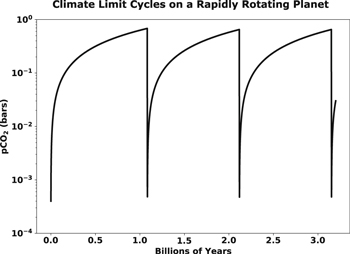
Figure 1. Rapidly rotating Earth-like planets with low outgassing rates are subject to climate limit cycles between warm and snowball states. This figure shows the CO2 cycles between warm and snowball climate states for a rapidly rotating Earth-like planet. Since weathering is near zero in the snowball state, the CO2 slowly builds up until a critical point at which the planet deglaciates. Warm continent is then exposed, allowing weathering, and the CO2 rapidly decreases until the snowball state is entered again. Outgassing rate is set to V = 0.09 V⊕. Stellar irradiation is fixed at 1300 Wm−2.
Download figure:
Standard image High-resolution imageParadise & Menou (2017) used an outgassing rate an order of magnitude lower than ours, yet the periods of our cycles unexpectedly differ only slightly. This is due to different assumptions made in obtaining our normalizing factors and to a conversion factor bug in their work that was fixed for this Letter. These differences do not change the qualitative nature of their results. In addition to this, the timescales found in both of our results are highly dependent on our simplified weathering prescription and should therefore be taken only as qualitative results.
Next, we vary the outgassing rate in Equation (2) to search for the value at which a climate cycle first appears. We summarize our results in Figure 2. When no cycle occurs, the planet is in a stable state and we plot the equilibrium CO2 (red solid line, warm state). When cycles occur, the planet is in a nonlinear limit cycle, and we plot the maximum and minimum CO2 pressures for that cycle (red and blue dashed lines, warm and snowball states). Outgassing rates higher than 0.87 bars Gyr−1 (0.12 V⊕) do not allow for climate cycles. This is roughly an order of magnitude higher than what Paradise & Menou (2017) found and can be attributed to the conversion factor bug mentioned above. We note that the critical outgassing value at a stellar irradiation of 1300 Wm−2 is still one order of magnitude smaller than Earth's outgassing.
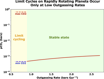
Figure 2. Outgassing rates must be lower than a critical value to allow for climate limit cycles between warm and snowball states on rapidly rotating Earth-like planets. This figure shows that for a stellar irradiation of 1300 Wm−2, the outgassing rate must be lower than the critical value of 0.87 bars Gyr−1 (0.12 V⊕) to allow for climate cycles. The dashed lines represent the upper (red dashed) and lower (blue dashed) limits between which CO2 oscillates as part of a nonlinear limit cycle when the outgassing rate is lower than the critical value. The solid line represents climates where the outgassing rate is too high for limit cycles to occur so that CO2 equilibrates to a fixed value with the planet in a stable warm state.
Download figure:
Standard image High-resolution image3.2. Tidally Locked Planet
We begin by reproducing the results of Checlair et al. (2017), who showed that habitable tidally locked planets do not exhibit a snowball bifurcation, but here we vary CO2 rather than stellar irradiation. We refer the reader to Checlair et al. (2017, Figure 7) for a bifurcation diagram of a rapidly rotating planet exhibiting the snowball bifurcation. Specifically, we compute the globally averaged equilibrium surface temperature for a planet initialized from a warm (globally ice-free) and a cold (globally ice-covered) state for a variety of CO2 pressures with a stellar irradiation of 1100 Wm−2 and a G-star spectrum (Figure 3). We find similar results to Checlair et al. (2017), with a single continuum of states smeared over about 5 K in global mean temperature and no bifurcation. This compares to a difference in temperature of 40–60 K between the warm and cold states when there is a bifurcation (Checlair et al. 2017). Any simulation started within the continuum of states equilibrates to the same state it started in. The continuum of states is an artifact of PlaSim's simple sea ice scheme where a grid cell can only be fully ice-covered or fully ice-free. We refer the reader to Checlair et al. (2017, appendix) for further analysis on the origin of the continuum of states and here simply note that it is unrelated to the snowball bifurcation. In a separate work (Checlair et al. 2019), we used ROCKE-3D, a sophisticated 3D-GCM that allows for partially ice-covered grid cells (Way et al. 2017) to reproduce these results for a tidally locked aquaplanet and found no continuum of states. We repeated these calculations for other stellar irradiations and found similar results. However, we note that we are never able to reach a fully glaciated state in a warm start configuration and a fully ice-free state in a cold start configuration for the same value of irradiation. The reason for this is that the partially glaciated state is stable over an extremely large range of radiative forcing and the PlaSim radiation scheme becomes significantly less accurate for CO2 values greater than ∼1 bar.
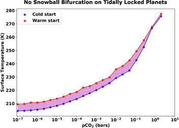
Figure 3. Tidally locked planets do not exhibit a snowball bifurcation. Planets initialized from both an ice-free (red) and an ice-covered (blue) state equilibrate to the same final continuum of states (purple). Stellar irradiation is fixed at 1100 Wm−2.
Download figure:
Standard image High-resolution imageTo investigate whether climate cycles can occur on tidally locked planets, we proceed with the same method used in our rapidly rotating case (Section 3.1). As Figure 4 shows, the planet equilibrates to a fixed value of CO2 for all outgassing rates and no cycles occur. Note that this is true even for extremely low CO2 outgassing rates, even three orders of magnitude lower than Earth's. The gap between the two curves (purple shaded region) is again due to the continuum of states that results from PlaSim's sea ice scheme.

Figure 4. Tidally locked planets do not go through climate limit cycles. As the outgassing rate is increased, the equilibrium CO2 pressure (A) and surface temperature (B) increase. This corresponds to an "Eyeball planet" with a substellar unglaciated region gradually increasing in size. This is a result of tidally locked planets lacking the snowball bifurcation. Stellar irradiation is fixed at 1100 Wm−2. The purple shaded region represents a continuum of states. Note that we consider extremely low CO2 outgassing rates.
Download figure:
Standard image High-resolution imageInstead of cycling between warm and snowball states, tidally locked planets settle into an "Eyeball" state with open ocean in the substellar region (Pierrehumbert 2010a). This is shown in Figure 5, where we map equilibrated annual-mean surface temperature and weathering rate for a tidally locked planet at an equilibrium outgassing rate of 1.1 × 10⁻³ bars Gyr−1, or 1.66 × 10⁻⁴ V⊕. Figure 5 suggests that the size of the open ocean region will be strongly dependent on the continental configuration. For a low CO2 outgassing rate, the climate adjusts so that the temperature is above freezing and weathering occurs in only a small region of land. If there is land closer to the substellar point, then the open ocean region will be smaller. Small increases in temperature cause large increases in weathering rate (Equation (1)), so the climate can exist in a very similar state for a large range of CO2 outgassing rates.

Figure 5. Example equilibrium state of a tidally locked planet at the outer edge of the habitable zone. The planet is in an Eyeball state with an unglaciated region centered at the substellar point. This figure shows maps of the equilibrated annual-mean surface temperature (top) and weathering rate (bottom) of a tidally locked planet at a very low equilibrium outgassing rate of 1.1 × 10⁻³ bars Gyr−1 (1.66 × 10⁻⁴ V⊕). The unglaciated region expands just enough for the temperature to be high enough in a small region of land that weathering there can balance this low CO2 outgassing rate. Stellar irradiation is fixed at 1100 Wm−2. The horizontal axis is longitude and the vertical axis is latitude.
Download figure:
Standard image High-resolution image
The position of the continents affects the weathering rate. To investigate this effect, we moved the substellar point from over the Pacific ocean (our default case) to over the African continent. We reproduced Figure 4 for these cases and found that although our qualitative results remained the same, the equilibrium surface temperatures and the CO2 pressures reached for each outgassing rate vary as a function of substellar point location. Given that a planet will always move toward weathering-outgassing equilibrium, sea ice must retreat until enough land is exposed for weathering to match outgassing. The distance between the substellar point and land therefore sets an upper limit on the amount of open ocean a tidally locked planet can have. Proximity of land to the substellar point on habitable tidally locked planets is therefore a dominant factor in determining equilibrium sea ice extent for a given outgassing rate.
4. Discussion
The most important outcome of this work is that tidally locked planets will not experience climate limit cycles. This is in contrast to rapidly rotating planets that can oscillate between globally ice-covered and globally ice-free states at low stellar irradiation and CO2 outgassing. The difference between these two configurations is due to the stellar irradiation pattern of tidally locked planets, which suppresses the snowball bifurcation and hysteresis. Instead of limit cycling, we predict that tidally locked planets with an active carbon cycle will be found in an "Eyeball" state with a deglaciated substellar region. Moreover, we do not expect to find a tidally locked planet with an active carbon cycle in a globally glaciated state for a geologically significant period of time. If the planet were ever perturbed into a snowball state with zero weathering, it would quickly reopen ocean in the substellar region due to warming from CO2 outgassing.
This may have important implications for the habitability of planets in the outer regions of the habitable zone, but these implications may be complex and are difficult for us to predict. Oscillating in and out of a snowball may eradicate some complex developed life forms, while being settled in an Eyeball state may allow them to survive and evolve. On the other hand, periods of global glaciation on Earth may be associated with an increase in atmospheric oxygen concentration (Hoffman & Schrag 2002; Laakso & Schrag 2014, 2017) as well as an increase in the complexity of life (Kirschvink 1992; Hoffman et al. 1998). Snowball events may therefore be essential for the increase in complexity of life.
The weathering parameterization used in Equation (1) assumes that the weathering rate is a function of only temperature and not of precipitation following Menou (2015). This assumes that precipitation scales linearly with temperature, which is roughly true on a global, but not necessarily on a local scale. This assumption is a source of uncertainty in our local weathering calculations. In addition to this, the weathering parameters used in Equation (1) ( ) themselves are highly uncertain (e.g., Kump et al. 2000). However, these caveats will only affect our quantitative results. For example, for a rapidly rotating planet the critical outgassing rate at which a cycle first appears and the period of cycles at any given outgassing rate may be different for different values of weathering parameters. For a tidally locked planet, the size of the unglaciated substellar region at a given stellar irradiation may depend on the details of the weathering scheme. However, the fact that tidally locked planets do not go through climate limit cycles is a result of their lack of a snowball bifurcation and is independent of the weathering parameterization.
5. Conclusions
The main conclusions of this Letter are:
- 1.Tidally locked planets should not exhibit climate limit cycles. This is in contrast to rapidly rotating planets such as Earth, which will oscillate between snowball and warm climate states for CO2 outgassing rates and stellar irradiations that are too low to maintain the warm state.
- 2.Tidally locked planets are likely to instead settle into an "Eyeball" state with an unglaciated substellar region. The distance between the substellar point and land sets an upper limit on the amount of open ocean a tidally locked planet can have. More generally, the size of this region is set by the stellar irradiation received by the planet, the rate of CO2 outgassing, and the distribution of continents.
We acknowledge support from the NASA Astrobiology Institute Virtual Planetary Laboratory, which is supported by NASA under cooperative agreement NNH05ZDA001C. We acknowledge support from NASA grant No. NNX16AR85G, which is part of the "Habitable Worlds" program. K.M. is supported by the Natural Sciences and Engineering Research Council of Canada.