


Abstract
We report here a new model for explaining the three-part structure of coronal mass ejections (CMEs). The model proposes that the cavity in a CME forms because a rising electric current in the core prominence induces an oppositely directed electric current in the background plasma; this eddy current is required to satisfy the frozen-in magnetic flux condition in the background plasma. The magnetic force between the inner-core electric current and the oppositely directed induced eddy current propels the background plasma away from the core, creating a cavity and a density pileup at the cavity edge. The cavity radius saturates when an inward restoring force from magnetic and hydrodynamic pressure in the region outside the cavity edge balances the outward magnetic force. The model is supported by (i) laboratory experiments showing the development of a cavity as a result of the repulsion of an induced reverse current by a rising inner-core flux-rope current, (ii) 3D numerical magnetohydrodynamic (MHD) simulations that reproduce the laboratory experiments in quantitative detail, and (iii) an analytic model that describes cavity formation as a result of the plasma containing the induced reverse current being repelled from the inner core. This analytic model has broad applicability because the predicted cavity widths are relatively independent of both the current injection mechanism and the injection timescale.
Export citation and abstract BibTeX RIS
1. Introduction
Coronal cavities were first observed in white-light images in the late 1960s as dark, croissant-shaped regions above stable and erupting solar prominences (Saito & Hyder 1968; Waldmeier 1970; Webb & Howard 2012). These density cavities are of significant interest because they are observable features that could give insight into the magnetic structure of prominences and so provide better predictability for coronal mass ejections (CMEs). Understanding and predicting CMEs is of increasing importance given the potential danger they pose to spacecraft, aircraft communications, and the electrical grid. Despite limited magnetic measurements, there exist extensive white-light observations of CMEs from satellite coronographs. These images consistently display a three-part structure: (i) a bright, shock-like leading edge followed by (ii) a dark, croissant-shaped density cavity and (iii) a bright core corresponding to the core prominence (Saito & Hyder 1968; Forbes et al. 2006; Chen 2011, 2017). The second frame of Figure 1(a) identifies these parts on a typical CME. Although several numerical simulations of CMEs have successfully reproduced a three-part structure (Tokman & Bellan 2002; Török & Kliem 2003; Lynch et al. 2004; Delannée et al. 2008; Jin et al. 2017), it is still unclear how and why the cavity structure forms (Gibson 2015).
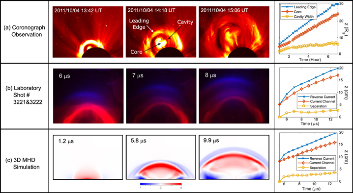
Figure 1. (a) Image sequence of the three-part CME captured by LASCO-C3 on 2011 October 4. This sequence shows a nearly edge-on view of the current channel instead of the perpendicular views shown from the experiment. (b) Image sequence of composite multiwavelength fast camera images of laboratory experiment. Each image consists of two bandwidths: filtered Hα in blue (H-dominated) and visible light in red (Ar-dominated). (c) Cross-sectional plots of simulated current density in the horizontal direction (Jy) showing the propagation of the main current (red) and an induced reverse current layer (blue). For each case, the height evolution of leading edge/reverse current (blue), core/current channel (red), and cavity width/separation (yellow) are plotted in the last column.
Download figure:
Standard image High-resolution imageThe formation of a similar density cavity structure was evident in cylindrical shock tube experiments (Vlases 1963; Hoffman 1967). In these experiments, an increasing axial current induces a reverse current shell, which expands outwards due to the mutual repulsion of the anti-parallel currents, leaving behind a density cavity between the core and reverse currents. This induced reverse current layer is a consequence of the frozen-in condition of MHD: the increasing azimuthal field from the current channel necessarily induces an equal and opposite shell of reverse current to preserve the magnetic flux in the background plasma. This reverse current mechanism was first described in Greifinger & Cole (1961) but has never before been applied to CMEs.
In this Letter, we present measurements of this reverse current mechanism in arched flux-rope experiments and 3D MHD flux-rope simulations that dimensionlessly scale to CMEs. These results show the formation of a density cavity between an increasing core current and a reverse current shell. A simple analytic model for the cavity formation is derived by extending the shock solution from Greifinger & Cole (1961) to a layer of finite width. This model is then shown to be in good agreement with experiment, simulation, and CME observations.
2. Experiment
The experiment generates an expanding flux rope (argon) that collides with a background plasma (hydrogen). The apparatus consists of a magnetized plasma gun mounted at the end of a 1.6 m long, 0.92 m diameter vacuum chamber (Hansen & Bellan 2001; Stenson & Bellan 2012; Ha & Bellan 2016; Wongwaitayakornkul et al. 2017). Figure 2(a) shows the apparatus and Cartesian coordinate system. Two solenoids, one beneath each electrode, are pulsed to produce an arched magnetic field, similar to a horseshoe magnet. This background field ranges from 0.3 T at the footpoints to 0.06 T at the loop apex. Above each solenoid there are gas nozzles connected to fast valves. These valves are pulsed, releasing diverging flows of argon neutral gas in two expanding cones with number density 1019–1022 m−3. A neutral hydrogen prefill, n = 3 × 10²¹ m−3, is added to provide a background gas. Finally, a 59 μF capacitor charged to 3.6 kV is discharged across the electrodes, ionizing the neutral gas and driving up to 30 kA for ∼10 μs through the plasma. Less than 2 kA is carried by the bright collimated loop structure, with the remainder of the current traveling in a broad, diffuse outer envelope. The collimated loop has  , for
, for  m−3, κT = 2 eV, and B = 200 G.
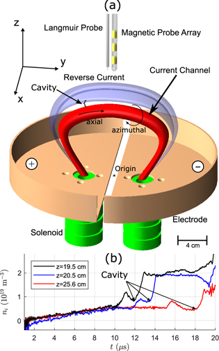
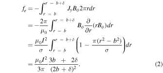
Figure 2. (a) Schematic diagram of the experimental setup showing the primary current channel (red), the induced reverse current layer (blue), electrodes (copper), solenoid (green), magnetic probe array (yellow), and Langmuir probe (gray). (b) Plot of density from Langmuir probe at three locations shows the formation of density cavity.
Download figure:
Standard image High-resolution imageThe dynamics of the current channel and the reverse current are captured by correlating a sequence of visible-light images using a multiple-frame fast camera with measurements made by Langmuir probes and magnetic probes. The false-color images are superimposed with filtered Hα in blue (H-dominated) and visible light in red (Ar-dominated). Using hydrogen gas for the expanding flux rope produced equivalent cavity structures (i.e., ∼2 cm separation) but argon was chosen due to its slower expansion speed and better imaging properties. Figure 1(b) shows the formation and subsequent separation of the reverse current layer from the driving current channel. Langmuir probe measurements shown in Figure 2(b) confirm that the dark cavity region in the experimental images is a region of density depletion (30%–50% lower than the core and reverse current layer). Magnetic measurements from B-dot probes show that the blue feature in Figure 1(b) contains a current oppositely directed to that of the primary injected current channel (red feature). The time dependence of apex positions of the current channel and reverse current layer are tracked from the images and plotted in the far right of Figure 1(b) and are labeled as current channel (i.e., core as in Figure 1(a)) and reverse current (i.e., leading edge as in Figure 1(a)). Because these features have a non-negligible thickness, the locations of the apexes are chosen to be at the center of the feature on the z-axis. The separation (i.e., cavity width as in Figure 1(a)) between the two features is also plotted. The cavity width, defined by the distance between the two apexes, grows quickly and reaches an asymptotic value of 2 ± 0.5 cm. The projected emission in the yz-plane shows that the curvature of the reverse current layer is similar to that of the current channel. The following paragraph describes how the reverse current is calculated from magnetic probe data.
The time dependence of B seen by the probe is from convection rather than diffusion and images show little change in the different features as they move by the probes, i.e.,  . The horizontal current density can therefore be estimated from the time dependence of the magnetic field, i.e.,
  , where
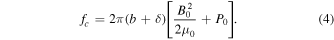
  as measured from feature tracking in fast camera images. Additional magnetic measurements in the xz-plane confirm that the center of the flux rope has spatial variation principally in the z-direction with much less variation in the x-direction (∂xBz ≪ ∂zBx). Figure 3 shows experimental Jy profiles calculated from Bx(t) measurements at three locations (x, y = 0, z = 17.5, 19.5, and 21.5 cm); the inset shows a zoomed-in view of the reverse current, and indicates that this reverse current layer appears spatially ahead of the main current. The spatial distribution and motion of the primary and reverse currents match the features observed in the fast camera images.
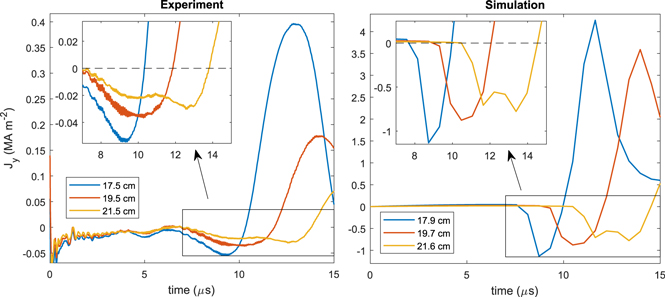
Figure 3. Left panel: calculated Jy(t) profiles at three locations show the distribution and propagation of the reverse current and the current channel in the experiment. The inset shows reverse currents in more detail. Right panel: equivalent plot of Jy obtained from the simulation at three locations analogous to those in the experiment.
Download figure:
Standard image High-resolution imageThe current channel in the experiment expands due to the hoop force, a consequence of greater magnetic pressure on the inboard side of the loop than on the outside (Stenson & Bellan 2012). During this expansion, the current channel collides with the background gas, inducing a reverse current layer of ionized hydrogen.
3. Simulation
To gain further insight into this reverse current layer, the experimental setup was simulated using a 3D MHD equation solver code, a subset of the Los Alamos COMPutational Astrophysics Simulation Suite (LA-COMPASS; Li & Li 2003). This code is described in previous papers simulating the Caltech plasma jet experiment (Zhai et al. 2014) and the arched flux-rope experiment (Wongwaitayakornkul et al. 2017). The ideal MHD code evolves a set of dimensionless parameters: density ρ, pressure P, magnetic field  , and velocity
  on a Cartesian grid with non-reflecting outflow boundary conditions.
The initial density profile consists of (i) exponential cones emerging from the gas nozzles at each footpoint,3
(ii) a uniform background gas  kg m−3, and (iii) a high-density region below z = 0 to simulate the anchoring effect of the electrode boundary. The neutral density in the z > 0 region is
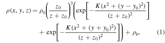
where  kg m−3 is the density at the footpoint,
  , α ≈ 54° is a half cone angle, y0 = 0.04 m is the footpoint location, z0 = 0.01 m is an offset to avoid singularities, and
  kg m−3 is the background density. Initial pressure is defined such that P = (ρ − ρb)κT/mi where mi = mass of hydrogen ion, and κT = 2 eV; the term ρb is subtracted because the background plasma is cold. The plasma is assumed to be initially at rest.
The background magnetic field is constructed from a set of 10 current loops arranged in a half-circle below the footpoints, each with a current of I = 631 kA (see Figure 9 of Wongwaitayakornkul et al. 2017). This arrangement produces a horseshoe-magnet field topology with a magnitude ranging from 0.2 T at the footpoints to 10−3 T at the upper edge of the simulation. The field from each current loop is calculated from a truncated series approximation for the vector potential of an infinitely thin loop (Simpson et al. 2001). This truncation gives an analytic expression for a current loop that is non-singular and divergence-free.
From t = 0 to t = 10 μs, azimuthal flux is added to the domain to match the rising experimental current, Iexp(t) ≈ I0 sin (2πt/T), where T = 40 μs and I0 = 30 kA. This azimuthal magnetic field corresponds to a diffuse arched current constructed from the superposition of 110 current loops and conforms roughly to the shape of the gas cones (i.e., a 54° flared angle at the footpoints). The spatial distribution of the injected current was selected to match the experimental initial conditions, but due to the self-collimating property of parallel currents, the precise spatial profile of the injected current is not critical. The diffuse current is injected via a source term added to the induction equation (Li & Li 2003; Zhai et al. 2014). This incremental addition of flux does not significantly perturb the system at a given time step but slowly increases the poloidal flux, corresponding to a rising current. A more detailed description of this injection scheme can be found in Wongwaitayakornkul et al. (2017).
This setup simulates a flux rope with increasing current that expands into a background plasma. As observed in the experiment, the simulated current channel produces a reverse current layer as the current channel collimates and expands outward. Figure 1(c) plots a time series of Jy from the numerical simulation in the yz-plane, showing a reverse current layer propagating in front of the main current. The shape and position of the main current and reverse current layer are in reasonable agreement with the experiment (±20%), as can be seen by comparing Figures 1(b) and (c). Figure 3 compares the current density Jy in the simulation and in the experiment at the three magnetic probe locations. The experimental current density Jy (left) is broader than in the simulation (right) because of magnetic diffusion from finite resistivity in the experiment. However, the morphology of the profiles are quite similar, as both show a reverse current layer propagating ahead of the core current channel.
4. Snowplow Model for Reverse Current
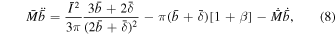
This model extends the infinitely thin snowplow analysis from Greifinger & Cole (1961) to a finite-width reverse current layer and has three key features: an increasing current channel, an expanding reverse current layer, and a density cavity between the current channel and the reverse current layer.
4.1. Assumptions
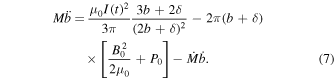
Figure 4 illustrates the model. The configuration consists of a vertical ( ) cylindrical current channel with finite radius a and increasing total current I(t) in a uniform plasma of density ρ0, magnetic field
  , and pressure P0. The current channel is surrounded by a shell/layer of induced reverse current at position b(t), corresponding to the shielding effect of the background plasma. The inner radius of this shell of reverse current is initially at position b(0) = a and the shell is assumed to have a constant thickness δ and a uniform current density Jy = −I/σ across its width, where σ = π(2δb + δ2) is the cross-sectional area of the shell. The motion of the reverse current shell is governed by an expansive force resulting from the mutual repulsion of the oppositely directed currents competing with a restoring force from the background pressure and background magnetic field external to the shell. The cavity region is assumed to have negligible density and pressure (i.e., the "snowplow" assumption). Consequently, there is no outward force on the reverse current from pressure inside the cavity.
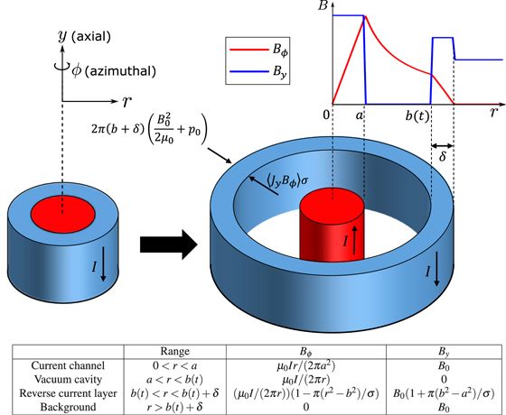
Figure 4. Illustration of the model. The current I is in the +y direction in the main current channel (red) and in the −y direction in the reverse current shell (blue). The reverse current shell has thickness δ and expands radially forming a cavity region between a and b(t). The plot shows the radial dependence of both the normalized axial field (By, blue) and normalized azimuthal field (Bϕ, red). The table lists radial ranges with their corresponding magnetic fields.
Download figure:
Standard image High-resolution imageThe total expansive force-per-length fe is obtained by integrating −JyBϕ over the reverse current layer:
Taking the limit  recovers the expression from Greifinger & Cole (1961), i.e.,

The total confining force fc is calculated as the product of the background pressure and the shell outer perimeter:
This gives the equation of motion for the expansion of the current layer to be

Using the snowplow assumption, the mass-per-length M scales with the swept area, so

The full equation of motion for the current layer can therefore be written as
The last term on the right-hand side is a consequence of momentum conservation from the increasing mass of the layer. A complete void with By = 0 and zero plasma pressure is not observed in the experiment. However, even without many of the features present in the continuous 3D system, the analytic model can characterize the bulk forces and predict cavity widths and internal currents for the experiment and simulation.
4.2. Non-dimensional Form and Equilibrium
Equation (7) can be put in dimensionless form to compare plasmas having different scales. The characteristic velocity is chosen to be the Alfvén speed  and the characteristic time is chosen to be the Alfvén crossing time τ = a/vA. This choice of normalization has three free parameters, B0, a, and ρ0, so Equation (7) becomes
where normalized values are indicated with a bar, (i.e.,  ,
,  ) and
) and  . In both the experiment and the simulation, the cavity width prescribed by Equation (8) reaches equilibrium within a few Alfvén crossing times (i.e., t ∼ 5a/vA). This fast equilibration time implies that cavity widths are relatively independent of the current injection timescale. Solving for this equilibrium (
 ,
,  ) gives
For δ ≪ beq, the solution is a simple pressure balance where  . In dimensioned quantities, the equilibrium cavity size is
  , where I is the main current and B0 is the background field. Since the dependence on plasma β is weak, and the mechanism is independent of the collisional mean free path, the effects should be similar across a wide range of plasma parameters.
4.3. Core Acceleration
The effects of an accelerating frame can be quantified by substituting [b(t)−h(t)] for b(t) in the expansive term, where h(t) represents the height of the loop apex as a function of time, so Equation (2) becomes
This substitution effectively shifts the central current channel (the red cylinder in Figure 4) off-axis with speed ∂th(t). However, for speeds ∂th(t) ≪ vA, the cavity width is not significantly affected and the cavity again reaches an equilibrium width within a few Alfvén crossing times. Equivalently, the system reaches a similar equilibrium width in a moving frame if the momentum conservation term  is small compared to the magnetic terms. This limit is a reasonable approximation for the cases of interest, and the next section will show that the cavity widths predicted by the stationary model agree well with the experiment, simulation, and CME observations. Consequently, the model can be used to infer the internal current
  from cavity width for both stationary flux ropes and flux ropes moving at sub-Alfvénic speeds.
5. Scaling to CMEs
The understanding gained from the experiment, simulation, and theory provide new insights for interpreting the three-part structure of CMEs. The leading edge, cavity, and core elements of a CME respectively correspond to the reverse current layer, the cavity, and the central current channel of the model. This new interpretation is a flux-rope model that identifies where currents are flowing: the main current channel is the core, the cavity is a region of expanding azimuthal flux around the main current channel, and the leading edge corresponds to a compressed reverse current layer between the core current and background plasma.
It is important to evaluate how the experiment and simulation scale to the solar situation. To do this, we follow the MHD scaling method in Ryutov et al. (2000) and so normalize each system using the current channel minor radius a as a reference length, a reference magnetic field B0, and a reference density ρ0. The reference time for normalization is then given by  . The reference parameters for both the simulation and experiment are a = 5.0 × 10⁻³ m, B0 = 0.01 T,
  ,
,  . The reference parameters for the 2011 October 4 CME event are a = 1.0 × 10⁹ m,
  T (Bastian et al. 2001; Maia et al. 2007),
  kg m−3, and τ0 = 710 s. The density is estimated from a typical CME mass M = 1012 kg (Vourlidas et al. 2010) divided by the core volume, πa2πR, using major radius R = 5a. The laboratory, simulation, and CME event can then all be expressed in terms of the same dimensionless variables.
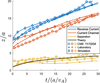
Figure 5 compares the scaled height and time of the leading edge and core, as well as the separation between the leading edge and core, for theory, simulation, experiment, and CME observations. Separation is defined as the center-to-center distance between the main current channel and the reverse current shell. The center of the reverse current shell is at  . The theoretical black line is calculated by solving Equation (8) with
  ,
,  ,
,  , and a sinusoidal ramping current,
 ![$\bar{I}=[{\bar{I}}_{0}+20\sin (\pi \bar{t}/60)]$](https://content.cld.iop.org/journals/2041-8205/862/2/L15/revision1/apjlaad33cieqn34.gif) where
where  is set such that the system is initially at equilibrium. This dimensionless current corresponds to an experimental current of 1 kA and a solar current of ∼5 × 10¹² A. This agreement of normalized parameters in Figure 5 indicates that the reverse current mechanism can reproduce the observed three-part structure at the solar scale.
Figure 5. Comparison of the cavity width for all the different scenarios, taken from the right column of Figure 1. Color: (blue) reverse current, (red) current channel, (yellow) separation, and (black) theory ( ). Style: (o) CME on 2011 October 4, (x) laboratory, and (
 ) simulation. In this plot, the separation is defined as the center-to-center distance between the main current and the reverse current layer. Vertical error bars are ±0.5 for all traces. The black line represents a numerical solution to Equation (8) with
  and
and ![$\bar{I}=[{\bar{I}}_{0}+20\sin (\pi \bar{t}/60)]$](https://content.cld.iop.org/journals/2041-8205/862/2/L15/revision1/apjlaad33cieqn39.gif) .
.
Download figure:
Standard image High-resolution image
This work was supported by NSF under award 1348393, AFOSR under award FA9550-11-1-0184, and DOE under awards DE-FG02-04ER54755 and DE-SC0010471. H.L. acknowledges support from the DoE/OFES and LANL/LDRD programs.
Footnotes
- 3
Without background gas, the cone density decays as z−2 (Yun 2008). The presence of background gas impedes the expansion of gas exiting from the nozzles so the gas cone density decays more rapidly with increasing z; this more rapidly decaying density was modeled as having a profile scaling as z−3.