


Abstract
Supernova explosions are among the most energetic events in the Universe. After the explosion, the material ejected by the supernova expands throughout the interstellar medium (ISM), forming what is called a supernova remnant (SNR). The shocks associated with the expanding SNR are sources of galactic cosmic rays, which can reach energies of the PeV order. The magnetic field plays a key role in these processes. It is known that the ISM is turbulent, with an observed magnetic field of about a few μG, made by the superposition of a uniform and a fluctuating component. During the SNR expansion, the shock interacts with this turbulent environment, leading to a distortion of the shock front and a compression of the medium. In this work, we use the magnetohydrodynamics PLUTO code to mimic the evolution of the blast wave associated with an SNR. We perform a parametric study varying the level of density and magnetic field fluctuations in the ISM, with the aim of understanding the best parameter values able to reproduce real observations. We introduce a novel analysis technique based on a two-dimensional autocorrelation function C(ℓ) and a second-order structure function S2(ℓ), quantifying the level of anisotropy and the turbulence correlation lengths. By interpolating the autocorrelation function on a polar grid, we extract the power spectra of turbulence at the SNR. Finally, a preliminary comparison with Chandra observations of SN 1006 is also presented.

Original content from this work may be used under the terms of the Creative Commons Attribution 4.0 licence. Any further distribution of this work must maintain attribution to the author(s) and the title of the work, journal citation and DOI.
1. Introduction
A supernova (SN) explosion is an instantaneous release of energy of about ≃1051 erg, associated with the catastrophic collapse of a massive star or due to the runaway nuclear burning of a white dwarf. After a SN explosion, the material ejected from its progenitor permeates the interstellar medium (ISM), expanding at a speed that can exceed the local sound speed. This gives rise to a shock front, also known as a forward shock (FS), which tends to be slowed down by its interaction with the ISM. Thus, the FS undergoes deceleration as it sweeps up material. The ejecta tends to catch the shock and a reverse shock (RS) is generated, propagating backward in the reference frame of the ejecta. Between these two shocks an interface region forms, called the contact discontinuity (CD). This is a boundary region between the part of the ejecta heated by the RS and the other part heated by the FS–ISM interaction. The expanding material collected by the blast wave during its evolution through the ISM gives rise to a supernova remnant (SNR). Three phases can be recognized in the evolution of an SNR: (1) the free-expansion phase, characterized by a FS moving at almost constant speed into the ISM (in this phase the amount of material swept up by the shock is smaller than the mass of the ejecta); (2) the Sedov–Taylor phase (or energy-conserving phase), when the mass of the swept-up gas exceeds the mass of the ejecta and the kinetic energy of the explosion is transferred to the swept-up material, which does not radiate; and (3) the radiative phase dominated by radiation losses, involving several emission lines, during which the shock slows down and the gas becomes cooler (J. C. Raymond 1979; E. A. Helder et al. 2012).
It is widely believed that SNR shocks are the sources of Galactic cosmic rays, whose energy can reach 1015 eV, and also sources of X-ray and radio emissions. These high-Mach-number shocks can accelerate energetic particles at relativistic energies through the diffusive shock acceleration mechanism, in which particles can cross the shock back and forth due to the scattering with magnetic irregularities, gaining an amount of energy at each crossing (E. Fermi 1949; G. F. Krymskii 1977; A. Bell 1978a; A. R. Bell 1978b; R. D. Blandford & J. P. Ostriker 1978; J. Jokipii 1982, 1987; L. O. Drury 1983; F. Guo et al. 2010; S. Liu & J. R. Jokipii 2021). In these high-energy processes, a key role is played by the magnetic field. It is known that the ISM is turbulent, with a Kolmogorov-like power spectrum (L. C. Lee & J. R. Jokipii 1976; J. W. Armstrong et al. 1981, 1995; A. Chepurnov & A. Lazarian 2010; J. L. Linsky et al. 2022b; J. Linsky et al. 2022a). Observations have revealed that the Galactic magnetic field assumes values of a few μG, and is given by the superposition of a uniform and a random/fluctuating component which are approximately in equipartition (R. Beck et al. 1996; A. H. Minter & S. R. Spangler 1996; J. L. Han et al. 2004). Turbulence is one of the most important physical processes in astrophysics, spanning from cosmology to the ISM, including stars, SN explosions, accretion disks, and much else (D. Radice et al. 2018; C. Meringolo et al. 2023; C. Wang et al. 2024). It is ubiquitous in the Universe, and the dynamics of nonstationary astrophysical plasma include a wide range of length scales, velocities, and timescales. Hence, the study of this phenomenon can help to understand its key role in the generation of large-scale magnetic fields that characterize many celestial objects. The ISM turbulence scales range from kiloparsecs to several astronomical units (J. W. Armstrong et al. 1995; B. G. Elmegreen & J. Scalo 2004; A. Brandenburg & A. Lazarian 2013). Magnetohydrodynamic turbulence therefore plays a fundamental role in astrophysical processes in the ISM. The role of MHD turbulence has been tested in recent decades with the support of numerical simulations, which have confirmed many theoretical predictions (A. Kolmogorov 1941; J. V. Shebalin et al. 1983; J. Cho & A. Lazarian 2005; A. G. Kritsuk et al. 2007; C. Federrath et al. 2010; C. Federrath 2016; R. Ferrand et al. 2019).
Several studies have investigated the interaction between turbulent magnetic fields and shock waves. Such an interaction can distort the shock surface, leading to the formation of shock ripples (L. Ofman & M. Gedalin 2013; A. Johlander et al. 2016), and to an increase of the fluctuation level in the downstream region (M. Neugebauer & J. Giacalone 2005; Q. Lu et al. 2009; D. Trotta et al. 2021; M. Nakanotani et al. 2022). The process of magnetic field amplification due to the turbulent dynamo has widely been explored, making use of MHD simulations with one-dimensional (J. R. Dickel et al. 1989), two-dimensional (J. Giacalone & J. R. Jokipii 2007; T. Inoue et al. 2009; F. Guo et al. 2012; F. Fraschetti 2013; Y. Mizuno et al. 2014), and three-dimensional (T. Inoue et al. 2013; S. Ji et al. 2016; Y. Hu et al. 2022) configurations. These works show that turbulence can amplify the magnetic field in the postshock region by a factor of 100.
The interaction between shocks associated with SNRs and the turbulent ISM has been intensively studied in F. Guo et al. (2012), H. Yu et al. (2015), and P. F. Velázquez et al. (2017). In particular, F. Guo et al. (2012) developed a two-dimensional MHD simulation in which they studied the amplification of the magnetic field when a SN blast wave propagates into a turbulent ISM. Two different processes can affect the magnetic field amplification: (1) the interaction between the shock front and the turbulent environment that allows the formation of the shock ripples, which amplify the magnetic field; (2) the growth of the Rayleigh–Taylor instability (RTI) at the CD region, which produces the highest amplification of the magnetic field. RTI occurs when two fluids of different densities interact. When an impulsively accelerated shock wave propagates between two fluids with different densities, an evolution of the RTI appears, called the Richtmyer–Meshkov instability (RMI; R. D. Richtmyer 1960; E. E. Meshkov 1969). The RMI is believed to be responsible for the amplification of the magnetic field in SNRs (T. Sano et al. 2012; S. R. Nagel et al. 2017). A secondary instability, namely the Kelvin–Helmholtz instability (KHI), can also induce turbulence. It develops when a shear of velocity appears at the interface between two fluids (Helmholtz 1868; W. Thomson 1871). The KHI plays an important role in various regions of the solar system, such as planetary magnetopauses, the solar atmosphere, and solar wind; but also in astrophysical systems such as pulsar wind nebulae and around quasars (A. Masson & K. Nykyri 2018).
Y. Hu et al. (2022) compared two-dimensional and three-dimensional MHD simulations of shock propagation inside a dense turbulent environment. They found differences in terms of morphology and amplification of the magnetic field. Three-dimensional simulations show larger amplification than two-dimensional simulations and, as a consequence, the morphology of the shock looks quite different, with a more corrugated shock front and the development of filaments.
To better understand the influence of turbulence on the transport properties of the blast wave in an SNR, it is fundamental to explore all the possible configurations of the ISM background, performing a parametric study of the shock–turbulence interaction, in order to "tune" the simulation parameters for comparison with observations.
Particle acceleration in SNR shocks is evidenced by the presence of synchrotron emission from relativistic electrons. The emission is brighter at the edges of the blast waves, giving rise to bright rims (G. Morlino et al. 2010) where particle acceleration processes occur. The magnetic field can also be amplified by the presence of energetic particles streaming back ahead of the shock (E. Amato 2014) exciting low-frequency waves that locally enhance the magnetic field (A. Bell 2004). Actually, the presence of turbulence in the upstream region can be the cause of the irregular emissions seen in SNRs and also of the particular shape that the edges of the shock assume when they interact with the ISM (M. C. Anderson & L. Rudnick 1996; D. Balsara et al. 2001; F. Guo et al. 2012; E. M. Reynoso et al. 2013; H. Yu et al. 2015). Such an irregular and nonuniform emission has been observed in SN 1006, a Type Ia SN, i.e., the result of the explosion of a white dwarf in an accretion binary system. In these systems white dwarfs increase their mass from a companion that can be any type of star. The companion pushes the white dwarf over the Chandrasekhar limit into core collapse, resulting in a total disruption of the star. There is no stellar remnant in this case, such as a neutron star or black hole (K. W. Weiler & R. A. Sramek 1988). SN 1006 has a bilateral morphology consisting of two bright limbs located in the northeastern part (NE) and in the southwestern part (SW), that present knots and filaments along the boundary of the remnant (K. Koyama et al. 1995; A. Bamba et al. 2003; R. Rothenflug et al. 2004; E. M. Reynoso et al. 2013). The NE and the SW regions mainly emit in the radio and X-ray bands, which correspond to the synchrotron emission from high-energy electrons, while the gamma-ray band could be associated with high-energy protons. Synchrotron emission is responsible for both the nonthermal emission in the radio band and the X-ray band.
This paper aims to mimic the interaction between a shock associated with the expansion of an SNR within a turbulent ISM. Since the properties of the turbulence in the ISM around an SNR shock are difficult to infer, we make use of numerical simulations in modeling the turbulent conditions of the ISM to better reproduce observations. In particular, we focus on SN 1006, which is an old SNR largely studied in the literature (A. Bamba et al. 2003; G. Cassam-Chenai et al. 2008; M. Miceli et al. 2009; S. Orlando et al. 2012, 2021; S. Perri et al. 2016). By systematically varying the properties of the turbulence, we aim to understand how the turbulent ISM influences the expansion of SN 1006.
The evolution of SN 1006 is reproduced by using the MHD PLUTO code (A. Mignone et al. 2007, 2011), setting different turbulent conditions in the ISM, both in the density and in the magnetic fields.
We perform a parametric study which allows us to determine the factors that mostly affect the SNR expansion. Finally, we implement an analysis of the turbulence anisotropy within the remnant, after its interaction with the ISM, by means of a novel technique to estimate the power spectra. This is based on the study of the two-dimensional autocorrelation function. We apply a ring-shaped mask to the SNR, from which we extract the two-dimensional autocorrelation function and the structure function. We then interpolate both into polar coordinates in order to measure the correlation length at fixed angle values. For each angle, we compute the power spectra by applying the Blackman–Tukey technique (R. B. Blackman & J. W. Tukey 1958a, 1958b).
Such a procedure will also be applied to Chandra observations of SN 1006 in the 1–3 keV energy band for qualitative comparison with numerical simulations.
2. Numerical Model
To reproduce the dynamical evolution of an SNR blast wave propagating through a magnetized environment, we use the time-dependent, ideal, MHD equations of mass, momentum, and energy conservation in a Cartesian coordinate system. We choose to integrate these equations by using the PLUTO code (A. Mignone et al. 2007, 2011). PLUTO is a Godunov-type code that provides a modular computational framework for the solution of gas dynamics equations under different regimes.
The governing MHD equations used in the code are as follows:

Equations (1) are dimensionless, and are normalized to a typical length (L0 = 1 pc), velocity (v0 = 105 cm s−1), and density (ρ0 = 1.6724 gr cm−3), as is usually done in the PLUTO code (A. Mignone et al. 2007). Here, ρ = μntotmp is the mass density, where μ is the mean molecular weight, ntot the total number density of the particle and mp the proton mass, v = (vx, vy, vz) the fluid velocity, B = (Bx, By, Bz) the magnetic field, and Pt the total gas pressure, i.e., the sum of the thermal and the magnetic pressure (Pt = P + B2/2). At this stage, we do not take into account the effects related to thermal conduction, viscosity and resistivity, radiative cooling, and nonlinear effects due to the acceleration of charged particles. We couple this set of equations with an equation of state for an ideal gas. The total energy density is , where γ is the adiabatic index. The solutions of the MHD equations must satisfy the divergence-free condition, i.e., ∇ · B = 0. This condition is not naturally preserved in numerical schemes without a proper technique. PLUTO uses three different techniques in order to fulfill the condition ∇ · B = 0: the eight-wave formulation (K. Powell 1994; K. G. Powell et al. 1999), hyperbolic divergence cleaning (A. Mignone & P. Tzeferacos 2010; A. Mignone et al. 2010), and constrained transport (CT; D. S. Balsara & D. S. Spicer 1999; P. Londrillo & L. Del Zanna 2004). In the eight-wave formalism the magnetic field has a cell-centered representation and additional terms (source terms) are added to the ideal MHD equations and, depending on the Riemann solver used, the source terms can be discretized in different ways. In hyperbolic divergence cleaning the divergence-free condition is enforced by solving a modified system of conservation laws, in which the induction equation is coupled with a generalized Lagrange multiplier. This technique is useful because no source terms are introduced, so the equations retain a conservative form, all variables retain a cell-centered representation, and it is possible to use different Riemann solvers. The CT formalism uses two sets of magnetic fields: a face-centered field and a cell-centered field. In the first one the field components are located at different spatial points in the control volume, while in the second one the staggered magnetic field is treated as an area-weighted average on the zone face and Stokes' theorem is used to update it. In this work we advance the magnetic field and, to preserve the divergence-free condition, we use the CT formalism, though the results are consistent when using the other two schemes.

2.1. Numerical Setup
We set up simulations in two-dimensional Cartesian coordinates (x, y) with uniform grids. The computational domain extends from −30 to 30 pc in both directions sampled with a total of 40962 grid points. We set all the other quantities following S. Orlando et al. (2012) and F. Guo et al. (2012). In particular, we assume an initial cylindrical remnant of radius RSN,0 = 0.4 pc and length in the z-direction of Lz = 0.8 pc that corresponds to an age of t0 = 10 yr, whose progenitor is a star with a mass of 1.4 M⊙. We set the internal energy within the cylinder area equal to Einj = 1.5 × 1051 erg. This allows us to define an internal initial number density of about ninj = 13.3 cm−3. The environment in which our remnant is evolving is set with a uniform density n = 0.1 cm−3 (G. Morlino et al. 2010; S. Perri et al. 2016) and a uniform temperature T = 104 K. The shock associated with the SNR is supposed to expand with a velocity Vsh ≃ 4400 km s−1 and the adiabatic index is chosen as γ = 5/3 for a monoatomic, nonrelativistic, ideal gas. We follow the SNR expansion until 10 pc; at this stage, the SN is in the Sedov–Taylor phase and the energy is conserved because we do not take into account radiative losses. We set a background mean magnetic field B0 = 3 μG, and we can vary its direction to span different case studies. The direction of the mean magnetic field in spherical coordinates is given by

In order to make a comparison with SN 1006, we choose ϕ = 150∘ and , where ϕ is the azimuthal angle and the colatitude. These values are deduced from observations in E. M. Reynoso et al. (2013), where the mean magnetic field has been found to be oriented at 60∘ with respect to the Galactic plane normal.


2.2. Homogeneous Turbulence
A compressible turbulent background in which the SNR blast wave propagates has been set as an initial condition of our simulations. Indeed, we consider the ISM as being made of density and magnetic field fluctuations superposed to a background field. We initialize the in-plane magnetic field as done in classical simulations of plasma turbulence (S. Servidio et al. 2012; C. Meringolo et al. 2024). Since we want to reproduce realistic conditions for the interstellar background medium, we consider different spectra for both fields. We start by expressing the z-component of the vector potential in Fourier modes as

where k = (kx, ky) is the k-vector, k = ∣k∣, and are random phases. In the above equation, sets the initial shape of the spectrum, peaking at k = k0 = (2π/L)m0 with m0 = 4, L = 60 pc, and with a power law α = 15/6. The magnetic field is therefore computed as B = ∇ × A, so that, according to Equation (2), its power spectral density follows a Kolmogorov-like decay with P(k) ∼ k−5/3, as observed at intermediate scales in astrophysical plasma turbulence (R. Bruno & V. Carbone 2013). Such an initial condition consists of random fluctuations on a wide range of scales. We set a smooth cutoff in the Fourier space at k* = 50 to ensure that we can avoid possible aliasing effects at any used resolution (C. Meringolo et al. 2021). Figure 1(a) shows the initial power spectrum of the total magnetic field. Note that the Kolmogorov spectrum is also plotted for comparison. In Figure 1(b), we report the contours of the initial magnetic field, obtained from the Az potential vector, in the (x, y) plane.

![$\widetilde{A}(k)={[1+{(k/{k}_{0})}^{\alpha }]}^{-1}$](https://content.cld.iop.org/journals/0067-0049/277/2/44/revision2/apjsadb62fieqn5.gif)

Figure 1. (a) Power spectral density of the total magnetic field (blue solid line). The dashed–dotted line represents the Kolmogorov scaling. (b) Initial magnetic field obtained by computing the curl of the Az potential vector.
Download figure:
Standard image High-resolution imageSince we know that in stellar wind, and in particular in the solar wind, density fluctuations can assume a log-normal probability distribution (L. Burlaga et al. 2006), we set the density field as following a log-normal distribution (J. Giacalone & J. R. Jokipii 2007):

where f0 is a properly chosen constant, and δf is the density perturbation. We build the spectrum of δf in a way analogous to the one we used for the vector potential in Equation (2). Before applying the exponential function to the density fluctuations, we normalize the argument to unity in order to avoid extreme values. The spectrum of density fluctuations is plotted in Figure 2(a). The initial density field is also reported in Figure 2(b).

Figure 2. (a) Power spectrum of the density (green solid line). (b) Background density map.
Download figure:
Standard image High-resolution image3. Simulation Results
All the runs performed are summarized in Table 1. In particular, we chose Run 2 (in bold in Table 1) as a reference simulation. In Run 2 the level of magnetic field turbulence is set to δB/B = 0.5 (F. Guo et al. 2012), while the level of density fluctuations is δn/n = 1. We fix the number density of the background close to the typical value of the ISM (G. Morlino et al. 2010; S. Perri et al. 2016).
Table 1. List of the Numerical Runs Performed
| Run | Mej | nout | δB/B | δn/n | Bavg | navg | ||
|---|---|---|---|---|---|---|---|---|
| (M⊙) | (cm− 3) | (μG) | (μG) | (cm−3) | (cm−3) | |||
| 1 | 1.4 | 0.1 | 0.1 | 1 | 4.88 | 425.1 | 0.42 | 2.29 |
| 2 | 1.4 | 0.1 | 0.5 | 1 | 5.1 | 475.5 | 0.42 | 2.29 |
| 3 | 1.4 | 0.1 | 1 | 1.0 | 5.8 | 521.6 | 0.42 | 2.29 |
| 4 | 1.4 | 0.1 | 0.5 | 0.1 | 6.2 | 609.5 | 0.15 | 0.7 |
| 5 | 1.4 | 0.1 | 0.5 | 0.5 | 5.5 | 474.2 | 0.27 | 1.43 |
| 6 | 3 | 0.1 | 0.5 | 1 | 4.3 | 480.6 | 0.46 | 3.8 |
| 7 | 5 | 0.1 | 0.5 | 1 | 3.82 | 415.9 | 0.5 | 6.99 |
| 8 | 1.4 | 0.05 | 0.5 | 1 | 5.95 | 563.3 | 0.22 | 1.57 |
| 9 | 1.4 | 1 | 0.5 | 1 | 3.4 | 74.7 | 4.03 | 18.26 |
| 10 | 1.4 | 3 | 0.5 | 1 | 3.24 | 18.3 | 11.8 | 54.6 |


Note. The values of the mass of the ejecta, the magnetic and the density turbulence level, the mean and the maximum magnetic field values, the mean and the maximum density values, calculated over the whole simulation box at the final time in each simulation, are reported.
Download table as: ASCIITypeset image
In Figure 3, we show for Run 2 at the final simulation time, t = 3 × 10³ yr, the spatial distributions of the number density, the kinetic pressure, the gas temperature, the velocity components, and the magnetic field intensity. At the beginning of the simulation, the ejecta is characterized by high values of density and pressure, such that a strong shock in the turbulent background is induced, heating and compressing the ambient medium. Since the shocked circumstellar medium pushes back the ejecta, a RS is produced. In Figure 3, the RS extends up to about 10 pc, while the FS expands beyond 20 pc.

Figure 3. Spatial distribution of (a) number density, (b) pressure, (c) temperature, (d) and (e) x- and y-components of the velocity, and (f) the magnetic field magnitude from Run 2 at an age of 3000 yr.
Download figure:
Standard image High-resolution imageBetween the FS and RS, the CD emerges, where the RTI is triggered (D. H. Sharp 1984). Outside the inner ejecta, the region known as the outer ejecta extends up to the FS, characterized by very high values of compression. The interaction between the expanding FS and the dense ISM distorts the shock surface. To better characterize the FS, its magnetic compression ratio rB = Bdown/Bup, where Bdown is the downstream magnetic field and Bup is the upstream magnetic field, is calculated in the region in which the shock is quasi-perpendicular. We find that rB = 2.5 is comparable with the ratio between the downstream (ndown) and the upstream (nup) densities, namely ndown/nup = 2.4, which is what is expected at perpendicular shocks. Figures 3(b) and (c) show the pressure and temperature maps. The pressure map shows a behavior similar to the density, with higher values in the FS region. The temperature map shows higher values in the region where the RTI dominates. Finally, the magnetic field exhibits a noticeable amplification and compression in the direction perpendicular to the direction of the mean magnetic field. The background magnetic field fluctuations tend to distort the shape of the FS and, as a result, it is possible to observe knots and filaments in this region, which are reflected also in the inhomogeneous profiles of the kinetic pressure and temperature. More details can be observed in Figure 4, where zoom ins of the spatial distributions of the number density and magnetic field amplitude are presented. It is possible to see the structures formed by the triggered RTI and the deformation of the FS due to the interaction of the ejecta with the turbulent environment. The density map shows a more uniform compression in the FS region, while the magnetic field map shows a higher level of distortion in the shock surface and magnetic field amplification in the regions where B is tangential, according to the Rankine–Hugoniot conditions. Notice that E. M. Reynoso et al. (2013) present a radio polarization study of SN 1006, finding that particles are efficiently accelerated along the direction of the mean magnetic field (namely in the NE and SW shells of the remnant). On the other hand, we perform purely MHD simulations. In our case, the magnetic field is amplified in the northwestern part and the southeastern part, in agreement with the Rankine–Hugoniot jump conditions for an ideal MHD shock; indeed, in such regions the mean magnetic field is almost perpendicular to the shock normal, thus resulting in a higher B compression. In our simulations, we neglect the contribution of the particle acceleration that plays a key role in magnetic field amplification (A. Bell 2004), a mechanism that will be explored in future works. Nevertheless, wherever emission is high our analysis technique can shed light on the turbulent properties of the medium.

Figure 4. Zoom ins of the spatial distributions of (a) the number density and (b) the magnetic field amplitude.
Download figure:
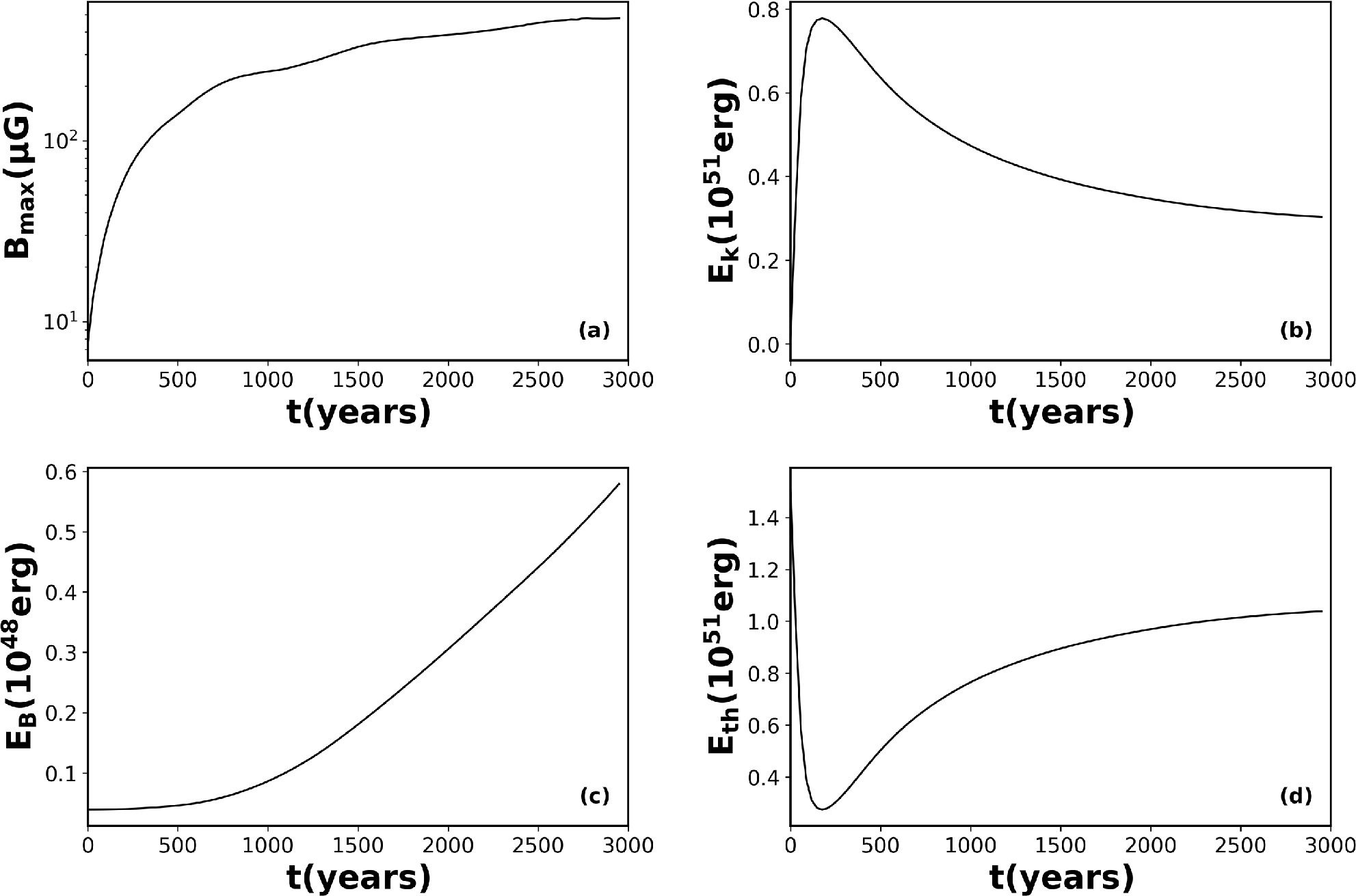
Standard image High-resolution imageIn order to give an idea of the SNR evolution, we trace in Figure 5 the time evolution of the maximum magnetic field attainable in the simulation, and the time behavior of the kinetic, magnetic, and thermal energies. The energies are averaged over the whole simulation domain.

Figure 5. (a) Time evolution of the maximum value of the magnetic field in the domain, (b) the total kinetic energy, (c) the magnetic energy, and (d) the thermal energy, all averaged over the whole simulation domain.
Download figure:
Standard image High-resolution imageThe maximum value of ∣B∣ shows a linear increase until ≃600 yr, at which time it reaches 250 μG. After a brief period during which a little plateau appears (around 500 yr), it rapidly increases until 3000 yr, reaching a maximum value of 475 μG. The values obtained for the maximum amplification of the magnetic field strength are determined over the whole simulation box for each run (see Table 1). We then calculate the mean magnetic field strength within the region between the RS and the FS. We find at 3 × 10³ yr Bmean ≃ 13 μG and a maximum value of 475 μG; that is, the magnetic field amplification can reach up to almost 2 orders of magnitude with respect to the value of 3 μG in the ISM. This result is in agreement with observations of SN 1006 reported by S. M. Ressler et al. (2014), in which the magnetic field value is of the order of 100 μG.

The behavior of the maximum value of the magnetic field is reflected in the magnetic energy, which continuously increases, reaching a maximum value of ∼0.6 × 1048 erg. These results are in agreement with the ones found by J. Giacalone & J. R. Jokipii (2007) and F. Guo et al. (2012). Figures 5(b) and (d) show that the kinetic energy increases rapidly until 200 yr due to the high density and pressure that drive the strong shock in the turbulent ISM, while the thermal energy decreases rapidly with the same behavior. During this rapid increase, the kinetic energy reaches a maximum value of ∼0.8 × 1051 erg, which corresponds to a conversion of about 54% of the thermal energy. After that, the ejecta slows down due to interaction with the turbulent ISM, so that the kinetic energy slowly decreases and the thermal energy increases. This happens because the total energy is mostly conserved and the magnetic energy remains much smaller than the other two.
In Figure 6, we show the time evolution of (a) the SNR radius and (b) the FS speed. Since the ejecta is expanding in a dense and turbulent environment, the shock velocity constantly decreases. The shock speed decreases from about 6000 to 3000 km s−1, in agreement with the theoretical evolution of the FS speed in the Sedov–Taylor phase, i.e., Vsh ∝ t−3/5 (E. A. Helder et al. 2012). The radius of the FS also increases and approaches the power-law behavior predicted in the Sedov–Taylor phase r ∝ t2/5 (R. A. Chevalier 1982; F. Guo et al. 2012; E. A. Helder et al. 2012).

Figure 6. Time evolution of (a) the FS radius and (b) the FS speed in Run 2. A comparison with the trends predicted by the Sedov–Taylor phase is also given (red dashed lines).
Download figure:
Standard image High-resolution image3.1. Statistical Analysis of Turbulence at SNRs
We investigate the level of turbulence anisotropy related to the presence of a strong background magnetic field. J. V. Shebalin et al. (1983) found that, starting from an initially isotropic spectrum, anisotropy develops also with a modest amplitude of the mean magnetic field. Different levels of anisotropy can also be found in different regions of the solar wind (S. Dasso et al. 2005; J. M. Weygand et al. 2009; F. Sahraoui et al. 2010; C. Chen et al. 2011; R. Bandyopadhyay & D. J. McComas 2021; F. Pecora et al. 2023). To study the properties of the turbulence, we use a novel technique in which we apply a Heaviside mask (ring-shaped) to the density and magnetic field maps, to select the region between the RS and the FS only. Thus, we calculate the two-dimensional structure function S2(ℓ) of the magnetic field turbulence inside that ring-shaped mask as

where δB(r) = B(r) − B0, ℓ represents a spatial lag, and r is the position in the simulation domain. Once we determine the structure function, we can calculate the autocorrelation function as Cb(ℓ) = (Cb(0) − S2(ℓ)/2)/Cb(0). In order to explore the deep statistical properties of the turbulence, we also calculate the correlation length λc. The correlation length is defined as the e-folding distance of the normalized autocorrelation function (C. W. Smith et al. 2001). It gives us a measure of the size of the turbulence structures. The same approach has been adopted for the density field. In Figures 7 and 8, the outputs of the above analysis are displayed for the density map and magnetic field map, respectively.

Figure 7. (a) Density map distribution after the application of the ring-shaped mask (overplotted in gray), located within the CD. (b) Autocorrelation function map computed on the ring-shaped region. The red solid line represents the autocorrelation length, namely the isocontour of C2 = 1/e. ℓx and ℓy are the increments along the x- and y-directions, respectively.
Download figure:
Standard image High-resolution image
Figure 8. Same as Figure 7 but for the magnetic field spatial map.
Download figure:
Standard image High-resolution imageFrom Figure 7, the autocorrelation density map appears to be anisotropic, elongated along the direction perpendicular to the mean magnetic field. A similar result has been observed for the magnetic field map, where the largest values of the correlation length are detected perpendicular to the mean magnetic field .
In addition, the density field tends to be more correlated over larger spatial scales. In both cases the explanation comes from the structures emerging in the CD due to the RTI.
3.1.1. Simulations with Different Background Turbulence Levels
We now discuss how variation of the simulation parameters reported in Table 1 affects the evolution of the SNR.
Figure 9 compares the spatial maps of the density and magnetic fields in Runs 1–3, where the level of magnetic field turbulence varies and the density fluctuations are fixed. The density field does not exhibit a significant variation with the δB/B parameter, while the magnetic field in the SNR reacts to the amplitude of the ISM perturbed field in terms of the formation of knots and filaments. Furthermore, as expected, an increase of the magnetic field turbulence leads to an enhancement of the magnetic field magnitude along the shock. In Figure 10, results from Runs 2, 4, and 5 are presented. Unlike the previous case, as the δn/n increases, the density maps show a stronger deformation of the shock surface. As a consequence, the SNR radius decreases. In the case of the magnetic field maps (Figures 10(d)–(f)), we do not observe variation in terms of magnetic field amplification, and the only difference is again related to the radius of the remnant. We can conclude that when we set δn/n to a small value, even if we vary δB/B, the rest expands in the same way in the three cases. Instead, when we fix δB/B and vary δn/n, the expansion is slowed down.

Figure 9. Spatial distribution of (a)–(c) the number density and (d)–(f) the magnetic field magnitude from the two-dimensional simulation at an age of 3000 yr in Run 1, Run 2, and Run 3.
Download figure:
Standard image High-resolution image
Figure 10. Spatial distribution of (a)–(c) the number density and (d)–(f) the magnetic field magnitude from the two-dimensional simulation at an age of 3000 yr in Run 4, Run 5, and Run 2.
Download figure:
Standard image High-resolution imageIn Figure 11, the averaged energies and the maximum magnetic field time behavior over the three simulations are displayed. For comparison, the red line in each panel represents a simulation with a uniform and nonturbulent ISM. The magnetic energy and the maximum value of ∣B∣ reach higher values as the amplitude of the magnetic field fluctuations increases (Figures 11(a) and (c)).

Figure 11. Same quantities as in Figure 5. The blue, green, and purple lines indicate Run 1, Run 2, and Run 3, respectively. The red line represents the nonturbulent case.
Download figure:
Standard image High-resolution imageThe values observed in Figure 11 are in agreement with the results obtained by F. Guo et al. (2012) and S. Xu & A. Lazarian (2017). In particular, the values of in our simulations at t = 3 × 10³ yr are approaching the mG level, similar to the values reported in S. Xu & A. Lazarian (2017).

The kinetic and the thermal energies do not show variations. This is due to the lower increase in the level of density fluctuations. A similar study has been performed by fixing δB/B and varying δn/n (not shown).
The behavior of the magnetic field strength is similar in the three cases studied, with lower values of for δn/n = 1. This is due to the fact that the expansion of the remnant is slowed down by the large amplitude of the density fluctuations. Indeed, the magnetic energy undergoes a slower increase as δn/n increases. As a consequence, the kinetic energy tends to be higher for δn/n = 0.1, and the thermal energy presents an opposite behavior. Finally, as in Section 3, using a ring-shaped mask, we determine the autocorrelation function maps for all the cases analyzed, to make a comparison between the density and magnetic field anisotropy level. We report a comparison between all the simulations in Figures 12 and 13. Figures 12(a)–(c) show the autocorrelation function applied on the density field for Run 1, Run 2, and Run 3. The panels show that there are no "significant" differences among the three maps, with results similar to those observed in Figure 7. In the case of Figures 12(d)–(f), the maps are similar between them, although a higher degree of anisotropy is expected in the case of low δB/B, and a more isotropic distribution for high δB/B. This is due to the choice of the mask, as seen in Figure 8, which is applied inside the CD, where the RTI dominates. The behavior expected in the autocorrelation maps is also observed in Figures 9(d)–(f), where the highest values of the magnetic field strength are distributed more uniformly in the region between the FS and the RS of the SNR when δB/B reaches values equal (or similar) to 1. On the other hand, in Figure 13, for δn/n = 0.1 the autocorrelation map looks isotropic, while when δn/n starts to increase, the degree of anisotropy increases as well within the CD.


Figure 12. Same as Figure 8, but for Run 1, Run 2, and Run 3.
Download figure:
Standard image High-resolution image
Figure 13. Same as Figure 8, but for Run 4, Run 5, and Run 2.
Download figure:
Standard image High-resolution imageIn order to determine quantitatively the degree of anisotropy observed in the autocorrelation maps, we calculate for each run Shebalin's angle θSheb (J. V. Shebalin et al. 1983; L. J. Milano et al. 2001; F. Coscarella et al. 2020). This angle was introduced by J. V. Shebalin et al. (1983) to measure the level of anisotropy in the k-spectrum for the case of magnetized plasma turbulence. Shebalin's angle can be determined using the structure functions, obtained with the same technique used for the development of the autocorrelation map, thus

where S⊥(ℓ) and S//(ℓ) indicate the structure functions in the directions perpendicular and parallel to the local mean magnetic field, respectively. In three-dimensional simulations the isotropy is recovered when the values of θSheb = = 5474, while for higher values of the angle the level of anisotropy increases (L. J. Milano et al. 2001). In two-dimensional simulations, the above expression is without the value 2, i.e., , so the isotropy is observed when ∘. We calculate this angle in our simulations both for the magnetic field and for the density field, within the ring-shaped masks. The results are shown in Table 2.


Table 2. Shebalin's Angle Determined for Runs 1, 2, 3, 4, and 5
| Run | δB/B | δn/n | θSheb(B) | θSheb(n) |
|---|---|---|---|---|
| 1 | 0.1 | 1 | 39.76 | 43.64 |
| 2 | 0.5 | 1 | 40.07 | 43.79 |
| 3 | 1 | 1 | 41.25 | 43.84 |
| 4 | 0.5 | 0.1 | 40.04 | 43.82 |
| 5 | 0.5 | 0.5 | 39.79 | 43.25 |
Download table as: ASCIITypeset image
From the values presented in Table 2, it appears evident in both cases that there is a certain degree of anisotropy since the values range between 39∘ and 43∘. In Runs 1, 2, and 3, it seems that the level of anisotropy decreases as the level of magnetic turbulence in the ISM grows, while in the case of the density, the value of the angle is almost constant. Notice that the level of anisotropy is computed within a mask that covers the region in which the RTI dominates (see Figures 7 and 8). Increasing the level of magnetic fluctuations, the compression at shocks rises, and consequently the RTI becomes more intense (see Figure 9), and the turbulence regime moves toward a more isotropic behavior. This could explain why we observe greater values of Shebalin's angle for higher δB/B. The orientation in the autocorrelation function map is related to the fact that the RTI keeps track of the mean magnetic field orientation, and since the regions with higher compression are the regions perpendicular to the direction of the mean magnetic field, the autocorrelation function decays more slowly along the perpendicular direction. Runs 4 and 5 seem to show different behavior in terms of the angle values; this happens since for very low values of δn/n, the distribution of density within the CD is more uniform than when δn/n increases (see Figure 10).
Figure 14 shows the correlation length obtained by interpolating the autocorrelation function in polar coordinates Cb(r, θ). The different panels show the correlation length as a function of the angle, which ranges between 0∘ and 180∘. Indeed, we are here considering the half-plane of the positive y-axis. Figures 14(a)–(c) show similar behavior, with two bumps around 50∘ and 130∘ (namely, the directions almost perpendicular and parallel to the mean magnetic field), and a minimum value around 90∘ (the direction oblique to the mean magnetic field).

Figure 14. Autocorrelation length as a function of angle obtained for Run 1, Run 2, and Run 3.
Download figure:
Standard image High-resolution imageThe difference between the two values is Δλ = λ(50∘)–λ(130∘) = 1.0 pc. In Figures 14(d)–(f), the correlation length of the magnetic field is reported. In this case, we observe a maximum of the correlation length of the magnetic field around 60∘ (the direction perpendicular to the mean magnetic field) and a minimum at 150∘ (the direction parallel to the mean magnetic field). We calculate the difference between the maximum and the minimum values Δλ = 0.035 pc.
Figure 15 shows a behavior similar to Figure 14 in the case of the autocorrelation length associated with the magnetic field, but differences appear for the same quantity calculated on the density. As we discussed above, the RTI is more effective when the values of δn/n are higher, so in the case of Figures 15(a) and (b) we see a weaker degree of anisotropy ( pc in the case of panel (a) and pc in the case of panel (b)) than in panel (c), with a variation of correlation length that is 1.0 pc.


Figure 15. Autocorrelation length as a function of angle obtained for Run 4, Run 5, and Run 2.
Download figure:
Standard image High-resolution imageFurther, we extracted a spatial spectrum making three cuts in the autocorrelation maps at different θ angles with respect to the mean magnetic field direction, as displayed in Figure 16. We then computed the power spectral density along such directions using the Blackman–Tukey technique. We define the spectra as

where W(r) is the Hann function. We compared all these spectra with an omnidirectional spectrum. We chose directions (a) aligned with B0, (b) quasi-perpendicular to it, and (c) perpendicular to B0.

Figure 16. Same as Figure 7(b). The solid white line indicates the mean magnetic field direction, while the dotted, dashed, and dotted–dashed white lines represent the cuts made at three different angles (also indicated in the plot) with respect to B0.
Download figure:
Standard image High-resolution imageThe resulting power spectral densities for Run 1, Run 2, and Run 3 are reported in Figure 17 and for Run 4, Run 5, and Run 2 in Figure 18.

Figure 17. Spectra obtained for Run 1, Run 2, and Run 3.
Download figure:
Standard image High-resolution image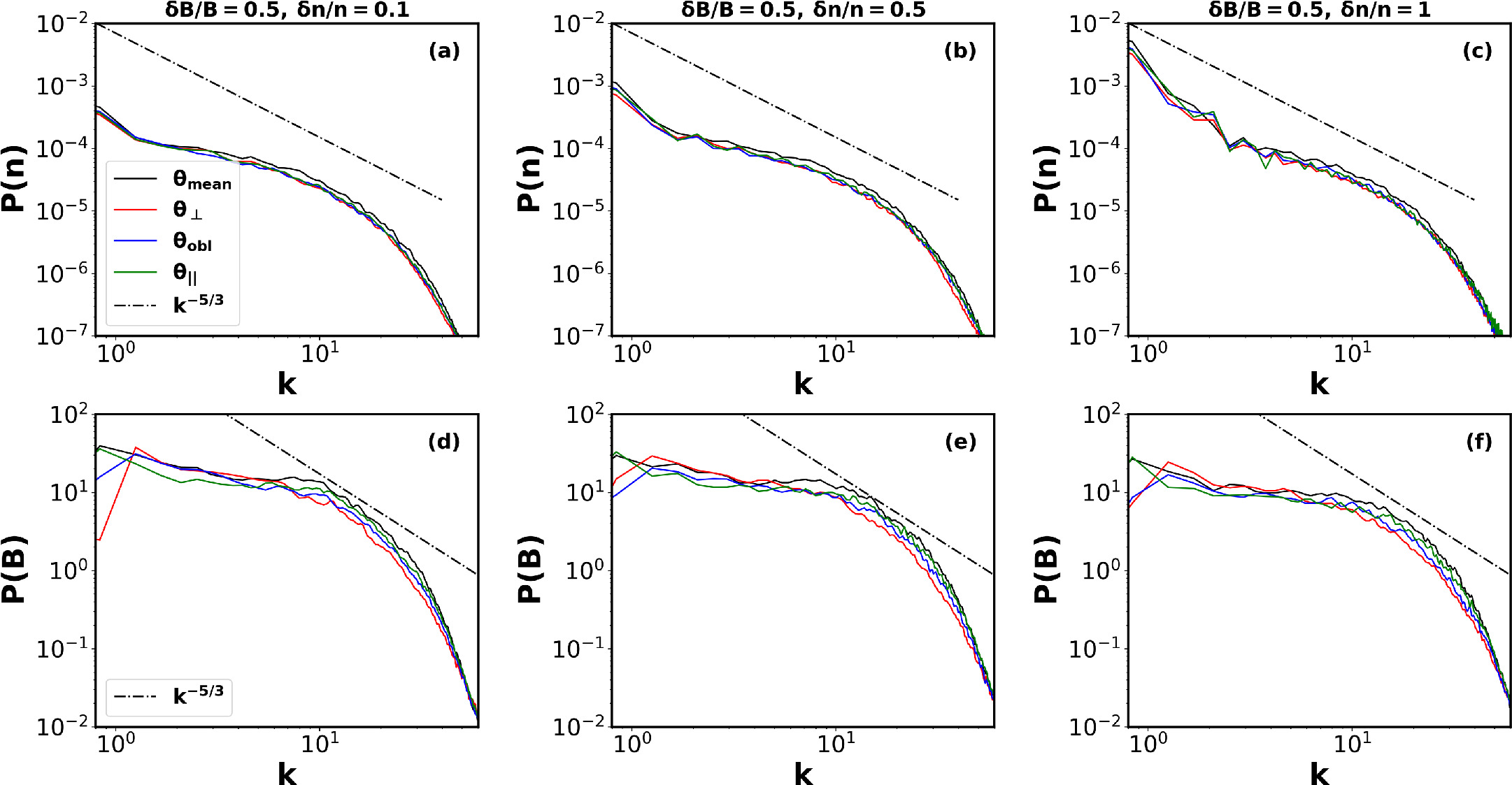
Figure 18. Spectra obtained for Run 4, Run 5, and Run 2.
Download figure:
Standard image High-resolution imageFigures 17 and 18 show analogous results. The density power spectra exhibit a Kolmogorov-type spectrum, and it seems that there is no particular anisotropy because the spectra are completely overlapped. The magnetic field spectra show a different behavior. In order to understand if we are in a regime of fully developed turbulence, we determined the eddy turnover time 60 yr. This implies that the regime of magnetic fully developed turbulence has been reached. This may be related again to the presence of the RTI. Furthermore, the spectra of the three cuts show a slightly anisotropic behavior, as can be seen from the bottom panels in Figures 17 and 18.

3.2. Simulations with Different Mej
We also perform simulations by varying the values of the mass of the ejecta, Mej, to study its effect on the evolution of the SNR. We make a comparison among Run 2, Run 6, and Run 7 (see Table 1). In Figures 19 and 20, we report the spatial maps of the number density, pressure, temperature, the velocity components, and the magnetic field amplitude.

Figure 19. Spatial distribution of the number density, pressure, temperature, x- and y-components of the velocity, and of the magnetic field magnitude from the two-dimensional simulation with an age of 3000 yr for the case Mej = 3 M⊙ (Run 6).
Download figure:
Standard image High-resolution image
Figure 20. Spatial distribution of the number density, pressure, temperature, x- and y-components of the velocity, and of the magnetic field magnitude from the two-dimensional simulation with an age of 3000 yr for the case Mej = 5 M⊙ (Run 7).
Download figure:
Standard image High-resolution imageAt variance with the maps displayed in Figure 3, it is possible to observe that the inner core is denser, especially in the case of 5 Mej (Run 7). This means that as the mass of the ejecta increases, the swept-up time increases. As a consequence, the radius of the FS in Runs 6 and 7 is smaller than in Run 3. In the CD region, the expanding mass interacts with the turbulent and dense ISM environment, but also interacts with an inner dense core. This inhibits the formation of the RTI structures in that region. We further observe a lower magnetic field amplification close to the expanding shock with respect to previous simulations. We found that the magnetic energy and the maximum value reached by the magnetic field within the simulation domain decrease as the mass of the ejecta increases. On the other hand, the kinetic energy increases more slowly in Runs 6 and 7, and consequently the thermal energy decreases more slowly, making the expansion time longer for higher values of Mej. Again, the level of fluctuations is high enough to distort the shock surface and create knots and filaments.
3.3. Simulations with Different Background Densities
We further study the influence of the value of the mean background density on the expansion of the SNR.
When nout = 0.05 cm−3 (Run 8 in Table 1), the SNR expands faster because it interacts with a less dense environment. As a consequence, the FS surface appears to be less distorted and more regular, with the formation of the RTI, as shown in Figure 21(a). In the case of the magnetic field map (Figure 22(a)), strong compression perpendicular to the mean field direction can be noticed, although the magnetic field at the FS is also amplified in small regions all around the shock surface. We underline that such a background density value is close to the one deduced from observations of SN 1006 (F. Acero et al. 2007; G. Morlino et al. 2010). A different behavior is observed in the case of higher ISM densities nout = 1 cm−3 and nout = 3 cm−3. We observe that at a given age of the remnant, the radius of the SNR is smaller and the RTI has not yet completely developed. This is due to the fact that, at the final time, the density values inside and outside the remnant are comparable, thus inhibiting the development of the RTI. Notice the development of magnetic field structures in the ISM that tend to be aligned with the mean magnetic field direction.

Figure 21. Spatial distribution of the number density for Run 8, Run 2, Run 9, and Run 10 with an age of 3000 yr.
Download figure:
Standard image High-resolution image
Figure 22. Spatial distribution of the magnetic field magnitude for Run 8, Run 2, Run 9, and Run 10 with an age of 3000 yr.
Download figure:
Standard image High-resolution imageAlso, in this case, we compare the averaged energies and the magnetic field strength. We find that the magnetic field strength, the magnetic energy, and the kinetic energy associated to the expansion assume higher values when the background density is lower, in agreement with the results shown in F. Guo et al. (2012).
4. Comparison with Chandra Observations
A qualitative comparison between simulations and X-ray observations of SN 1006, as detected by the Chandra spacecraft, has been performed. The X-ray data from Chandra were retrieved from the website.4 Data are provided by the Advanced CCD Imaging Spectrometer instrument on board Chandra, which gives information about the energy, the position, and the arrival time of the X-ray photons. We used observations in the 1.34–3.0 keV energy channel.
The X-ray emission is brighter at the edge of the SN blast wave, and is mainly caused by nonthermal synchrotron emission from relativistic electrons gyrating in an amplified magnetic field. It has been assessed that the brightest cups correspond to regions in which the shock-normal direction is parallel to the direction of the magnetic field (E. M. Reynoso et al. 2013; P. Zhou et al. 2023).
To make a visual comparison between Chandra data and the PLUTO results, we study the degree of anisotropy by applying a ring-shaped mask in a similar way as described in Section 3, but in this case on the brightness field. The results are reported in Figure 23.

Figure 23. (a) Chandra brightness map with the ring-shaped mask overlapped. (b) Autocorrelation function map calculated on the ring-shaped region. The red solid line represents the autocorrelation length, namely the isocontour of C2 = 1/e. (c) Autocorrelation length as a function of angle obtained for Chandra image. (d) Spectra obtained from analysis of the Chandra surface brightness.
Download figure:
Standard image High-resolution imageThe autocorrelation function (Figure 23(b)), similar to the one reported in Figure 7, exhibits the largest values of correlation length along the quasi-perpendicular direction with respect to B0, while the smaller ones lie mainly along the quasi-parallel direction. This can also be deduced by looking at the correlation length reported in Figure 23(c). Thus, magnetic field turbulence decorrelates faster along the mean magnetic field direction. Further investigations need to be carried out in the future, since the analysis performed on the observations does not directly involve the magnetic field, as in the case of numerical simulations. Finally, we also determine the power spectra from the autocorrelation map. We present the three cuts in the autocorrelation map at different angles θ and an omnidirectional spectrum. In Figure 23(d), all the spectra seem to have the same slope, i.e., a Kraichnan slope with k−3/2. Also, in this case, no significant spectral anisotropy has been found within the CD.
5. Conclusions
In this paper, we have tracked the evolution of an SNR using the MHD PLUTO code. Following previous works by D. Balsara et al. (2001), F. Guo et al. (2012), S. Orlando et al. (2012), J. Fang & L. Zhang (2012), and H. Yu et al. (2015), we run a numerical simulation in which an SNR can expand in a turbulent and dense environment. We perform a parametric study, setting up 10 types of simulations, varying the amplitude of the magnetic field fluctuations, the amplitude of the density fluctuations of the ISM, the mass of the ejecta of the SNR, and the value of the background density of the ISM. These can be considered as reference simulations also for comparison with SNR observations. We have analyzed in detail the simulation of an SNR with a mass of the ejecta Mej = 1.4 M⊙ that evolves through an ISM with a level of magnetic fluctuations δB/B = 0.5 and a level of density fluctuations δn/n = 1. The large-scale magnetic field has been oriented within the (x, y) plane using ϕ = 90∘ and = 150∘, which is the orientation deduced from observations of SN 1006 (E. M. Reynoso et al. 2013).

Simulations were run up to a final time of 3000 yr, which corresponds to the Sedov–Taylor phase of an SNR. At this age, we do see the development of the RTI in the CD region. Almost 54% of the initial thermal energy is converted into kinetic energy of the expansion. The presence of a highly turbulent environment favors magnetic field amplification, in particular in the regions perpendicular to the mean magnetic field direction. Indeed, within a highly turbulent ISM, we observe distortion of the shock surface, resulting in the emergence of knots and filaments. We find that, within filamentary regions close to the FS, the magnetic fields are of the order of 100 μG, significantly amplified above the typical ISM value of about 3 μG. Furthermore, the presence of density fluctuations in the ISM leads to the formation of inhomogeneity in the density along the shock front. On the other hand, if the background density of the ISM is particularly high (see Run 10), the expansion of the SNR is slowed down, inhibiting the formation of the RTI within the CD.
Thus, we have investigated the effect of the turbulent environment on the level of anisotropy in the magnetic and density fields within an SNR. This has been achieved using a new technique based on the application of a ring-shaped mask on the region between the RS and the FS to the density and the magnetic field maps. We determine the two-dimensional structure function S2(ℓ) and the autocorrelation function (C(ℓ)) in this ring-shaped region. In order to make a more detailed statistical analysis, we interpolate in polar coordinates the autocorrelation function, from which we extrapolate the correlation length values for fixed angle λc(θ). We also determine the power spectral density at fixed angle values P(k, θ) using the Blackman–Tukey technique. The autocorrelation map suggests in both cases that the correlation scale of turbulence is larger in the direction quasi-perpendicular to B0 and shorter along it. On the other hand, for very low δn/n, isotropy is recovered in the density field within the SNR, since no density inhomogeneities are induced along the shock front. Then, we vary the level of magnetic fluctuations and fix δn/n = 1. While no significant variations are observed in the plasma quantities, the magnetic energy increases as δB/B increases. Thus, we obtain a noticeable amplification of the magnetic field at the shock front (mostly along the perpendicular region) for enhanced ISM turbulence. No significant variations are observed in the other case, in which we vary the level of the density fluctuations and we fix the level of magnetic turbulence to δB/B = 0.5. A small difference is related to the expansion radius of the SN, which decreases as the value of δn/n increases. Since large-amplitude density fluctuations slow down the expansion of the SNR, the remnant is less developed and the magnetic field is less amplified. Another slight difference is observed in the autocorrelation length values, which increase as the values of δn/n become greater.
In simulations in which we varied the mass of the ejecta, we noticed that the radius of the SNR, over a time corresponding to about 3000 yr, is smaller when the mass of the ejecta is higher, since it needs more time to sweep away all the mass initially concentrated in the cylindrical inner core. Further, the RTI is inhibited within the CD. Also, the values of the magnetic energy are smaller when the mass of the ejecta is higher. The maximum value of ∣B∣ behaves in the same manner. The kinetic energy increases at a slower rate as the mass of the ejecta increases. Indeed, when the mass of the ejecta swept up by the inner core is higher, a greater kinetic energy is required in order to wipe out all the mass. This is related to the final time that we chose for the simulations.
Variation of the background density of the ISM causes a change in the expansion rate; indeed, as the background density increases the remnant expands more slowly than in the simulations with low background density. Maps also show that the shock surface is highly distorted because during the expansion the remnant interacts with a very dense environment; as a consequence, the RTI cannot fully develop and the maps show an isotropic behavior.
Finally, we make a preliminary visual comparison between Chandra observations of SN 1006 and numerical simulations. From the brightness map, it is clear that SN 1006 has two bright emitting regions, located on the NE side and in the SW part. These regions are dominated by synchrotron emission from relativistic electrons gyrating around the magnetic field amplified at the shock. Of course, in our PLUTO simulations, we neither take into account the cosmic-ray feedback to the plasma nor any radiation model to mimic the observed radiation at 1–3 keV. We defer the use of the particle-in-cell version of the PLUTO code (A. Mignone et al. 2018; B. Vaidya et al. 2018) to a future work. We have computed the degree of anisotropy as extracted by the Chandra observations, applying a ring-shaped mask to the surface brightness. We find a qualitative good agreement between the autocorrelation maps computed over the SN 1006 brightness and the magnetic and density maps in the PLUTO simulations. The largest correlation length values are located in the region in which the FS is perpendicular to the mean magnetic field direction. Notice that this is not a one-to-one comparison because, on the one hand, the observed and simulated quantities are not the same, and, on the other hand, the inclusion of different factors, such as modeling of the synchrotron radiation (A. M. Bykov et al. 2008; H. Yu et al. 2015; P. F. Velázquez et al. 2017) and the cosmic-ray contribution to the energy conversion, should be taken into account in the simulations.
We have here presented a collection of numerical simulations of an expanding SNR in a turbulent medium, by varying fundamental parameters both in the ISM and within the remnant, in order to evaluate which parameter has a major impact on the SNR evolution. Since in astrophysical systems shock waves propagate in a perturbed medium (M. Neugebauer & J. Giacalone 2005; D. Trotta et al. 2021; M. Nakanotani et al. 2022), setting up a turbulent ISM represents a more realistic choice. In a future work, we plan to extend our simulations to the three-dimensional case, since geometry does affect the magnetic field amplification in filamentary regions close to the FS (Y. Hu et al. 2022); we further plan to include the contribution of cosmic rays in the magnetic field amplification and in the turbulence excitation, in order to make a better and more quantitative comparison with observations of SN 1006.
The results obtained from such simulations can help us in understanding the physical conditions in which SNRs expand in the ISM.
Acknowledgments
G.P. and L.P. acknowledge support by EU FP7 2007–13 through the MATERIA Project (PONa3_00370) and EU Horizon 2020 through the STAR_2 Project (PON R&I2014-20, PIR01_00008) for running the simulations on the "Newton" cluster.
The authors acknowledge compelling discussions with Salvatore Orlando.
C.M. acknowledges the support from the ERC Advanced Grant "JETSET: Launching, propagation and emission of relativistic jets from binary mergers and across mass scales" (grant No. 884631).
The simulations have been performed at the Alarico cluster, at University of Calabria, supported by "Progetto STAR 2-PIR01 00008" (Italian Ministry of University and Research). The authors acknowledge supercomputing resources and support from the ICSC-Centro Nazionale di Ricerca in High Performance Computing, Big Data and Quantum Computing and hosting entity, funded by the European Union – NextGenerationEU.
G.P. acknowledges support by the Italian PRIN 2022, project 2022294WNB, entitled "Heliospheric shocks and space weather: from multispacecraft observations to numerical modeling." Finanziato da Next Generation EU, fondo del Piano Nazionale di Ripresa e Resilienza (PNRR) Missione 4 "Istruzione e Ricerca"—Componente C2 Investimento 1.1, "Fondo per il Programma Nazionale di Ricerca e Progetti di Rilevante Interesse Nazionale (PRIN)".
S.P. acknowledges the project "Data-based predictions of solar energetic particle arrival to the Earth: ensuring space data and technology integrity from hazardous solar activity events" (CUP H53D23011020001), "Finanziato dall" Unione europea – NextGenerationEU, Piano Nazionale di Ripresa e Resilienza (PNRR) Missione 4 "Istruzione e Ricerca"—Componente C2 Investimento 1.1, and "Fondo per il Programma Nazionale di Ricerca e Progetti di Rilevante Interesse Nazionale (PRIN)" Settore PE09.
S.S. and S.P. acknowledge the Space It Up project funded by the Italian Space Agency, ASI, and the Ministry of University and Research, MUR, under contract no. 2024-5-E.0 - CUP n.I53D24000060005.