


Abstract
A H ii region is a kind of emission nebula, and more definite samples of H ii regions can help study the formation and evolution of galaxies. Hence, a systematic search for H ii regions is necessary. The Large Sky Area Multi-Object Fiber Spectroscopic Telescope (LAMOST) conducts medium-resolution spectroscopic surveys and provides abundant valuable spectra for unique and rare celestial body research. Therefore, the medium-resolution spectra of LAMOST are an ideal data source for searching for Galactic H ii regions. This study uses the LAMOST spectra to expand the current spectral sample of Galactic H ii regions through machine learning. Inspired by deep convolutional neural networks with wide first-layer kernels (WDCNN), a new spectral-screening method, multihead WDCNN, is proposed and implemented. Infrared criteria are further used for the identification of Galactic H ii region candidates. Experimental results show that the multihead WDCNN model is superior to other machine-learning methods and it can effectively extract spectral features and identify H ii regions from the massive spectral database. In the end, among all candidates, 57 H ii regions are identified and known in SIMBAD, and four objects are identified as "to be confirmed" Galactic H ii region candidates. The known H ii regions and H ii region candidates can be retrieved from the LAMOST website.
Export citation and abstract BibTeX RIS

Original content from this work may be used under the terms of the Creative Commons Attribution 4.0 licence. Any further distribution of this work must maintain attribution to the author(s) and the title of the work, journal citation and DOI.
1. Introduction
H ii regions, which are chiefly composed of ionized hydrogen atoms, are a kind of emission nebula with massive young stars as the source of ionized photons. These regions appear when massive and young stars ionize neighboring gas clouds with high-energy ultraviolet radiation (Paladini et al. 2004; McQuinn et al. 2007). A H ii region with an approximate temperature of 10,000 K typically contains bright and hot stars and is considered a region of new star formation (O'Dell 2001; Anderson et al. 2009). The shapes of H ii regions are diverse due to the irregular distribution of gas and stars in the H ii region and the ionization of the surrounding gas by the stars within it (Townsley et al. 2006). H ii regions exist in irregular and spiral galaxies and are mostly distributed in the arms of spiral galaxies. Therefore, these regions are the ideal tracers for the spiral structure of the Galaxy (Vallee 1995). The chemical composition of a H ii region is mainly hydrogen, and they also contain a small amount of helium and trace amounts of heavy elements (Shaver et al. 1983). According to their physical size, H ii regions can be divided into six types: hypercompact, ultracompact, compact, classical, giant, and supergiant. Hypercompact, ultracompact, and compact H ii regions represent the early stage of H ii region evolution at which massive stars begin to ionize the interstellar medium around them (Urquhart et al. 2013). The ionizing photons from massive star clusters form supergiant and giant H ii regions, while a few OB stars form other types of H ii regions. The emission of a H ii region at mid- to far-infrared (IR) wavelengths originates from the photodissociation region and the dust within the H ii region (Anderson et al. 2010; Deharveng et al. 2010; Rodón et al. 2010). Transforming the measurement attributes (i.e., angular size and flux) of H ii regions into physical attributes (i.e., physical size and luminosity) requires the H ii region distances, which also play an important role in studying the formation of large-scale Galactic stars and the structure of the Galaxy using the H ii regions (Anderson et al. 2015b). The Galactocentric distances of most known H ii regions are 3–15 kpc (Anderson et al. 2015a). A H ii region, whose evolution begins with a dense large H i cloud, can offer restrictions on the theories of evolution and formation of the Galaxy (Mathews & O'dell 1969; Yorke 1986). The lifespan of a H ii region is approximately several million years (Alvarez et al. 2006). In the final stage of the H ii region evolution, most of the gas is dissipated by the radiation pressure from young and hot stars (Pudritz 2002). The details of massive star formation in H ii regions are currently difficult to completely determine because of the remote distance between the H ii regions and Earth, and that the stars are obscured by dust (Heiles et al. 2000; Straižys et al. 2001; Ward-Thompson et al. 2006).
The Large Sky Area Multi-Object Fiber Spectroscopic Telescope (LAMOST) obtains massive spectra, which provide abundant data for us to find H ii regions. Nevertheless, a planetary nebula (PN) is also an emission nebula consisting of an expanding and glowing shell of ionized gas ejected from red giant stars during the final stages of stellar evolution (Frankowski & Soker 2009); the spectra of a Galactic H ii region and a PN are similar in the optical band. Despite the redshift, they have dominant features, such as Hα 6563Å and O[iii] 4959, 5007 Å (García-Rojas et al. 2005). The main contamination of searching for H ii regions from LAMOST is PNe. However, the number of PNe obtained in the current LAMOST spectra is too small to construct a large known sample. Therefore, PNe may be misjudged as H ii regions when searching for H ii regions by machine learning. Thus, the H ii region candidates obtained should be judged further using other criteria.
The deep echelle spectrophotometry of Galactic H ii regions was proposed by García-Rojas et al. (2006). The Very Large Telescope UV–Visual Echelle Spectrograph collected data at 3100–10400 Å, and over 200 emission lines were discovered in every region. However, the emission lines with high-resolution optical spectra can only be obtained for Galactic H ii regions that are bright. To distinguish H ii regions and PNe, Kniazev et al. (2008) applied a series of classification diagrams and two criteria on the basis of O[iii] 5007/Hβ versus N[ii] 6585/Hα and S[ii] 6718, 6732/Hα. A series of IR color criteria was established by using the data from IR surveys, namely, the Wide-field Infrared Survey Explorer (WISE; Wright et al. 2010), the Spitzer Space Telescope (Werner et al. 2004), to distinguish H ii regions and PNe (Anderson et al. 2012). The combination of optical spectral features and IR color criteria will increase the credibility of the H ii region candidates. In this study, machine learning is implemented to select H ii regions from the massive spectra of LAMOST. The obtained H ii region candidates are crossmatched in WISE and Spitzer, and then the IR color criteria are applied to confirm the final results.
The remainder of this article is organized as follows. Section 2 describes the experimental data, introduces the LAMOST, WISE, and Spitzer databases. Section 3 presents a multihead deep convolutional neural networks with wide first-layer kernels (multihead WDCNN) model, and the use of IR criteria to distinguish H ii regions from PNe. Section 4 provides the experimental results and discussion. Section 5 presents the conclusion and the plans for future work.
2. Data
2.1. LAMOST
LAMOST (Cui et al. 2012; Zhao et al. 2012), also known as the Guoshoujing Telescope, is a reflective Schmitt telescope. This telescope is equipped with 4000 optical fibers and two mirrors, and has a field of view of 5° and a focal length of 20 m. It can simultaneously observe 4000 celestial bodies. It has been used to conduct the medium-resolution spectroscopic (MRS) survey since 2017 September 1, and the latest internal data release is DR11. Each medium-resolution spectrum has two wave bands, namely, the blue band with a wavelength of 4950–5350 Å and the red band with a wavelength of 6300–6800 Å (R ∼ 7500, the limiting magnitude is around G ∼ 15; Zheng et al. 2023). It combines a large aperture with a wide field of view, and has an extremely high spectral acquisition rate for celestial bodies. Moreover, it has been conducting continuous sky surveys to obtain more spectra. It supplies abundant valuable spectra for specific celestial body research, such as Galactic H ii regions. Therefore, the LAMOST spectral database is an ideal data source for searching for the H ii regions.
2.2. WISE
The WISE (Liu et al. 2008) mapped the entire sky at four wavelengths, namely W1, W2, W3, and W4, with respective centers of 3.4, 4.6, 12, and 22 μm, and achieved sensitivity better than 0.08, 0.11, 1, and 6 mJy in the four wave bands observed using conditions such as the low-IR background in space. WISE has increased its sensitivity by using more detectors, and its sensitivity is 1000 times larger than that of the Infrared Astronomical Satellite (IRAS; Mainzer et al. 2005). In our experiment, the 12 μm band of WISE is only applied. The 12 μm band of WISE ought to track homologous dust emission ingredients like the 8.0 μm band of IRAC. However, the 12 μm band is obviously broader than the 8.0 μm band, and the polycyclic aromatic hydrocarbon features at 16.4, 12.7, and 11.2 μm are in this broad band (Tielens 2008). The 12 μm band of WISE saturates for point sources at 0.9 Jy.
2.3. Spitzer
The Spitzer Space Telescope (Werner 2012) uses IRAC instruments to detect the sky at the four wavelengths of 3.6, 4.5, 5.8, and 8 μm, with respective saturation limits of 7.0, 6.5, 4.0, and 4.0 mag. The data from Spitzer, IRAC, and a high-resolution radio continuum indicate that the H ii region is surrounded by a bright 8 μm shell. The termination of the radio continuum at the inner surface of the 8 μm shell indicates that the H ii region is confined by its photodissociation region and the basic coincidence of the radio continuum, and the 24 μm emission line proves that dust exists within the H ii region (Watson et al. 2008). In our experiment, the 8.0 μm band of Spitzer is only used. The properties of this band reduce errors in aperture photometry and facilitate the survey of the source fluxes (Anderson et al. 2012).
2.4. Creation of Training and Test Samples
The WISE catalog of Galactic H ii Regions was created and released by Anderson et al. (2014). To find the H ii regions in the LAMOST data, we crossmatch this WISE catalog of H ii regions with the LAMOST DR9 data within 2'. We obtain 1670 corresponding entries. Considering the spectral quality and obvious characteristics of emission lines, 546 entries are adopted as known H ii regions. Avoiding sample imbalance, the same number of non–H ii regions are selected, as shown in Table 1. Given the small size of known samples, the following experiment adopts k-fold cross validation, where k is 10, to fully utilize the data set and objectively reflect the performance of classification methods.
Table 1. Composition of the Non–H ii Region Sample
| Class | Galaxies | Quasars | Stars | Sky | Other Emission-line Sources |
|---|---|---|---|---|---|
| No. | 109 | 109 | 109 | 109 | 110 |
Download table as: ASCIITypeset image
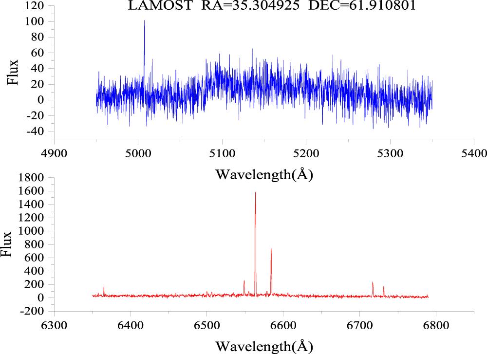
We take two Galactic H ii region spectra from the LAMOST as an example, as illustrated in Figure 1. The fluxes of LAMOST spectra are displayed in instrumental units as they are not calibrated.
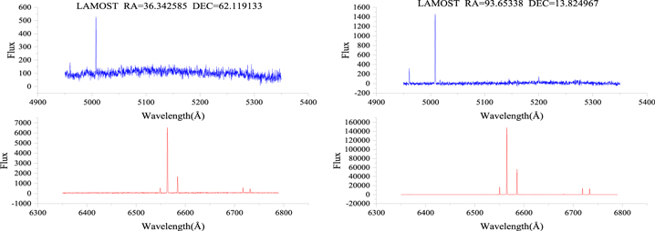
Figure 1. LAMOST spectra of two Galactic H ii regions. The upper panels are part of the blue wavelength, and the lower panels are part of the red wavelength.
Download figure:
Standard image High-resolution image3. Method
3.1. Multihead WDCNN Model
Machine learning is widely used in processing massive astronomical data sets (Ball & Brunner 2010; Bloom & Richards 2012). Its ability to classify spectra and its accuracy and efficiency are usually higher than those of manual classification. Two-dimensional CNN usually uses 3 × 3 or 5 × 5 convolution kernels (Simonyan & Zisserman 2014; Krizhevsky et al. 2017; Szegedy et al. 2017; Wu et al. 2019). A small-sized convolution kernel can obtain the same receptive field with fewer parameters than a large-sized convolution kernel. The use of small-sized convolution kernels suppresses the overfitting caused by too many parameters and increases the depth of the network due to the use of more convolution kernels. However, small convolution kernels need to obtain the same receptive field through more parameters for 1D CNN (Zhang et al. 2018).
Inspired by WDCNN (Zhang et al. 2017), this paper proposes multihead WDCNN. Using multiple convolution kernels of different sizes on the same feature map is an effective way of improving the model's ability to extract features (Szegedy et al. 2015; Das et al. 2020; Wu et al. 2023). The network structure is shown in Figure 2. On the basis of WDCNN, 64 × 1 is replaced with 32 × 1, 64 × 1, and 128 × 1 three large-sized convolution kernels to improve the extraction of features of different sizes. The multihead WDCNN model is superior to WDCNN with higher classification accuracy, and can single out H ii regions more correctly from massive LAMOST spectra.
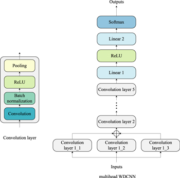
Figure 2. Structural diagram of the multihead WDCNN model.
Download figure:
Standard image High-resolution image3.2. IR Classification Criteria
H ii regions and PNe are easily mistaken for each other, but IR images are helpful in discriminating them (Cohen et al. 2007, 2011). Aperture photometry is a photometric method that calculates the flux of a target object in a certain band by summing the flux in an aperture centered on the target object and subtracting the background flux (Mighell 1999). The 12 μm IR image provided by the WISE satellite and the 8 μm IR image provided by the Spitzer space telescope are required to distinguish H ii regions and PNe through aperture photometry. First, the aperture photometry method is used to obtain the flux of the target celestial body in the two IR bands of 12 and 8 μm; then, the category of the target celestial body is further confirmed by the IR color criteria (Anderson et al. 2012). Since H ii regions and PNe display similar features in optical wavelengths, after using the multihead WDCNN model to obtain H ii region candidates from the massive spectra, they may contain PNe that are mistakenly considered as H ii regions. However, H ii regions and PNe can be distinguished by their IR colors, so the IR criteria can be used after applying the multihead WDCNN model. Table 2 shows the established IR color criteria for distinguishing H ii regions and PNe, where the brackets indicate a base 10 logarithm, and Fλ is the IRAS flux at wavelength λ.
Table 2. IR Color Criteria for H ii Regions
| Criteria | References |
|---|---|
| [F25/F12] ≥ 0.57, [F60/F12] ≥ 1.30 | Wood & Churchwell (1989) |
| [F25/F12] ≥ 0.4, [F60/F12] ≥ 0.25 | Hughes & MacLeod (1989) |
| [F160/F24] > 0.8 (or [F160/F22] > 0.8) | Anderson et al. (2012) |
| [F160/F12] > 1.3 | Anderson et al. (2012) |
| [F12/F8] < 0.3 | Anderson et al. (2012) |
Download table as: ASCIITypeset image
[F160/F24] > 0.8 (or [F160/F22] > 0.8), [F160/F12] > 1.3, and [F12/F8] < 0.3 are the most reliable discriminating color criteria. We use the Kang software and Equation (1) to perform aperture photometry on the unrecorded H ii regions in the Set of Identifications, Measurements, and Bibliography for Astronomical Data (SIMBAD; Anderson et al. 2012)

where Sν at the left side of the equation refers to the source flux after background correction, Sν,0 at the right side of the equation points to the source flux without background correction, Bν represents the flux in the background aperture, NB describes the number of pixels in the background aperture, and NS is the number of pixels in the source aperture. A single source aperture and four background apertures were defined in our experiment. The process subtracts the average flux in the background apertures from each pixel in the source aperture. The WISE image data have digital numbers (DN) units, and we use the DN-to-Jy conversion factor of 2.9045 × 10⁻⁶ for the 12 μm band. The Spitzer image data have MJy sr−1 units, and we adopt the MJy sr−1-to-Jy conversion factor of 8.461595 × 10⁻⁶ for the 8 μm band (Anderson et al. 2012).
3.3. The Schema of the Experiment
The overall process of this experiment is shown in Figure 3. The process is divided into the following three steps:
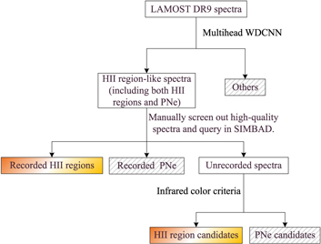
Figure 3. Experimental flowchart.
Download figure:
Standard image High-resolution imageStep 1: Train a network model (multihead WDCNN) and apply it to automatically and efficiently select H ii region–like spectra in the LAMOST medium-resolution spectra. It is a rough screening rather than distinguishing between H ii regions and PNe since the spectra of H ii regions are similar to those of PNe.
Step 2: These spectra predicted to be H ii region–like require manual screening to obtain high-quality spectra. Query the results obtained in SIMBAD with a search range of 2', and for the recorded H ii regions we may supplement the medium-resolution spectra with the H ii region spectral library.
Step 3: For the unrecorded spectra in SIMBAD, we further confirm them through the IR color criteria and label them as H ii region candidates or PNe candidates.
Table 3. Detailed Parameters of the Multihead WDCNN Model when the Size of the Input Data is 6284 × 1
| Layer Type | Kernel Size/Stride | Kernel Number | Output Size (Width × Depth) | Padding |
|---|---|---|---|---|
| Convolution 1_1 | 32 × 1/8 × 1 | 16 | 783 × 16 | 2 |
| Pooling 1_1 | 2 × 1/2 × 1 | 16 | 392 × 16 | 1 |
| Convolution 1_2 | 64 × 1/16 × 1 | 16 | 390 × 16 | 2 |
| Pooling 1_2 | 2 × 1/2 × 1 | 16 | 195 × 16 | 0 |
| Convolution 1_3 | 128 × 1/32 × 1 | 16 | 194 × 16 | 10 |
| Pooling 1_3 | 2 × 1/2 × 1 | 16 | 97 × 16 | 0 |
| Convolution 2 | 3 × 1/1 × 1 | 32 | 684 × 32 | 1 |
| Pooling 2 | 2 × 1/2 × 1 | 32 | 342 × 32 | 0 |
| Convolution 3 | 3 × 1/1 × 1 | 64 | 342 × 64 | 1 |
| Pooling 3 | 2 × 1/2 × 1 | 64 | 171 × 64 | 0 |
| Convolution 4 | 3 × 1/1 × 1 | 64 | 171 × 64 | 1 |
| Pooling 4 | 2 × 1/2 × 1 | 64 | 86 × 64 | 1 |
| Convolution 5 | 3 × 1/1 × 1 | 64 | 84 × 64 | 0 |
| Pooling 5 | 2 × 1/2 × 1 | 64 | 42 × 64 | 0 |
| Linear 1 | 100 | 1 | 100 × 1 | |
| Linear 2 | 2 | 1 | 2 × 1 |
Download table as: ASCIITypeset image
4. Experimental Results and Discussion
Since the LAMOST spectra are not flux calibrated, we normalize the spectra before training a model. The 4950–5350 Å blue band and the 6350–6790 Å red band must be subjected to min–max normalization separately before using them in the neural network, as shown in Equation (2). Then, these bands should be spliced into 1D data with a single data size of 6284 × 1. The parameters of the multihead WDCNN model are illustrated in Table 3 with the input data size of 6284 × 1.

Table 4. The Average Accuracy of Five Models on the LAMOST Spectra
| Classifier | SVM (poly) | RF (100) | ANN (Default) | WDCNN | Multihead WDCNN |
|---|---|---|---|---|---|
| Accuracy (%) | 86.85 ± 4.33 | 85.83 ± 5.12 | 88.61 ± 4.75 | 92.12 ± 3.07 | 92.68 ± 2.99 |
Download table as: ASCIITypeset image
The control group of this experiment uses three traditional machine-learning methods: support vector machine (SVM; Cortes & Vapnik 1995), random forest (RF; Breiman 2001), and artificial neural network (ANN; Jeffrey & Rosner 1986). These three methods are implemented with the sklearn library in which two groups of SVM use "poly" and "rbf" nonlinear kernel functions, eight groups of RF use eight different numbers of basic learners (from 50 to 400, with a step size of 50), and ANN is implemented with a multilayer perceptron and its model parameters are set as default values. The results of the 10-fold cross validation of the five classification methods on the known H ii region and non–H ii region samples are shown in Table 4. For SVM and RF, we only keep the best result in Table 4. As described in Table 4, the multihead WDCNN model has a higher classification accuracy (92.68%) and a smaller standard deviation (2.99%) than the other models (SVM, RF, ANN, and WDCNN).
The multihead WDCNN model outperforms other classifiers, so we use the trained multihead WDCNN model to select H ii regions from the released LAMOST MRS database. This model is used for preliminary screening. The H ii region candidates singled out need be manually checked, poor-quality spectra due to low signal-to-noise ratio and other reasons eliminated by manual inspection, and the remaining spectra identified step by step with SIMBAD and IR criteria. Finally 57 recorded H ii regions are found in SIMBAD, as shown in the

Figure 4.
The upper blue spectra are the blue band part of LAMOST, and the lower red spectra are the red band part of LAMOST. (The complete figure set (57 images) is available.)
Download figure:
Standard image High-resolution image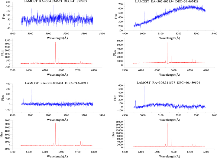
Figure 5. LAMOST spectra of H ii region candidates. The upper blue spectra are the blue band part of LAMOST, and the lower red spectra are the red band part of LAMOST.
Download figure:
Standard image High-resolution image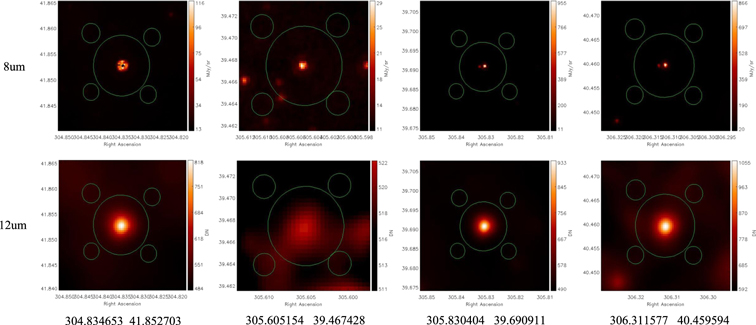
Figure 6. Aperture photometry process.
Download figure:
Standard image High-resolution image
Table 5. Aperture Photometry Results
| R.A. | Decl. | GLON | GLAT | Rad (') | F12 (Jy) | F8 (Jy) | [F12/F8] |
|---|---|---|---|---|---|---|---|
| 304.834653 | 41.852703 | 79.156164 | 3.220179 | 1.5 | 0.091975 | 0.091531 | 0.002102 |
| 305.605154 | 39.467428 | 77.521212 | 1.38647 | 0.7 | 0.001842 | 0.004624 | −0.399728 |
| 305.830404 | 39.690911 | 77.80391 | 1.371859 | 2 | 0.130807 | 0.290542 | −0.346578 |
| 306.311577 | 40.459594 | 78.644797 | 1.512536 | 1.6 | 0.159614 | 0.315833 | −0.296387 |
Download table as: ASCIITypeset image
In general, confirming a Galactic H ii region is challenging and complicated. A sight line through a large H ii region may be far from the H ii region's centroid and not return a match in SIMBAD and the criterion adopted in a previous study (Anderson et al. 2012). [F12/F8] < 0.3 can only meet 98% of the H ii regions and ∼10% of PNe. Multiple spectra can originate from the same region, and a spectrum may display characteristics of a H ii region but originate from diffuse ionized gas. Therefore, the final four candidates are called "to be confirmed" candidates rather than definite H ii regions, requiring further verification. The IR images in Figure 6 are provided for visual inspection.
5. Conclusion
Experiments show that large-sized convolution kernels can achieve improved results when using convolution kernels to extract the features of 1D data for the first time. Combining multiple large convolution kernels with different sizes can decrease the randomness of the model during training and slightly improve the classification performance. The multihead WDCNN model is improved on the basis of the WDCNN model. The convolution kernel with a length of 64 in the first convolution layer of the original model is replaced by three convolution kernels with lengths of 32, 64, and 128 to improve the extraction of features of different sizes. We used this method to obtain Galactic H ii regions from the LAMOST medium-resolution spectra. LAMOST is conducting an unprecedented MRS survey that will provide more detailed information that is critical for the research of the properties of H ii regions. In future work, we will further identify the unrecorded H ii regions and add them to the present H ii region spectral library. These spectra can be used to enlarge the H ii region training sample. With the increase of known H ii regions, we will retrain the multihead WDCNN model and more H ii region spectra will be discovered with the successive release of the medium-resolution spectra of LAMOST.
Acknowledgments
We are very grateful to the referee's constructive report for helping us to improve our paper. We would like thank Dr. L. D. Anderson for providing the Kang software and guiding us on its usage for aperture photometry. This work was funded by the National Natural Science Foundation of China under grant Nos. 12273076, 12133001, and 11873066, the science research grants from the China Manned Space Project with Nos. CMS-CSST-2021-A04 and CMS-CSST-2021-A06, and the Natural Science Foundation of Hebei Province No. A2018106014. Guoshoujing Telescope (LAMOST) is a national major scientific project of the Chinese Academy of Sciences. Funding for the project was provided by the National Development and Reform Commission. We acknowledge the use of the spectra from LAMOST. This research used SIMBAD and the WISE and Spitzer databases.
Appendix: Search Results of H ii Regions in SIMBAD
The 57 H ii regions recorded in SIMBAD are indicated in Table 6.
Table 6. Search Results of H ii Regions in SIMBAD
| R.A. | Decl. | GLON | GLAT | SIMBAD Name | Dist. (arcseconds) | References |
|---|---|---|---|---|---|---|
| (1) | (2) | (3) | (4) | (5) | (6) | (7) |
| 35.304925 | 61.910801 | 133.289494 | 0.858016 | LBN 133.27+00.82 | 100.88 | None |
| 36.330775 | 62.069134 | 133.686375 | 1.173764 | W 3j | 61.33 | 1 ∼ 11 |
| 36.342585 | 62.119133 | 133.673809 | 1.222474 | GAL 133.69+01.22 | 43.64 | None |
| 36.403928 | 62.052467 | 133.724342 | 1.170353 | W 3k | 64.52 | 12 ∼ 14 |
| 36.742716 | 61.877464 | 133.935713 | 1.063954 | GAL 133.938+01.066 | 12.39 | 15 |
| 36.794904 | 61.885799 | 133.955649 | 1.080601 | MSX6C G133.9476+01.0648 | 63.75 | 16 ∼ 17 |
| 36.797319 | 62.202465 | 133.842307 | 1.376300 | LBN 133.82+01.38 | 79.91 | None |
| 41.854501 | 61.910801 | 136.133681 | 2.048857 | SH 2-192 | 11.56 | 18 ∼ 29 |
| 41.929559 | 61.977467 | 136.136704 | 2.124233 | SH 2-193 | 21.97 | 30 ∼ 31 |
| 42.299335 | 60.769131 | 136.822254 | 1.113364 | IRAS 02455+6034 | 98.49 | 32 ∼ 42 |
| 42.875048 | 62.219131 | 136.428299 | 2.535654 | SH 2-196 | 37.42 | 43 ∼ 51 |
| 45.428187 | 60.494133 | 138.312230 | 1.572605 | [KCW94] 138.300+01.558 | 66.83 | 52 ∼ 56 |
| 45.813204 | 60.469131 | 138.490576 | 1.642093 | SH 2-201 | 25.93 | 57 ∼ 74 |
| 60.807833 | 51.298603 | 150.600009 | −0.966664 | NGC 1491 | 61.99 | 75 ∼ 116 |
| 60.977297 | 51.306617 | 150.674141 | −0.890536 | LBN 150.69-00.90 | 56.41 | None |
| 79.04976 | 34.3198 | 172.062826 | −2.272305 | [ABB2014] G172.080-02.258 | 82.81 | 117 |
| 80.77818 | 33.9705 | 173.168606 | −1.299337 | IRAS 05197+3355 | 2.48 | 118 ∼ 126 |
| 80.77967 | 33.4755 | 173.577798 | −1.578074 | [AAJ2015] G173.581-01.577 | 16.66 | 30,117 |
| 85.247667 | 35.846239 | 173.602743 | 2.794458 | GAL 173.60+02.80 | 17.81 | 127 ∼ 131 |
| 90.982618 | 30.22129 | 180.899028 | 4.085358 | LBN 181.00+04.13 | 93.83 | 132 |
| 91.023506 | 30.256883 | 180.885124 | 4.133548 | SH 2-241 | 25.23 | 133 ∼ 138 |
| 92.18298 | 15.702592 | 194.124067 | −2.024083 | NAME Lower's Nebula | 99.36 | 139 ∼ 156 |
| 92.200492 | 21.627075 | 188.948883 | 0.861339 | [KC97c] G189.0+00.9 | 57.07 | 131 |
| 92.21332 | 15.715278 | 194.127098 | −1.992385 | LBN 194.20-01.99 | 38.8 | 117 |
| 92.251298 | 20.640514 | 189.834908 | 0.424751 | SH 2-252 B | 30.02 | 157 ∼ 164 |
| 92.73015 | 20.60315 | 190.084196 | 0.79907 | IRAS 06078+2037 | 36.17 | 117 |
| 93.65338 | 13.824967 | 196.455066 | −1.679042 | IRAS 06117+1350 | 6.7 | 165 ∼ 180 |
| 93.962301 | 14.277395 | 196.200008 | −1.199997 | [AAL2018] G196.206-01.183 | 64.91 | 181 |
| 96.428671 | 19.998551 | 192.257942 | 3.570344 | SH 2-253 | 97.26 | 182 ∼ 186 |
| 98.157199 | 6.993974 | 204.566115 | −0.967991 | [C51] 141 | 117.12 | 29 |
| 98.39939 | 4.79414 | 206.629914 | −1.768324 | GAL 206.618-01.8 | 81.36 | 129 |
| 98.58245 | 2.498597 | 208.754113 | −2.661352 | [AAL2018] G208.741-02.633 | 112.43 | 117 |
| 98.65856 | 2.477611 | 208.807709 | −2.603423 | [C51] 142 | 50.0 | 29 |
| 99.049625 | 10.866667 | 201.534349 | 1.598109 | [ABB2014] G201.535+01.597 | 4.64 | 117 |
| 99.176521 | 10.777308 | 201.671002 | 1.667831 | GAL 201.6+01.6 | 89.74 | 187 ∼ 194 |
| 99.225618 | 11.960641 | 200.640836 | 2.253155 | [C51] 143 | 98.01 | 29 |
| 100.15054 | 9.802307 | 202.977246 | 2.073533 | [ABB2014] G202.968+02.083 | 47.61 | 117 |
| 100.29393 | 9.602307 | 203.21988 | 2.10794 | [KC97c] G203.2+02.1 | 96.82 | 131 |
| 101.27076 | 6.61064 | 206.324843 | 1.603512 | LBN 206.29+01.55 | 83.53 | 140 |
| 304.702911 | 40.796593 | 78.226059 | 2.70795 | DWB 65 | 104.91 | 195 ∼ 196 |
| 305.207622 | 39.575137 | 77.435227 | 1.699916 | [AAJ2015] G077.435+01.703 | 11.13 | 30 |
| 305.603424 | 40.228477 | 78.1456 | 1.821953 | [KC97c] G078.1+01.8 | 22.08 | 128 |
| 305.755219 | 41.556637 | 79.302251 | 2.486209 | [AAJ2015] G079.294+02.491 | 34.28 | 30 |
| 305.774719 | 40.096462 | 78.112053 | 1.639086 | DWB 62 | 82.85 | 196 |
| 306.221435 | 40.424938 | 78.576902 | 1.548606 | DWB 77 | 90.77 | 196 |
| 306.477387 | 40.017013 | 78.356628 | 1.153507 | DWB 70 | 85.69 | 197 |
| 306.525574 | 40.504894 | 78.775879 | 1.405888 | LBN 078.73+01.45 | 72.16 | None |
| 307.032074 | 40.018021 | 78.604344 | 0.808376 | LBN 078.55+00.85 | 109.65 | 198 |
| 312.930555 | 44.20258 | 84.587198 | −0.102069 | [C51] 75 | 85.55 | 29 |
| 344.07164 | 58.521664 | 108.365291 | −1.055093 | SH 2-149 | 5.35 | 199 ∼ 217 |
| 346.26225 | 60.26068 | 110.100008 | 0.066667 | [UHP2009] VLA G110.1081+00.0478 | 73.93 | 218 |
| 346.292299 | 60.24522 | 110.107528 | 0.046548 | SH 2-156 A | 3.8 | 219 ∼ 222 |
| 348.40409 | 61.4878 | 111.533342 | 0.800001 | [WBN74] NGC 7538 IRS 4 | 32.92 | 223 ∼ 238 |
| 348.851278 | 59.926484 | 111.166675 | −0.733333 | [C51] 102 | 95.7 | 29 |
| 349.19833 | 61.916073 | 112.039662 | 1.062453 | [AAL2018] G112.029+01.050 | 58.97 | 181 |
| 350.104932 | 61.175469 | 112.184428 | 0.217412 | [KC97c] G112.2+00.2a | 21.68 | 131 |
| 358.264221 | 60.494152 | 115.800009 | −1.566665 | LBN 115.84-01.60 | 32.83 | None |
Note. Column (3): Galactic longitude. Column (4): Galactic latitude. Column (5): Name of H ii region in SIMBAD. Column (6): Distance from observed source in LAMOST to H ii region recorded in SIMBAD. Column (7): Related references: (1) Bik et al. (2012); (2) Feigelson & Townsley (2008); (3) Ojha et al. (2006); (4) Schleuning et al. (2000); (5) Garay & Lizano (1999); (6) Normandeau (1999); (7) Tieftrunk et al. (1997); (8) Roberts et al. (1993); (9) van der Werf & Goss (1990); (10) Dickel et al. (1983); (11) Colley (1980); (12) Kiminki et al. (2015); (13) Han & Zhang (2007); (14) Sullivan & Downes (1973); (15) Harten (1976); (16) Maud et al. (2015b); (17) Maud et al. (2015a); (18) Foster & Brunt (2015); (19) Sreenilayam & Fich (2011); (20) Azimlu & Fich (2011); (21) Qin et al. (2008); (22) Russeil et al. (2007); (23) Chan & Fich (1995); (24) Fich (1993); (25) Fich et al. (1990); (26) Avedisova & Palous (1989); (27) Fich & Blitz (1984); (28) Blitz et al. (1982); (29) Dubout-Crillon (1976); (30) Anderson et al. (2015a); (31) Kronberger et al. (2006); (32) Liu et al. (2010); (33) Karr & Martin (2003); (34) Szymczak & Kus (2000); (35) Carpenter et al. (2000); (36) Szymczak et al. (2000); (37) Wu et al. (1999); (38) Slysh et al. (1999); (39) Wu et al. (1998); (40) Lyder & Galt (1997); (41) Shepherd & Churchwell (1996); (42) Bronfman et al. (1996); (43) Ginsburg et al. (2011); (44) Hunter (1992); (45) Hunter et al. (1990); (46) Hunter & Massey (1990); (47) Braunsfurth (1983); (48) Felli & Harten (1981); (49) Rohlfs et al. (1977); (50) Georgelin & Georgelin (1976); (51) Churchwell & Felli (1970); (52) Deharveng et al. (2012); (53) Koenig et al. (2008); (54) Hanson et al. (2002); (55) Zapata et al. (2001); (56) Kurtz et al. (1994); (57) Zhang et al. (2021); (58) Eswaraiah et al. (2020); (59) Bobotsis & Fich (2019); (60) Samal et al. (2018); (61) Samal et al. (2012); (62) Balser et al. (2011); (63) Nakano et al. (2008); (64) Kothes & Kerton (2002); (65) Omar et al. (2002); (66) Comerón & Torra (1999); (67) Chen et al. (1995); (68) Sato (1990); (69) Mampaso et al. (1989); (70) Lockman (1989); (71) Burov et al. (1988); (72) Felli et al. (1987);(73) Mampaso et al. (1987); (74) Dickinson et al. (1974); (75) Winston et al. (2020); (76) Luisi et al. (2020); (77) Luisi et al. (2019); (78) Balser & Bania (2018); (79) Fernández-Martín et al. (2017); (80) Wenger et al. (2013); (81) Acker et al. (2012); (82) Romero & Cappa (2009); (83) Bania et al. (2007); (84) Foster et al. (2006); (85) Balser (2006); (86) Rudolph et al. (2006); (87) Pilyugin et al. (2003); (88) Bania et al. (2002); (89) Pilyugin (2001); (90) Inoue et al. (2001); (91) Ghosh et al. (2000); (92) Langston et al. (2000); (93) Ghosh (2000); (94) Peña et al. (2000); (95) Balser et al. (1999); (96) Mookerjea et al. (1999); (97) Rood et al. (1998); (98) Bania et al. (1997); (99) Bell (1995); (100) Balser et al. (1995); (101) Balser et al. (1994); (102) Rubin et al. (1988); (103) Schwartz (1987); (104) Bania et al. (1987); (105) Albert et al. (1986); (106) Fich (1986); (107) Abramenkov (1985); (108) Wink et al. (1983); (109) Thum & Nishimura (1983); (110) Price et al. (1983);(111) Icke et al. (1980); (112) Mezger et al. (1979); (113) Churchwell et al. (1978); (114) Israel (1977); (115) Lo & Burke (1973); (116) Gebel (1968); (117) Wang et al. (2018); (118) Lundquist et al. (2014); (119) Litovchenko et al. (2011); (120) Fontani et al. (2010); (121) Deharveng et al. (2005); (122) Henning et al. (1992); (123) Palla et al. (1991); (124) Wouterloot & Brand (1989); (125) Richards et al. (1987); (126) Casoli et al. (1986); (127) Kirsanova et al. (2020); (128) Lee et al. (2012); (129) Quireza et al. (2006); (130) Conti & Crowther (2004); (131) Kuchar & Clark (1997); (132) Lee et al. (1999); (133) Gao et al. (2019); (134) Figueira et al. (2017); (135) Pomarès et al. (2009); (136) Vilchez & Esteban (1996); (137) Fich & Silkey (1991); (138) Moffat et al. (1979); (139) Gao & Han (2013); (140) Gao et al. (2011); (141) Hausen et al. (2002); (142) Reynolds et al. (2001); (143) Kawamura et al. (1998); (144) Lockman et al. (1996); (145) Carpenter et al. (1995); (146) Garnett (1989); (147) Reynolds (1988); (148) Krymkin & Sidorchuk (1988); (149) Chavarria-K. et al. (1987); (150) Reynolds (1985); (151) Caswell (1985); (152) Garay & Rodriguez (1983); (153) Pismis & Hasse (1982); (154) Hawley (1978); (155) Roberts (1972); (156) Georgelin (1970); (157) Jose et al. (2013); (158) Jose et al. (2012); (159) Minier et al. (2000); (160) Haikala (1995); (161) Koempe et al. (1989); (162) Chavarria-K. et al. (1989); (163) Haikala (1986); (164) Felli et al. (1977); (165) Purser et al. (2021); (166) Quiroga-Nuñez et al. (2019); (167) Ruiz-Velasco et al. (2016); (168) Sawada-Satoh et al. (2013); (169) Jiang et al. (2003); (170) Lekht et al. (2001); (171) Deharveng et al. (2000); (172) Harju et al. (1998); (173) Baudry et al. (1997); (174) Godbout et al. (1997); (175) Eiroa & Casali (1995); (176) Eiroa et al. (1994); (177) Zavagno et al. (1992); (178) Pismis & Mampaso (1991); (179) Wouterloot et al. (1988); (180) Wynn-Williams et al. (1974); (181) Anderson et al. (2018); (182) Daflon et al. (2007); (183) Daflon & Cunha (2004); (184) Daflon et al. (2004);(185) Brand & Blitz (1993); (186) Fich et al. (1989); (187) Semenova et al. (2009); (188) Dickinson et al. (2007); (189) Dickinson et al. (2006); (190) Watson et al. (2005); (191) Finkbeiner et al. (2004); (192) Finkbeiner et al. (2002); (193) McCullough & Chen (2002); (194) Shaver et al. (1983); (195) Higgs et al. (1991); (196) Dickel et al. (1969); (197) Wendker (1970); (198) Odenwald & Schwartz (1993); (199) Li et al. (2022); (200) Dutta et al. (2018); (201) Sreenilayam et al. (2014); (202) Tian et al. (2010); (203) Scaife et al. (2008); (204) Kerton (2006); (205) Kothes et al. (2002); (206) Caplan et al. (2000); (207) Smutko & Larkin (1999); (208) Deharveng et al. (1999); (209) Mirzoyan et al. (1994); (210) Pismis (1990); (211) Lozinskaia et al. (1986); (212) Tatematsu et al. (1985); (213) Wramdemark (1981); (214) Pismis & Hasse (1980); (215) Recillas-Cruz & Pismis (1979); (216) Blitz (1979); (217) Glushkov et al. (1975); (218) Urquhart et al. (2009); (219) Galliano et al. (2008); (220) Dale et al. (2006); (221) Morisset (2004); (222) Giveon et al. (2002); (223) Sandell et al. (2020); (224) Binder & Povich (2018); (225) Sharma et al. (2017); (226) Mallick et al. (2014); (227) Puga et al. (2010); (228) Barriault & Joncas (2007); (229) Kraus et al. (2006); (230) Pestalozzi et al. (2006); (231) Ojha et al. (2004); (232) Sandell & Sievers (2004); (233) Lebrón et al. (2001); (234) Zheng et al. (2001); (235) Yao & Shuji (1999); (236) Akabane et al. (1992); (237) Tamura et al. (1991); (238) Deharveng et al. (1979).