


Abstract
The Atacama Large Millimeter/submillimeter Array high-frequency long-baseline campaign in 2019 (HF-LBC-2019) was arranged to undertake band 9 (690 GHz) and 10 (850 GHz) observations using the longest 16 km baselines in order to explore calibration feasibility and imaging capabilities. Observations were arranged using close calibrators between 0° and 4° from the target point-source quasars (QSOs) to also explore subtle effects of calibrator separation angle. A total of 13 observations were made, five using standard in-band observations and eight using the band-to-band (B2B) observing mode, where phase solutions are transferred from a lower frequency band. At bands 9 and 10, image angular resolutions as high as 7 and 5 mas were achieved, respectively. Both in-band and B2B experiments were successful in imaging the target QSOs but with varying degrees of quality. Target image coherence varied between 0.14 and 0.79, driven by the calibrator separation angle and effectiveness of phase referencing despite observing in correct stability conditions. We conclude that the phase rms conditions and calibrator selection, specifically separation angle from the target, must carefully be considered prior to observing in order to minimize imaging defects. For bands 9 and 10, in order to achieve a coherence >0.7 such that the image structure and source flux can be regarded as suitably accurate, a 1° separated calibrator should be used while the phase rms over the phase switching cycle time should ideally be <30°.
Export citation and abstract BibTeX RIS

Original content from this work may be used under the terms of the Creative Commons Attribution 4.0 licence. Any further distribution of this work must maintain attribution to the author(s) and the title of the work, journal citation and DOI.
1. Introduction
Long-baseline observations (∼16.2 km) with the Atacama Large Millimeter/submillimeter Array (ALMA) at the highest frequency bands (band 9: 602−720 GHz, and band 10: 787−950 GHz) are one of the remaining modes yet to be fully offered for principal investigator (PI) science. The first ALMA long-baseline observations in bands 3, 4, and 6 were highlighted by ALMA Partnership et al. (2015a, 2015c,2015d) and since 2015, ALMA has been observing with long baselines at these bands (and shortly thereafter band 5). Following from the aforementioned investigations, further studies were conducted to explore the long-baseline capability at higher frequencies (Asaki et al. 2020a, 2020b; Maud et al. 2020, 2022), which played a key role in Cycle 7 being the first to offer band 7 (273-373 GHz) long-baseline observations where resolutions of 15–20 mas were achievable. Only very recently for ALMA Cycle 9 (starting 2022 October), as a result of the high-frequency long-baseline campaign 2019 (HF-LBC-2019) data we publish here, ALMA opened band 8 observations with 16 km baselines, while slightly extending the array configurations for band 9 and band 10 to use maximal baselines of 13.9 km and 8.5 km, respectively. These modes offered for the first time ∼10 mas angular resolutions.
As a high priority for the Extension and Optimization of Capabilities (see also Maud et al. 2021), a part of the ObsMode process (Takahashi et al. 2021), the HF-LBC 2019 was arranged to piece together the requirements before offering any high-frequency (band 8, 9 and 10) modes at the longest baselines publicly. Such long-baseline observations at the highest frequencies in band 10 will be able to realize angular resolutions as high as 5 mas. In the scope of the recent high spatial resolution observations with ALMA and the possible detections of circumplantetary disks around protostars (e.g., Tsukagoshi et al. 2019; Benisty et al. 2021), the new mode would offer up to 6 times better angular resolution. Indeed, it is thought possible to image and spatially resolve circumplanetary disks around massive planets within protoplanetary disks (Isella et al. 2019; Tsukagoshi et al. 2019). Considering the recent surveys such as DSHARP (Andrews et al. 2018, 2021) and MAPS (Öberg et al. 2021), the resolution achievable for new high-frequency long baselines would be sub−astronomical unit scales, between ∼5 and 20 times better angular resolution than any observations to date, and could therefore provided an unprecedented view of the rings and spiral arm features around these protostars. ALMA is the only instrument that will currently offer such angular resolution, although some specific observations may be difficult due to optical depth (see Ricci et al. 2018). It is also possible that finer details of the surface of Betelgeuse, which recently received significant attention due to the "Great Dimming" would be possible (see also Kervella et al. 2018; Matthews & Dupree 2022). For high-mass protostars, sub-(10 mas) spatial resolution would allow substructures (e.g., Ginsburg et al. 2018; Maud et al. 2019; Johnston et al. 2020) in other candidate disks to be revealed, as sub-(50 au) scales would be attainable for typical source distances (2–8 kpc).
If it often misunderstood that long-baseline observations are very difficult to undertake due to high phase rms. Studies of the atmospheric spatial structure function (SSF), most recently performed at ALMA by Matsushita et al. (2017; see also ALMA Partnership et al. 2015b), do indicate an increasing phase rms as a function of increasing baseline length (see Coulman 1990; Sramek 1990; Wright 1996; Lay 1997; Carilli & Holdaway 1999) following power laws of b0.60−0.65 and b0.17−0.31 for baselines, b, <1 km and those >1 km. However, these trends are the result of long timescale measurements, whereas during interferometric observations the technique of phase referencing is employed. In order to obtain an accurate image of a source, the target phase must be, (1) stable over a short period of time as not to have high phase rms over the scan duration, and (2) referenced to the phase at a fixed point in the sky, a phase calibrator, located as close to the target as possible. Thus, with regular enough visits to a close phase calibrator, any increase of phase rms with baseline length is mitigated (see Masson 1994; Maud et al. 2022). For long-baseline observations, fast-switching phase referencing (<60 s duration between calibrator visits) works well if phase calibrators within a few degrees of the target source are used; otherwise, the science target is not necessarily well calibrated (Asaki et al. 2016; Maud et al. 2022). Insofar experiments to parameterize long-baseline observations have not been conducted beyond frequencies of ∼405 GHz at ALMA (see Asaki et al. 2020b).
The main difficulty for high-frequency long-baseline ALMA phase referencing is the low probability of finding a sufficiently close and strong phase calibrator for most targets. This lack of calibrator availability at the target frequency can be alleviated by observing the phase calibrator at a lower frequency than that of the target, where in most cases, a sufficiently strong calibrator can be found significantly closer to the target. This phase calibration method is called band-to-band (B2B; see Asaki et al. 2016, 2020a for details) and is the ALMA version of similar frequency-phase-transfer techniques used at other facilities (e.g., Dodson & Rioja 2009; Pérez et al. 2010; Rioja & Dodson 2011; Rioja et al. 2015). Maud et al. (2020) specifically examined any differences between the standard in-band phase calibration and the B2B technique and the effect of phase calibrator separation angles as part of the ALMA high-frequency long-baseline campaign in 2017 (HF-LBC-2017). They reported that images of the targeted point sources were degraded in terms of image coherence (which is often referred to as the fractional peak flux recovered; e.g., Dodson & Rioja 2009; Rioja & Dodson 2011; Rioja et al. 2015; and is the peak flux density of an image after phase referencing as compared to the peak flux density of a self-calibrated ideal image) losses and in more extreme cases by noticeable image defects, away from pointlike emission, when increasingly distant phase calibrators were used. The authors recommended a maximal separation angle of 4° for band 7 long-baseline observations in order to meet a pragmatic goal of 0.7 image coherence. The extra step of differential gain calibration (DGC) as part of B2B (see also Asaki et al. 2020a, 2020b) causes a slight reduction, of the order of a few percent, in the image coherence when using the B2B technique in comparison to in-band observations when the same setup, i.e., same phase calibrator and target pair, is used for both modes. The small drop in image coherence is far outweighed by the fact that the B2B technique can use very close calibrators within 1°–2° separation from most targets, while as reported by Asaki et al. (2020a), the typical mean separations of in-band calibrator are ∼5°, 8°, and 13° at bands 8, 9, and 10, respectively, when using the maximum bandwidth available and employing fast switching.
Our work presented in this paper details the ALMA high-frequency long-baseline campaign conducted in 2019 (HF-LBC-2019) in which we arranged a series of experiments to investigate the calibration and imaging feasibility for ALMA using the most extreme setup with maximal baselines of 16 km at observing bands 9 and 10. The main goals of the study were as follows:
- 1.To investigate whether the target images meet the image coherence level of >0.7 when observing in good phase stability conditions.
- 2.To compare realistic scenarios of in-band and B2B observations observing the same target source.
- 3.To investigate the accuracy of phase calibration in terms of residual phase rms and phase offsets after phase referencing.
- 4.To understand and parameterize imaging deficiencies as a function of calibrator separation angle.
- 5.To report the flux accuracy with respect to ALMA's standard limits for high-frequency observations.
In Section 2 we provide the details of our observational setup and tests, with a brief mention of the data reduction. In Section 3 we detail the results and address the above five goals. In Section 4 we conduct a brief investigation to corrupt ideal data using antenna position uncertainties and while applying phase referencing through a model atmospheric screen. Finally, in Section 5 we provide an overview of our findings.
2. Experiments
2.1. Overview
Our experiments were made during the winter months 2019 June and July in Chile, where phase stability conditions are generally improved compared to the summer months (Maud et al. 2023), and to directly coincide with the longest baseline array configuration offering baselines up to 16 km. Table 1 provides the overview of the 13 experiments analyzed as part of this work. The in-band observations were set up like standard ALMA observations at band 9 or band 10, while the corresponding B2B modes were arranged to use the low frequencies of band 4 or 6 for band 9 calibration (denoted B9-B4, B9-B6) and band 3 or 7 for band 10 calibration (denoted B10-B3, B10-B7). In total, four experiments were made at band 9 and one at band 10 for in-band mode. The band pairs for the B2B observations are indicated in Table 1.
Table 1. Overview and Parameters of the 13 Analyzed in-band and B2B Observations Conducted as Part of the HF-LBC-2019
| Execution Block ID | Date | Time | Duration | Wind Speed | Elevation (deg.) | No. | PWV | Expected Phase rms | Maximum | ||
|---|---|---|---|---|---|---|---|---|---|---|---|
| (YYYY-MM-DD) | (UTC) | (hr) | ms−1 | Min. | Max. | ants | (mm) | (μm) | (deg) | Baseline (m) | |
| In-band—Band 9 | |||||||||||
| uid://A002/Xdd0d37/Xb0b8 | 2019-06-03 | 01:02:20 | 1.74 | 3.6 | 59.7 | 82.4 | 40 | 0.36 | 34.3 | 27.4 | 16,100 |
| uid://A002/Xdd4cf3/X62b6 | 2019-06-07 | 01:31:15 | 1.66 | 2.2 | 50.7 | 77.7 | 46 | 0.46 | 34.2 | 27.3 | 14,480 |
| uid://A002/Xdd4cf3/X70fe | 2019-06-07 | 05:48:01 | 1.53 | 2.4 | 46.2 | 74.2 | 45 | 0.49 | 31.7 | 25.8 | 14,067 |
| uid://A002/Xde63ab/X64c3 | 2019-07-05 | 10:21:46 | 1.36 | 3.5 | 29.2 | 63.9 | 46 | 0.40 | 45.8 | 32.9 | 14,969 |
| In-band—Band 10 | |||||||||||
| uid://A002/Xdd0d37/X105d2 | 2019-06-03 | 10:19:22 | 1.74 | 2.0 | 59.7 | 82.4 | 40 | 0.36 | 21.5 | 22.2 | 16,100 |
| B2B—Band 9-4 | |||||||||||
| uid://A002/Xdd0d37/Xda5c | 2019-06-03 | 05:23:13 | 2.20 | 2.5 | 56.5 | 75.3 | 40 | 0.36 | 41.1 | 32.9 | 14,840 |
| uid://A002/Xdd0d37/X13757 | 2019-06-04 | 03:34:33 | 1.82 | 5.0 | 24.6 | 54.9 | 35 | 0.62 | 48.6 | 38.9 | 14,010 |
| uid://A002/Xdd4cf3/X6945 | 2019-06-07 | 03:12:40 | 1.96 | 1.8 | 20.0 | 57.1 | 46 | 0.48 | 48.3 | 38.6 | 14,191 |
| B2B—Band 9-6 | |||||||||||
| uid://A002/Xdd0d37/Xc5f1 | 2019-06-03 | 03:08:56 | 2.07 | 2.3 | 32.6 | 51.8 | 40 | 0.36 | 35.1 | 28.1 | 13,325 |
| uid://A002/Xdd4cf3/X7682 | 2019-06-07 | 07:53:21 | 1.76 | 2.9 | 25.5 | 42.2 | 46 | 0.47 | 33.3 | 26.6 | 13,560 |
| uid://A002/Xde63ab/X5dcd | 2019-07-05 | 08:41:38 | 1.63 | 1.8 | 50.7 | 84.2 | 46 | 0.41 | 31.2 | 25.5 | 16,151 |
| B2B—Band 10-3 | |||||||||||
| uid://A002/Xdd4cf3/X7fe3 | 2019-06-07 | 11:05:31 | 1.93 | 0.9 | 40.0 | 72.6 | 43 | 0.44 | 20.2 | 20.8 | 14,626 |
| B2B—Band 10-7 | |||||||||||
| uid://A002/Xdd0d37/Xf3ab | 2019-06-03 | 08:10:45 | 1.49 | 3.5 | 36.5 | 73.3 | 42 | 0.37 | 23.1 | 24.4 | 15,604 |
Note. The reported minimum and maximum elevations consider all sources in the observation. The phase rms is post–water vapor radiometer (WVR) correction, measured over a period of the phase-referencing cycle time from the phase-time stream of the bandpass source and is corrected for median elevation difference with the target source (see Section 3.1.1). The baseline length is the maximal projected value for the target source and is rounded to the nearest meter.
Download table as: ASCIITypeset image
2.2. Setup and Observations
These observations were the final experiments planned as part of the HF-LBC-2019 and were run on the telescope using scheduling blocks (SBs) produced with the ALMA Observing Tool (OT; Biggs & Warmels 2018) in the exact same manner as PI observations. 9 Each observation is recorded as an execution block (EB) with a unique identification ID. Our observations included all required calibrators to ensure the full calibration of the science target, including bandpass, flux, phase, and check source calibrators for the in-band observations, and the inclusion of the DGC source for the B2B mode (see Asaki et al. 2020a). It is worth remembering that check sources are included in all ALMA high-frequency user observations as to provide a means to "check" the phase transfer. These should be located equidistant from the phase calibrator as the science target is. In our experiments, due to the difficultly of finding high-frequency QSOs that are bright, we do not adhere to this rule for check sources and simply include them in the process of forming correct SBs. We highlight that they are farther away from the phase calibrator than the target sources are.
The B2B observations use the so-called harmonic frequency switching, which facilities the change in frequency within ∼2−3 s and avoids a ∼20 s delay per switching event (nonharmonic mode). The DGC source was included at the start of the observation, after ∼50 minutes (roughly marking the middle of the observation), and once again at the end for observation. In some cases, observations were terminated early but still have two DGC source visits. These so-called DGC source blocks are ∼10 minutes long and consist of 10 low-frequency 18 s duration scans interleaved with nine high-frequency scans of 32 s duration (see Asaki et al. 2020a; Maud et al. 2020). For the B2B mode, an independent bandpass source was not observed for the low-frequency band as the DGC source low-frequency scans are suitable for this purpose.
We use phase-referencing switching cycle times shorter than the typical ALMA long-baseline setup of ∼76 s (54 s on target, 18 s on the phase calibrator, ∼4 s slew times). Irrespective of in-band or B2B mode, the cycle times were the same, ∼56 s for band 9 and ∼51 s for band 10, where the changes were made to shorten the target scan durations to 30 s and 24 s for bands 9 and 10, respectively.
The SBs were arranged to cover a range of local sidereal times (LST) in order to maximize the scheduling feasibility of these tests in between Cycle 6 PI observations. The main requirements for an observation to be conducted were that the precipitable water vapor (PWV) content was below the ALMA requirements (0.658 and 0.472 mm for bands 9 and 10, respectively), that the observation was started at least ∼1 hr before the LST where the target sources would drop below ∼30° elevation, and that the short-term phase rms was <1 rad as measured by the so-called ALMA go/no-go test
10
(see Section 3.1.1). Band 10 observations were arranged only in the LST range between 21:0 and 01:00 hr where strong enough QSOs to act as the target and calibrators for our in-band tests could be found. The band 9 tests covered three ranges, 13:00–16:00, 16:00–20:00, and 20:00–02:00, as it was easier to find suitable QSO combinations. Paired in-band and B2B observations were arranged to run one after the other to ensure the best continuation of weather and phase stability conditions such that a fair comparison of the two modes could be made, although not all of our experiments were continuous due to time constraints (see Maud et al. 2020). The QSOs selected as targets and calibrators were known suitable sources based on our HF-LBC-2017 studies and allowed us to use phase-calibrator-to-target separations angles between 0 7 and 38. Given the testing time allocated to the HF-LBC-2019 experiments, we observed the same source groups numerous times, but on different days and hence in different conditions. Of the 13 observations, the in-band data used phase calibrators with separation angles of either 37 or 38 to the target, while the B2B observations predominantly used separation angles of either 07 or 08, with one observation using 3.7°.
For both the in-band and B2B modes, there was one observation setup (EBs ending X70fe, Xdac, and X7682) that used the same QSO as both the science target and the phase calibrator
11
, i.e., the phase calibrator and target are identical. This provided a case to investigate a 00 phase-calibrator-to-target separation angle such that only temporal phase referencing was conduced without any position switching. The list of sources observed for each of our experiments and any specific data reduction notes are given in Table 2. As highlighted in Table 2, the above mentioned EBs observed the check source J1720−3552, which, at the time, the coordinates were found to be in error by ∼57 mas considering our observations were the most up to date and highest spatial resolutions ones made.
Table 2. Details of the Sources Observed and Notes for Reduction for the HF-LBC-2019 Experiments
| Exec. Block | Bandpass | Flux | DGC | Phase | Target | Separation to | Check | Separation to | Reduction Notes |
|---|---|---|---|---|---|---|---|---|---|
| Suffix | (B2B Only) | Phase Cal. | Phase Cal. | ||||||
| In-band—Band 9 | |||||||||
| Xb0b8 | J1256−0547 | J1337−1257 | ⋯ | J1246−2547 | J1259−2310 | 3.8 | J1258−2219 | 4.4 | Flagged DA42, DA61, DV10 all SPWs; |
| DA44, DA51, DV09 in SPWs 33 and 35. | |||||||||
| X62b6 | J1256−0547 | J1337−1257 | ⋯ | J1246−2547 | J1259−2310 | 3.8 | J1258−2219 | 4.4 | Flagged DA61, DV10 all SPWs; |
| DA49, DA51, DV09 in SPWs 33 and 35. | |||||||||
| X70fe | J1924−2914 | J1517−2422 | ⋯ | J1713−3418 | J1713−3418 | 0.0 | J1720−3552 a | 2.2 | Data list J1717−3342 as phase calibrator but target source coordinates were used. |
| Uses the bandpass for amplitude calibration. | |||||||||
| Flagged DA61, PM01, PM04 all SPWs; | |||||||||
| DA42, DA46, DA51, DV25 in SPWs 33 and 35. | |||||||||
| X64c3 | J2253 + 1608 | J2258−2758 | ⋯ | J2225−0457 | J2229−0832 | 3.7 | J2206−0031 | 6.5 | Flagged DA56 all SPWs. |
| In-band—Band 10 | |||||||||
| X105d2 | J2253 + 1608 | J0006−0623 | ⋯ | J2225−0457 | J2229−0832 | 3.7 | J2206−0031 | 6.5 | Uses the bandpass for amplitude calibration. |
| Flagged DA42, DA47, DA58, DA61 all SPWs. | |||||||||
| B2B—Band 9-4 | |||||||||
| Xda5c | J1924−2914 | J1924−2914 | J1924−2914 | J1713−3418 | J1713−3418 | 0.0 | J1720−3552 a | 2.2 | Data list J1717−3342 as phase calibrator but target source coordinates were used. |
| Flagged DA42, DA50 all SPWs. | |||||||||
| X13757 | J1256−0547 | J1337−1257 | J1256−0547 | J1258−2219 | J1259−2310 | 0.8 | J1246−2547 | 4.4 | Flagged DA47, DA53 in all SPWs |
| Flagged DGC scans 8 and 9. | |||||||||
| X6945 | J1256−0547 | J1337−1257 | J1256−0547 | J1258−2219 | J1259−2310 | 0.8 | J1246−2547 | 4.4 | Flagged DA47, DA53, DA61 in all SPWs |
| Flagged DGC scans 8 and 9. | |||||||||
| Flagged scan 225 for antennas DV11, DV15. | |||||||||
| B2B—Band 9-6 | |||||||||
| Xc5f1 | J1256−0547 | J1337−1257 | J1256−0547 | J1258−2219 | J1259−2310 | 0.8 | J1246−2547 | 4.4 | Flags as Xb0b8. |
| Flagged DGC scans 8 and 9. | |||||||||
| X7682 | J2253 + 1608 | J1924−2914 | J1924−2914 | J1713-3418 | J1713-3418 | 0.0 | J1720−3552 a | 2.2 | Data list J1717−3342 as phase calibrator but target source coordinates were used. |
| Flagged DA61 all SPWs; DV02 in LF SPWs. | |||||||||
| Flagged DGC scans 9 and 10. | |||||||||
| X5dcd | J2253 + 1608 | J2253 + 1608 | J2258−2758 | J2228−0753 | J2229−0832 | 0.7 | J2225−0457 | 3.0 | Flagged DGC scans 7 and 8. |
| B2B—Band 10-3 | |||||||||
| X7fe3 | J2253 + 1608 | J0006−0623 | J2253 + 1608 | J2228−0753 | J2229−0832 | 0.7 | J2225−0457 | 3.0 | Uses the bandpass for amplitude calibration. |
| Flagged DA43, DA61, DV02 all SPWs. | |||||||||
| Flagged DGC scans 10 and 11. | |||||||||
| Scans 175 to 225 on DA46, DA51,DV07, | |||||||||
| DV08, DV09, DV19, DV20, DV21, PM01 | |||||||||
| B2B—Band 10-7 | |||||||||
| Xf3ab b | J2253 + 1608 | J2258−2758 | J2253 + 1608 | J2225−0457 | J2229−0832 | 3.7 | J2206-0031 | 6.5 | Uses the Bandpass for amplitude calibration. |
| Flagged DA42, DA47, DA58 all SPWs. | |||||||||
| Flagged DA46, DV15 SPWs 33 and 35. | |||||||||
| DV19 only last DGC block | |||||||||
| Flagged DGC scans 10 and 11. | |||||||||
Notes.
a Initial coordinates used from the ALMA catalog were found to be inaccurate by ∼57 mas compared to our new high spatial resolution observations. b Source setup chosen to have the same phase and check calibrators as X105d2 for a direct comparison of in-band and B2B modes with a more distant calibrator.Download table as: ASCIITypeset image
2.2.1. Spectral Configuration Issues
The spectral setup for band 9 and band 10 observations used the Walsh switching feature 12 that enables each of the four correlator basebands to record both the signal and image sideband spectral windows (SPWs) due to the use of double sideband receivers. The correlator setting was in the spectral frequency mode (to apply more stress to the online software and operating system during the testing when compared with continuum mode) such that each of the eight SPWs had a usable bandwidth of 1.875 GHz and was divided into 480 channels. Due to the specifications of the ALMA system software during the observations in the B2B mode, a pseudo-Walsh switching setup was adopted at the low-frequency bands and also generated eight SPWs. However, the low-frequency receivers are sideband separating (denoted 2SB) such that there can only be four SPWs used to record data. The first impact of this software issue was that null data were always recorded into four of the eight SPWs rather than being terminated. The second consequence was that signal data were incorrectly recorded into the two respective upper-sideband (USB) SPWs of our selected lower-sideband (LSB) SPWs while also being correctly recorded into our two specified USB SPWs. Thus, we resulted with two pairs of USB SPWs configured to the same frequency. Ultimately our B2B observations recorded only two independent SPWs for the low frequencies used for calibration. This is not detrimental to the experiments presented here as the low-frequency phase calibrators we selected for the B2B mode experiments are sufficiently strong. Fixes for the issue are already in place for ALMA B2B observations in Cycle 9. The frequency setup of the observations is indicated in Table 3.
Table 3. Central Frequencies for the SPWs
| Baseband | Sideband | High Frequency (GHz) | Low Frequency (GHz) |
|---|---|---|---|
| B2B (Calibrator Only) | |||
| Band 9 (B2B pair Band 4) | |||
| 1 | LSB | 666.094 | ⋯ |
| 1 | USB | 676.136 | 156.115 |
| 2 | LSB | 664.203 | ⋯ |
| 2 | USB | 678.028 | 154.157 |
| 3 | LSB | 662.203 | ⋯ |
| 3 | USB | 680.028 | 154.157 |
| 4 | LSB | 660.203 | ⋯ |
| 4 | USB | 682.028 | 156.115 |
| Band 9 (B2B pair Band 6) | |||
| 1 | LSB | 666.017 | ⋯ |
| 1 | USB | 676.059 | 232.658 |
| 2 | LSB | 664.125 | ⋯ |
| 2 | USB | 677.951 | 229.700 |
| 3 | LSB | 662.126 | ⋯ |
| 3 | USB | 679.950 | 229.700 |
| 4 | LSB | 660.125 | ⋯ |
| 4 | USB | 681.950 | 232.658 |
| Band 10 (B2B pair Band 3) | |||
| 1 | LSB | 856.346 | ⋯ |
| 1 | USB | 866.388 | 102.686 |
| 2 | LSB | 854.388 | ⋯ |
| 2 | USB | 868.346 | 100.728 |
| 3 | LSB | 852.388 | ⋯ |
| 3 | USB | 870.346 | 100.728 |
| 4 | LSB | 850.388 | ⋯ |
| 4 | USB | 872.346 | 102.686 |
| Band 10 (B2B pair Band 7) | |||
| 1 | LSB | 856.348 | ⋯ |
| 1 | USB | 866.390 | 294.102 |
| 2 | LSB | 854.390 | ⋯ |
| 2 | USB | 868.348 | 292.144 |
| 3 | LSB | 852.390 | ⋯ |
| 3 | USB | 870.347 | 292.144 |
| 4 | LSB | 850.390 | ⋯ |
| 4 | USB | 872.348 | 294.102 |
Note.The high-frequency setting of the target source is the same for both in-band and B2B observations. The exact specific central frequencies can be shifted by up to ± 100 MHz from those reported depending on the observing run. The low frequency for B2B only records data into one sideband.
Download table as: ASCIITypeset image
2.3. Data Reduction
Data reduction was made using slightly modified scripts that were produced by the ALMA Quality Assurance script generator (Petry et al. 2020; Petry 2021) using casa (CASA Team et al. 2022) version 6.2.1. The in-band data were processed almost exactly as per standard ALMA observations including applying system temperature correction, water vapor radiometer (WVR) solutions, updated antenna positions, and standard bandpass and phase corrections. Due to the weaker nature of high-frequency phase calibrators, the signals for all eight SPWs were combined in order to boost the signal-to-noise ratio (S/N).
The main deviation from standard PI calibration for the in-band data was that we used a single flux calibrator for amplitude correction because of the difficulty in finding a secondary amplitude gain calibrator at high-frequency bands (Maud et al. 2020). Typically, for standard data reduction, the phase calibrator is used as a secondary gain calibrator where amplitude gains are solved temporally, but bootstrapped from the main flux calibrator. We use the single flux calibration method for both in-band and B2B modes as to provide a consistent amplitude calibration process.
For all of our observations, the WVR solutions are applied by default as these generally help to improve phase stability on the shortest integration timescales. For higher-frequency observations (bands 9 and 10), the typical improvement factor is between 1.1 and 1.3 when comparing historical data (see Maud et al. 2023). All phase rms values subsequently reported are after WVR corrections have been applied. The phase rms remaining in all observations after WVR application are composed of uncorrected tropospheric fluctuations that, at high frequencies, are likely caused by variations of the refractive index, i.e., dry air component, which is totally unmeasured by the WVR system (see also Nikolic et al. 2013; Maud et al. 2017).
B2B data reduction follows essentially the same method as in-band calibration with the addition of the DGC step. The DGC source is used to solve the phase offsets between the low-frequency calibrator and the high-frequency target data. Furthermore, we use the interpolation option "linearPD" in the applycal task within casa to correctly scale the low-frequency phase calibrator solutions to the high-frequency scans of the target. To solve the DGC offset, the DGC source low-frequency phase solutions are applied to the high-frequency scans using "linearPD" interpolation as to correct the temporal phase variations. Subsequently, the now-corrected high-frequency DGC source scans are grouped from each DGC block (start, middle, and end) and then solved. The result is the DGC phase offset solutions per high-frequency SPW and per polarization at three time intervals 13 . The solutions for each DGC block are applied to the target data with a linear interpolation in time. The DGC offsets are typically stable with time, although slight changes of the order of 10°–20° can be expected due to long-term phase drifts between the high- and low-frequency bands (Asaki et al. 2020a). Despite the aforementioned issues with the low-frequency spectral setup, the low-frequency basebands from the same signal path were matched with the corresponding high-frequency basebands in order to transfer the low-frequency calibrator solutions to the high-frequency data of the target. For further information about B2B mode data reduction, please see Asaki et al. (2020a) and Maud et al. (2020). As noted in Table 2, in some experiments we used the bandpass or DGC source as the primary flux calibrator rather than the independent flux calibrator because the latter was not always matched between the observations at different epochs, and we require the use of the same flux calibrator across our different observations to facilitate flux consistency checks (see Section 3.5).
After the phase calibration, as described above, we also self-calibrate the target sources as to compare with what we achieve from phase referencing. We note that the self-calibration does not use the lowest solution interval of the integration time (2 s for these data) due to the low S/N on some targets (see Cornwell & Wilkinson 1981; Brogan et al. 2018), but instead we generate a solution per target scan time (30 s and 24 s for bands 9 and 10, respectively). As such, there may be very minor short-term phase decoherence remaining (see also Sections 3.1.2 and 4).
2.3.1. Imaging
Imaging is conducted automatically within our reduction script using the tclean command in casa. We image the single pointings with square 1024 × 1024 pixels maps and with a pixel (cell) size fixed at 2.0 mas for band 9 and at 1.2 mas for band 10 in order to provide ∼4−5 pixels per beam. We used Briggs weighting with a robust parameter of 0.5 (Briggs 1995). As per Maud et al. (2020), we use a circular region of 15 pixel radius in the center of the target source map as the cleaning region and use a fixed number of 100 iterations. The peak flux density and integrated source flux are measured within this aperture, whereas the map noise is taken within an annulus starting at a radius of 15 pixels out to 500 pixels. We image the target data after standard calibration using in-band or B2B and also after self-calibration. The same image assessments are made irrespective of the data being calibrated by in-band or B2B modes or having being self-calibrated.
Following from the detailed assessment of many imaging parameters in Maud et al. (2020), we focus here on the image coherence in order to make comparisons of the calibration effectiveness for the in-band and B2B calibration techniques compared to the self-calibrated images.
3. Results
Here we present the results tied with our five goals from Section 1.
3.1. Consistency of Images with Expected Values
Below we separate the assessment of the phase stability conditions and the achieved image coherence in addressing goal 1.
3.1.1. Assessment of Phase Stability Conditions
Before observing, go/no-go stability checks were run in order to assess the phase stability conditions. On June 4, the astronomer on duty instead assessed the stability using the bandpass observations from a previously executed testing observation (which are not available for public release) rather than using a go/no-go. On July 5, two go/no-go tests were run, as the conditions appeared marginal but improved thereafter. We specified a "go" to observe when the phase rms was <1 rad (∼573) measured on baselines >80th percentile (P80, typically >7 km) for the 2 minute stare at a QSO during the go/no-go test. Based upon Maud et al. (2022), in the long-baseline array configurations, the phase rms for baselines >1500 m follows  if measured over <2 minute periods. Our 2 minute stability limit corresponds to <35°–40° phase rms for the phase-referencing cycle times of 51 and 59 s used in the band 10 and band 9 experiments. The expected image coherence should be >0.7 when adhering to this strict phase rms criterion (see Equation (1) in Maud et al. 2022). Table 4 lists the go/no-go checks and the phase rms over the 2 minute observation. We note that any elevation differences are not accounted for (see Butler 1997; Holdaway 1997; Maud et al. 2020), but that our targets are generally within 10° elevation of the QSOs used in the stability tests.
Table 4. Details of the Go/No-go Checks Run before the Observations
| Execution Block ID | Date | Source | Elevation | Phase rms (over 2 minutes) | ||
|---|---|---|---|---|---|---|
| (deg) | (um) | at Band 9 (deg) | at Band 10 (deg) | |||
| uid://A002/Xdd0d37/Xa9ff | 2019-06-03 | J1229 + 0203 | 65.0 | 34.9 | 28.5 | 35.9 |
| ... a | 2019-06-04 | J1256−0547 | 67.5 | 49.4 | 39.7 | 50.8 |
| uid://A002/Xdd4cf3/X5e6f | 2019-06-07 | J1229 + 0203 | 61.7 | 40.7 | 32.6 | 41.9 |
| uid://A002/Xde63ab/X5c49 | 2019-07-05 | J2253 + 1608 | 50.4 | 72.6 | 58.4 | 74.6 |
| uid://A002/Xde63ab/X5d67 | 2019-07-05 | J2253 + 1608 | 50.8 | 65.7 | 52.8 | 67.5 |
Notes. Phase rms is post-WVR application and can be scaled to different timescales using  . Given the prescription of assessing the median phase rms of the longer baselines, a spread of ± 20% is not unlikely for the phase rms uncertainty. Elevation is the median value over the 2 minutes stare.
Download table as: ASCIITypeset image
To provide a direct measure of the phase stability at the start of all of our experiments, we use the bandpass source scan. Following Maud et al. (2022), we calculate the phase rms extracted over the time period equivalent to the phase-referencing cycle time, which is a good proxy for understanding what the remaining phase residuals would be after ideal phase referencing. Figure 1 shows the SSF as produced from the bandpass source of the band 10 in-band EB ending X105d2. The gray points show the SSF (baseline length versus phase rms) for the total observing time of the bandpass source, ∼300 s, while the red points indicate the SSF produced by selecting chunks of time equal to the cycle time for the phase rms calculation (51 s). The black bar represents the median phase rms as established on baselines >P80 (∼7 km).

Figure 1. Spatial structure function (SSF) style plot indicating the phase rms as a function of baseline length as measured using the phase-time series from the bandpass source. The gray points show the phase rms calculated from the entire timescale of the bandpass scan (305 s) while the red points indicate the value measured over a timescale equivalent to the phase-referencing cycle time of 51 s for the data set X105d2. The solid black bar indicates the median value of the red points using only baselines longer than the 80th percentile. The green, blue, and yellow bars are lines of phase rms at 30°, 50°, and 70°. Assuming the target phase is corrected down to the level of the black bar, we expect a target image coherence >0.87.
Download figure:
Standard image High-resolution imageThe last two columns in Table 1 show the phase rms in units of microns and in degrees with respect to the observing high frequency as measured over the cycle time. The values are corrected for the target source elevation. We scale the phase rms by sin(ELbp)/sin(ELtar), where EL is the elevation in degrees, to account for the geometrical effect of longer or shorter lines of sight through the atmosphere (see Butler 1997; Holdaway 1997; Maud et al. 2020). Considering the elevation-corrected phase rms as the proxy for the phase residuals that would remain in our targets after phase referencing, and based only on the underlying stability of the atmosphere, we expect our target images to have coherence values, i.e., an expected coherence, of >0.8 (using Equation (1) from Maud et al. 2022) after successful phase transfer.
3.1.2. Achieved Coherence
In Figure 2 we plot the comparison between the achieved image coherence, of the target sources in the left panel and the check sources in the right panel, against the expected coherence as calculated from the phase rms. Image coherence values should be considered as upper limits as the comparison self-calibration images use the scan timescale, which averages the target visibilities over 30 and 24 s for bands 9 and 10, respectively. This is because short-term phase variations are not fully corrected in the scan-based self-calibration, such that when considering the phase rms (Section 3.1.1), we would expect our reported self-calibrated fluxes to be ∼8% lower on average (also see Section 4) as compared to integration timescale self-calibrated images. The yellow and green colors indicate band 9 and band 10 data, while the circles and squares represent in-band and B2B modes, respectively. The dashed line in both panels is that of equal value. In the left panel, the three larger symbols are those where the target and phase calibrator are identical (EBs X70fe, Xda5c, and X7682), while the two outlined symbols are the band 10 observations with the same setup using a target-to-phase-calibrator separation angle of 37 (EB X105d2 and Xf3ab).
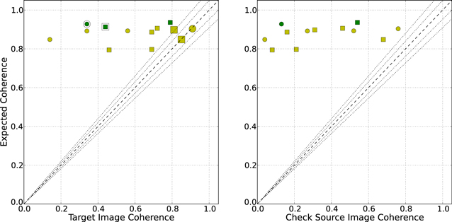
Figure 2. Comparisons of expected coherence as calculated from the phase rms plotted against the target source image coherence (left) and check source image coherence (right). Note that the phase rms used to calculate the expected coherence is measured from the bandpass source over the timescale equivalent to the phase-referencing cycle time, and hence acts as a proxy for phase residuals that would remain in the target after phase referencing. The circle and square symbols represent in-band and B2B modes, while the colors yellow and green represent band 9 and band 10 frequencies. In the left panel, the three larger symbols are for the observations where the phase calibrator and target are identical (i.e., 0° separation angle) whereas the outlined green circle and square indicate the band 10 observations that used the same setup with a target-to-phase-calibrator separation of 37. The dashed line is of equal coherence, and the dotted lines are ± 5% and ± 10%. From the stable phase conditions (Section 3.1.1) we expected at least >0.8 coherence for all images. Considering the left target source panel, only the three observations where the target and phase calibrator are identical match the expected coherence. All remaining observations have a finite target-to-phase-calibrator separation, and all have lower-than-expected coherence.
Download figure:
Standard image High-resolution imageAll but one of the five in-band observations have image coherence values <0.6, although >0.8 is expected. The only in-band observation to meet the expected value is EB X70fe, where the target and phase calibrator are identical (temporal referencing only, larger symbol). All but two of the eight B2B mode observations achieve an image coherence of >0.69, close to our pragmatic limit of 0.7. Of these, two EBs are where the target and phase calibrator are identical (larger symbols), while the other four observations use closer calibrators, <1°, when compared to the in-band observations. The remaining two B2B EBs with low coherence comprise the band 10 observation that purposefully used a more distant calibrator (Xf3ab—37) and X13757, which was observed down to very low elevation (see Appendix A.1).
In the right panel, we see that all check sources have an image coherence much lower than would be expected considering the phase rms. However, these check sources are farther away from the phase calibrator (22–65) when compared with the target sources per observation.
Table 5 reports the image parameters for the target sources, while Table 6 gives them for the check sources. The fitted flux is measured by fitting 2D Gaussian to the source, while the area flux is measured by integrating over a circular aperture with a 15 pixel radius centered on the source. In a number of cases, the larger area fluxes, when compared to the fitted fluxes, correspond to the spreading of source emission away from a pointlike structure as a result of calibration (phase) defects. For long-baseline observations, the aim is to resolve and correctly image small-scale structures around complex scientific targets, and hence it is imperative that the phase correction is accurate and that emission is not spread around the map (see also Section 3.4).
Table 5. Target Source Image Parameters from the HF-LBC-2019 Experiments
| Exec. Block | Target | Phase Referenced | Coherence | Peak/Flux | Self-calibrated | ||||||
|---|---|---|---|---|---|---|---|---|---|---|---|
| Suffix | Beam | Peak | Fitted Flux a | Area Flux b | Noise | Peak a | Fitted Flux a | Noise | |||
| (mas) | (mJy bm−1) | (mJy) | (mJy) | (mJy bm−1) | (mJy bm−1) | (mJy) | (mJy bm−1) | ||||
| In-band—Band 9 | |||||||||||
| Xb0b8 | J1259−2310 | 8 × 7 | 64.29 | 83.36 | 151.52 | 0.59 | 0.34 | 0.42 | 186.72 | 191.17 | 0.30 |
| X62b6 | J1259−2310 | 9 × 7 | 105.73 | 131.66 | 148.89 | 0.50 | 0.56 | 0.71 | 188.99 | 192.49 | 0.31 |
| X70fe c | J1713−3418 | 9 × 6 | 160.42 | 164.58 | 167.53 | 0.29 | 0.91 | 0.96 | 176.47 | 178.19 | 0.26 |
| X64c3 | J2229−0832 | 9 × 7 | 48.36 | 172.74 | 189.60 | 0.88 | 0.14 | 0.26 | 341.27 | 345.68 | 0.37 |
| In-band—Band 10 | |||||||||||
| X105d2 | J2229−0832 | 8 × 5 | 67.34 | 88.72 | 135.39 | 1.05 | 0.34 | 0.50 | 193.71 | 198.79 | 0.83 |
| B2B—Band 9-4 | |||||||||||
| Xda5c c | J1713−3418 | 9 × 8 | 151.18 | 149.10 | 144.71 | 0.49 | 0.85 | 1.04 | 177.53 | 178.12 | 0.31 |
| X13757 | J1259−2310 | 12 × 8 | 75.49 | 86.52 | 99.09 | 1.07 | 0.46 | 0.76 | 161.95 | 163.41 | 1.09 |
| X6945 | J1259−2310 | 12 × 7 | 127.90 | 133.49 | 139.71 | 0.61 | 0.69 | 0.92 | 185.37 | 182.68 | 0.50 |
| B2B—Band 9-6 | |||||||||||
| Xc5f1 | J1259−2310 | 10 × 8 | 118.52 | 119.09 | 122.74 | 0.52 | 0.69 | 0.97 | 171.73 | 168.99 | 0.35 |
| X7682 c | J1713−3418 | 14 × 7 | 139.62 | 144.80 | 151.13 | 0.53 | 0.81 | 0.92 | 171.71 | 174.60 | 0.45 |
| X5dcd | J2229−0832 | 7 × 7 | 242.64 | 245.91 | 236.42 | 0.78 | 0.72 | 1.03 | 337.69 | 324.54 | 0.44 |
| B2B—Band 10-3 | |||||||||||
| X7fe3 | J2229−0832 | 7 × 6 | 189.28 | 196.95 | 197.09 | 1.02 | 0.79 | 0.96 | 238.87 | 238.86 | 0.73 |
| B2B—Band 10-7 | |||||||||||
| Xf3ab | J2229−0832 | 7 × 5 | 108.56 | 114.73 | 183.40 | 1.22 | 0.44 | 0.59 | 246.31 | 244.91 | 0.78 |
Notes.
a Fitted flux from a 2D Gaussian fit to the central target source. b Integrated flux within a 15 pixel radius circle located at the center of the image—used for peak/flux ratio that is representative of how pointlike the image is, under the assumption that all of the flux is recovered within the circle. c Recall that the target source and phase calibrator are identical (0° separation angle, only temporal phase referencing). Beam reported to the nearest whole milliarcsecond.Download table as: ASCIITypeset image
Table 6. Check Source Image Parameters from the HF-LBC-2019 Experiments
| Exec. Block | Target | Phase Referenced | Coherence | Peak/Flux | Self-calibrated | ||||||
|---|---|---|---|---|---|---|---|---|---|---|---|
| Suffix | Beam | Peak | Fitted Flux a | Area Flux b | Noise | Peak | Flux | Noise | |||
| (mas) | (mJy bm−1) | (mJy) | (mJy) | (mJy bm−1) | (mJy bm−1) | (mJy) | (mJy bm−1) | ||||
| In-band—Band 9 | |||||||||||
| Xb0b8 | J1259−2310 | 8 × 7 | 40.79 | 54.41 | 113.89 | 0.94 | 0.27 | 0.36 | 152.82 | 165.12 | 0.67 |
| X62b6 | J1259−2310 | 9 × 7 | 78.42 | 103.38 | 115.58 | 0.86 | 0.52 | 0.68 | 152.03 | 154.76 | 0.72 |
| X70fe | J1713−3418 | 9 × 6 | 115.76 | 121.91 | 124.82 | 0.79 | 0.76 | 0.93 | 152.95 | 154.81 | 0.68 |
| X64c3 | J2229−0832 | 9 × 7 | 4.61 | ... c | 29.73 | 0.84 | 0.04 | 0.15 | 117.34 | 115.90 | 0.68 |
| In-band—Band 10 | |||||||||||
| X105d2 | J2229−0832 | 8 × 5 | 14.82 | 42.84 | 53.97 | 1.63 | 0.13 | 0.27 | 116.86 | 134.67 | 2.10 |
| B2B—Band 9-4 | |||||||||||
| Xda5c | J1713−3418 | 9 × 8 | 102.12 | 109.95 | 124.68 | 0.94 | 0.68 | 0.82 | 150.68 | 159.50 | 0.76 |
| X13757 | J1259−2310 | 12 × 8 | 45.18 | 213.39 | 199.17 | 4.40 | 0.08 | 0.23 | 568.78 | 598.96 | 2.47 |
| X6945 | J1259−2310 | 12 × 7 | 138.34 | 223.17 | 307.44 | 3.05 | 0.21 | 0.45 | 646.54 | 609.74 | 1.33 |
| B2B—Band 9-6 | |||||||||||
| Xc5f1 | J1259−2310 | 10 × 8 | 104.18 | 451.37 | 456.89 | 3.40 | 0.16 | 0.23 | 670.66 | 687.83 | 0.99 |
| X7682 | J1713−3418 | 14 × 7 | 50.12 | 66.77 | 75.78 | 1.24 | 0.31 | 0.66 | 161.60 | 162.19 | 1.07 |
| X5dcd | J2229−0832 | 7 × 7 | 85.15 | 97.23 | 121.71 | 0.94 | 0.46 | 0.70 | 186.57 | 175.11 | 0.65 |
| B2B—Band 10-3 | |||||||||||
| X7fe3 | J2229−0832 | 7 × 6 | 95.57 | 116.51 | 130.79 | 1.76 | 0.54 | 0.73 | 176.17 | 176.02 | 1.59 |
| B2B—Band 10-7 | |||||||||||
| Xf3ab | J2229−0832 | 7 × 5 | 38.78 | 54.24 | 76.92 | 1.81 | 0.29 | 0.50 | 132.25 | 135.17 | 1.60 |
Notes.
a Fitted flux from a 2D Gaussian fit to the central Check source. b Integrated flux within a 15 pixel radius circle located at the center of the source—used for peak/flux ratio that is representative of how pointlike the image is, under the assumption that all of the flux is recovered within the circle. c The fitting did not converge due to a poor image. Beam reported to the nearest whole milliarcsecond.Download table as: ASCIITypeset image
Based upon the metric of the phase rms, we expected high image coherence for all of our observations (>0.8). The fact that we do not see direct one-to-one correlations in expected and image coherence means that we need to carefully assess the degradation imparted due to the calibrator separation angle (Section 3.4), which is the only free parameter of these observations. Maud et al. (2020) expected a coherence loss of ∼0.2 for long-baseline observations made in band 7 (∼345 GHz) when using calibrators at ∼4° separation angle from the target source. In extrapolating their results to band 9 and 10, they reported that achieving >0.7 image coherence may not be possible. To address goal 1 outlined in Section 1, we report that even when the phase stability conditions are correct, and optimal, it is not a given fact that we will achieve the expected image coherence, and that a more careful consideration of the target-to-phase-calibrator separation angles is required.
3.2. B2B versus In-band
Figure 3 shows the pairs of in-band and B2B data sets that targeted the same source but did not necessarily use the same phase calibrators. The circles represent the observations taken immediately after one another on the same night, while the squares show those taken on different nights. Yellow and green colors again represent band 9 and band 10 data, respectively, while the larger symbols highlight the observations where the target and phase calibrator are identical, and the circled symbol highlights the band 10 experiments using the phase calibrator 37 from the target.
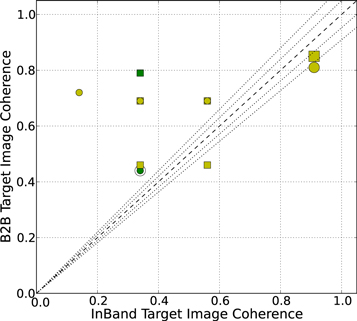
Figure 3. Comparisons of the in-band and B2B mode target image coherence that observe the same source. The circle and square symbols represent paired and unpaired observations, in that paired observation are taken on the same night in each mode, while unpaired match observations are taken on different nights. The colors yellow and green represent band 9 and band 10 frequencies. The two larger symbols highlight the observation pairs where the phase calibrator and target were the same source (i.e., 0° separation angle) whereas the outlined green circle indicates the paired band 10 observations that used the same target and phase calibrator with a 37 separation angle. The dashed line is of equal coherence, while the dotted lines are ± 5% and ± 10%. Except those using the same calibrators, the B2B used closer calibrators compared to the in-band mode and typically achieved a higher coherence.
Download figure:
Standard image High-resolution imageThe B2B data sets typically have a higher image coherence. Except the unique data sets mentioned above, all in-band observations use phase calibrators farther from the target source than the paired B2B observations (e.g., Maud et al. 2020). We note that the B2B EB X13757 has much lower-than-expected coherence, which is due to the low source elevation during the latter half of the experiment (see Appendix A.1).
For the experiments where the phase calibrator and target are identical (larger symbols), the image coherence is high, and the in-band and B2B values are within a 0.1 of each other. This supports the findings of Maud et al. (2020, 2022), who reported that the in-band image coherence will be marginally higher than the B2B image coherence, as the DGC step can cause a slight degradation for the B2B mode.
In our band 10 experiments that use the phase calibrator at 37 (in-band X105d2 and B2B Xf3ab, circled symbol) the B2B image coherence is slightly higher, but still within 0.1 of the in-band value. Despite selecting optimal calibrators, we did use SPW combination to achieve a sufficient S/N for the in-band data, while flagging of each data set was also slightly different. Hence, we do not over-interpret this as evidence that B2B is superior at Band 10, simply that the data reduction can cause slight, few percent, differences.
Figure 4 shows the target source images from six observations and compares the in-band (left) and B2B (right) calibration modes. In all cases except where the target and phase calibrator are identical (top—X70fe and Xda5c), the B2B data used a closer calibrator and indicate a higher image coherence and more pointlike image structure.

Figure 4. Target images for a selection of in-band (left) and B2B (right) observations. The top panels show the band 9 EBs X70fe and Xda5c where the target and phase calibrator are identical (i.e., 00) and make up an ideal scenario; the middle row shows band 9 EBs Xb0b8 and Xc5f1 using 38 and 08 separated calibrators; the bottom plots show the band 10 EBs X105d2 and X7fe3 using 37 and 07 separated calibrators. Each pair of plots uses the same color scaling. Contours are drawn at −5σ (black dotted), 5σ, 15σ, 25σ, and 50σ (color), where σ are listed in Table 5. Note that, except for X70fe and Xda5c, the right panel B2B observations have higher image coherence and more pointlike image structure; strong central emission is colored black. The beams are shown at the bottom left of each panel.
Download figure:
Standard image High-resolution imageIn addressing goal 2 as outlined in Section 1, when comparing in-band and B2B modes, we advocate that in stable atmospheric conditions any observation using a phase calibrator at a given distance from a target source will provide target images of equal quality regardless of the mode used, in-band or B2B. It is apparent that the observations using the closest phase calibrators will always provide the most optimal phase correction, and the closer calibrators will be provided by the B2B mode.
3.3. Quality of Phase Correction
In order to understand the quality of the phase calibration, other than as measured from image parameters, we examine the average phase offset and phase rms, per antenna, of the target sources after phase referencing. These parameters from a subset of six observations are shown in Figure 5. The left panels are in-band observations while the right panels are the paired B2B observations of the same target source. The gain tables from which the values are extracted were produced from the self-calibration solutions using the scan time for the target sources after phase referencing. For plotting clarity, we extract only the solutions of all antennas with the reference antenna, although all baselines follow the same trend. Ideally, after phase calibration the targets should be point sources at the pointing center such that the gain solutions should have a zero degree average phase offset and where the phase rms was reduced down to the expected level when considering the atmospheric variations (Section 3.1.1). In each plot the upper section indicates the phase rms while the lower section shows the phase offset, both as a function of baseline length from the reference antenna. The gray bars show the median values, while the dotted gray line for the phase offset is the standard deviation when considering the averages of each antenna. The dashed black lines are the expected values that (for the phase rms) are taken from Table 1, while for the phase offset, the expected value is 0°. Antenna-averaged phase offsets and residual phase rms values from all experiments are listed in Table 7.

Figure 5. Phase rms and phase offset as a function of baseline length for all antennas with the reference antenna for a selection of in-band (left) and B2B (right) observations extracted from scan-based solutions (note that all baselines follow the same trend but are not shown for clarity). The top of each plot shows the phase rms while the lower part shows the phase offset. The red points indicate the data while the gray bars show the median values. In the lower sections, the dotted gray lines are the standard deviation of the offset averages accounting for all antennas. The dashed black lines are the expected values, for phase rms from Table 1; for the offset it is zero degrees. The top panels are for EBs X70fe and Xda5c, and depict an ideal scenario, as the phase calibrator and target are identical. The middle and bottom panels show representative band 9 and band 10 cases, respectively. Overall the in-band uses a more distant calibrator that does not reduce the phase rms down to the expected level. For the B2B observations using closer calibrators, the phase rms is reduced by over a factor of 2 compared to the in-band data.
Download figure:
Standard image High-resolution imageTable 7. Residual Phase rms and Phase Offset of the Observed Target Sources
| EB | Phase rms (deg) | Phase Offset (deg) |
|---|---|---|
| In-band—Band 9 | ||
| Xb0b8 | 85.5 | −5.0 ± 12.8 |
| X62b6 | 52.6 | 3.4 ± 21.9 |
| X70fe a | 22.1 | −3.3 ± 1.9 |
| X64c3 | 87.4 | 7.9 ± 12.8 |
| In-band—Band 10 | ||
| X105d2 | 81.1 | −37.2 ± 12.2 |
| B2B—Band 9-4 | ||
| Xda5c a | 23.4 | 5.5 ± 9.9 |
| X13757 | 57.0 | −16.8 ± 20.2 |
| X6945 | 36.4 | 22.6 ± 16.0 |
| B2B—Band 9-6 | ||
| Xc5f1 | 46.4 | −2.5 ± 10.1 |
| X7682 a | 25.7 | 2.8 ± 10.4 |
| X5dcd | 33.3 | −17.0 ± 16.6 |
| B2B—Band 10-3 | ||
| X7fe3 | 36.3 | −29.1 ± 14.1 |
| B2B—Band 10-7 | ||
| Xf3ab | 70.9 | −8.9 ± 14.8 |
Note.
a The target and phase calibrator are identical.Download table as: ASCIITypeset image
The ideal case is illustrated by the in-band EB X70fe and the B2B EB Xda5c in the top panels of Figure 5 where the target and phase calibrator are identical. Both plots show a near 0° phase offset and a median phase rms slightly better than expected. We acknowledge that the apparent improved phase rms in these cases is likely due to the fact we use scan-based solutions rather than the integration time (as due to S/N requirements). Thus, we likely miss some of the real (i.e., not S/N related) short-term, seconds-long timescale variability. The B2B mode has a larger scatter in the phase offset values that is likely imparted from the DGC step (also see Maud et al. 2020). The phase offset scatter is also larger in the B2B EB X7682, which is not shown but where the target and phase calibrator were also identical.
For the band 9 data, we show the in-band observation Xb0b8 and the B2B observations Xc5f1 in the middle panels of Figure 5. These both have phase offsets with an average close to zero degrees with a similar spread. However, the phase rms is almost 90° for the in-band observations, significantly higher than the expected ∼27°, while it is ∼46° for the B2B observation. The B2B data do not achieve the expected value of ∼28°, but the phase rms is over a factor of 2 better than the paired in-band observation. Given the finite calibrator-to-target separation, it is not unreasonable to consider that the larger difference in sky position from the target to phase calibrator hinders the phase-referencing effectiveness. Regardless of using the scan-based solutions, the phase rms in these cases is likely dominated by the suboptimal calibration creating considerable scatter rather than any underlying small timescale variability. Note that the B2B observation may also have a higher-than-expected phase rms because the source elevation in the latter half of the observation is low (<40°), such that the expected phase rms is likely underestimated when scaled from the bandpass scan in comparison to the median target elevation. The two-lowest elevation B2B observations X13757 and X6945 (not shown) both have average phase offsets of ±20°, which could also be a consequence of the low elevation impacting the DGC solutions.
At band 10 we compare the in-band EB X105d2 and the B2B mode using a closer calibrator in EB X7fe3 in the bottom panels of Figure 5. Both have a similar average offset with a similar spread. Most noticeable is that the in-band phase rms is >70° after phase referencing and points to a coherence loss of ∼0.5. By comparison, the B2B observation phase rms is less than half the in-band value (∼36°), although it is not quite as low as expected (∼21°). The target source elevation is >45° during this observation, and thus the higher-than-expected phase rms can only be attributed to the finite separation of the target and phase calibrator, despite it being <1°. The coherence calculated from the phase rms remaining in the target data after B2B phase referencing is 0.81 and is comparable with the image coherence achieved of 0.79. We note that the band 10 B2B EB Xf3ab (not shown) that uses the same calibrator setup as X105d2 (separation from target of 37) also has a similarly poor phase rms (∼70°). This suggests such a separation angle is already too distant to provide any useful reduction in phase rms when employing phase referencing for band 10 long-baseline observations. The phase offset for Xf3ab is also nonzero, but is ∼20° better than X105d2. Nonzero phase offsets for the in-band observations could point to underlying antenna position uncertainties and cannot be excused as caused by the DGC step as for B2B data. That said, DV01 was used for the reference antenna in all data, and the phase offsets do not appear to be biased across the different observations. We acknowledge the fact that at the highest frequencies the antenna position uncertainties will be more acute and hence act to create more defects in the image. We can only state that careful and accurate measurements of the antenna positions are important when conducting such high-frequency observations.
To address goal 3 outlined in Section 1, we find that only the observation with closest calibrators, those using B2B mode in this case (excluding our experiments where the target and phase calibrator are identical), can provide a reduction in phase rms to almost the expected level. When the phase calibrators are too distant, as has been shown before by Asaki et al. (2016) and Maud et al. (2020, 2022), phase referencing is ineffective at notably reducing the phase rms and combating decoherence. The phase offsets averaged over all antennas are generally within 10° of zero for all of our observations, supporting that the phase referencing accurately positions the source, on average, to the pointing center during imaging.
3.4. Image Parameters with Separation Angle
Figure 6 shows the image coherence of both the target and check sources as a function of the target-to-phase-calibrator (and check-to-phase-calibrator) separation angle. Yellow and green represent band 9 and 10 observations, while the circles and squares indicate in-band and B2B modes, respectively. The smaller symbols are those for the check sources. The lower limit bars illustrate the coherence we might expect if we had compared with the integration self-calibrated images (we increased the self-calibrated image peak flux to account for the expected reduction when considering the phase rms). The observation where the target and phase calibrator are identical provides an anchor point at 0.0° (X70fe, Xda5c, X7682). For these observations, we see a loss of coherence from only the temporal phase-referencing process before we even considering moving to a different sky location. For these three data sets, we see that the in-band experiment has the best image coherence and corresponds to that expected when calculated from the phase rms (see Table 1). The two B2B observations are slightly worse, and we attribute the extra image coherence reduction to the DGC step (see also Maud et al. 2020). When moving to larger separation angles, it is clear that the image coherence degrades rapidly. Within the parameter space of these experiments, the degradation in image coherence can be approximated to a linear fit (intercept = 0.8, slope =−0.109 ± 0.014). We do not separate the band 9 and 10 data, nor the in-band or B2B modes given the low number statistics.

Figure 6. Target and check source image coherence as a function of separation angle to the phase calibrator. As in Figure 2, the circle and square symbols represent in-band and B2B modes, while the colors yellow and green represent band 9 and band 10 frequencies. The smaller symbols are for the check sources, the larger for the targets. The lower limits are the coherence values calculated when scaling up the self-calibrated image peak fluxes to account for any flux loss due to phase rms (see Section 3.4). The dashed black lines are the linear fits to all data points. The degradation of coherence follows the same slopes within the fit uncertainty, although the intercept for the coherence is 0.8 at 00 separation angle. The black solid line show values from corruption models that add antenna position uncertainties, yellow from a variable phase screen, and green using both antenna positions uncertainties and the screen model (the dashed and solid lines represent parallel and perpendicular phase-referencing direction offsets with respect to the phase screen motion—see Section 4).
Download figure:
Standard image High-resolution imageTo address goal 4 outlined above, considering that all of our observations were taken in stable atmospheric conditions (Section 3.1.1), we can already quantify that with a coherence requirement of >0.7 (Asaki et al. 2020a, 2020b; Maud et al. 2020), 16 km baseline high-frequency observations (>660 GHz) with ALMA need to use phase calibrators within ∼1°. Compared with the extrapolated results from Maud et al. (2020), who predicted band 9 observations up to maximal baselines of 8.5 km require a 1° separation angle, we find that reality is more optimistic. If a reduced image coherence is acceptable when considering the operational difficulties of such high-frequency long-baseline observations (see Section 4.4), then image coherence levels of ∼0.6 and ∼0.5 are expected for separation angles at ∼2° and ∼3°, respectively. Further investigation on separation angle effects are detailed in Section 4.
3.5. Flux Continuity
The absolute flux accuracy of ALMA at the higher-frequency bands is quoted as 20% in the documentation 14 . Considering the fluxes after self-calibration, regardless of the initial observing mode, at band 9: J1259−2310 ranges from 163.41−192.49 mJy, J1713−3418 from 174.60−178.19 mJy, and J2229−0832 from 324.54−345.68 mJy, while at band 10 the only target J2229−0832 ranges from 198.79−244.91 mJy. The percentage differences when considering these minimum and maximum values are 16.0% for J1259−2310, 2% for J1713−3418, and 6% for J2229−0832 at band 9, which are all within the accuracy reported by ALMA. The difference is 21% for J2229−0832 at band 10. We did ensure the use of the same calibrators for the amplitude scaling, but note that the fluxes extracted from the ALMA catalog did vary depending on observing date. It is also important to note that our self-calibration process used the scan time for these targets, not the integration time where the S/N was significantly reduced, and hence the fluxes of the targets after self-calibration should be regarded as lower limits. We do see some minor residual extended flux in the band 10 image of J2229−0832 from the in-band observation X105d2, which, if accounted for, boosts the flux to ∼220 mJy and thus would be within ALMA's prescribed uncertainty. Using the estimated phase rms and scaling between the integration and the scan times for the target sources, we expect an 8% flux reduction on average compared to ideal integration time self-calibration, which could be considered as an added uncertainty in our fluxes.
We cannot comment on longer-term high-frequency flux accuracy greater than a few days, but in reality for a given ALMA array configuration and such high frequencies, any user observations would likely be completed within a short period of time while all observing parameters are suitable. Of course, a main caveat is that not all targets can be self-calibrated, and thus it is absolutely imperative that ALMA users fully understand the effects of decoherence for these challenging observations, as the target source flux without self-calibration can be >20% discrepant regardless of the absolute flux accuracy adhering to the ALMA quoted uncertainties. Only in the observations where the target and phase calibrator were identical did we achieve a target coherence >0.8, while even using close calibrators in the B2B mode and with good phase stability conditions all target sources lost more than 20% of the peak flux density.
4. Analysis
In this section we investigate the trends in decreasing image coherence with separation angle when corrupting data ideal with phase errors. In this case we self-calibrate the target, J2229−0832, from EB X64c3 using the integration time, which was possible for J2229−0832, as it is the brightest target in our experiments with a peak flux of 397.94 mJy bm−1 (after integration (2 s) based self-calibration, note that this is ∼14% more than the scan-based self-calibration, roughly as expected for this EB with a phase rms of 329 over 59 s). We corrupt this data building from the simple model shown in Maud et al. (2020) accounting for antenna position uncertainties and then add further corruptions using a simplified model atmospheric phase screen that follows the frozen-screen approximation built following the prescription in the ARIS code (Asaki et al. 2007)
15
. Further details of the phase screen model are provided in the Appendix.
4.1. Degradation Cause by Antenna Position Uncertainty
We follow exactly the procedure outlined in Maud et al. (2020) in using the trend in antenna position uncertainties as measured by Hunter et al. (2016) to calculate phase corruptions. For completeness, as per Maud et al. (2020), the path length uncertainties ℓ(μm) are calculated as Δρ · Δθ where Δρ is the baseline position uncertainty and Δθ is the calibrator-to-target separation angle (in radians). As a function of baseline length, b, the uncertainties are: east (0.140 mm + b km · 0.071 mm km−1); north (0.110 mm + b km · 0.054 mm km−1); and vertical (0.220 mm + b km · 0.198 mm km−1). A value is randomly attributed to each antenna, as separated from the reference antenna, from a Gaussian distribution centered on the absolute uncertainty with standard deviations in the east, north, and vertical directions of 0.086, 0.076, and 0.129 mm and 0.121, 0.118, and 0.296 mm for baselines shorter and longer than 2.5 km, respectively. Corrupting gain tables are created using gencal in casa for calibrator separation angles ranging from 1.0−70 (in 10 steps). The errors manifest as almost constant phase offsets per antenna.
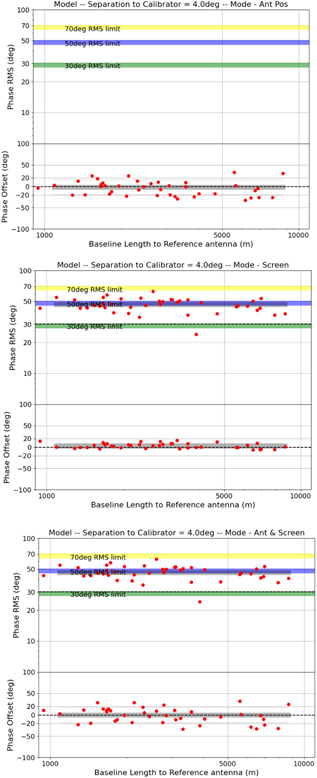
The top panel in Figure 7 shows the residual phase rms and phase offset remaining for the target source after corrupting the ideal target data with the antenna position uncertainties assuming a phase-calibrator-to-target separation angle of 40. As there was no phase noise added, the phase rms is 0°; however, the phase offsets can reach > ± 20° for some antennas. The average offset considering all antennas still remains close to 0°. In contrast, the largest angular separation case observed (38; bottom panel in Figure 5) has an overall phase offset and suggests there is a more systematic antenna position uncertainty for those observations. We surmise that it is possible for the antenna position uncertainties to be more systematic across the array in contrast to random values for our corruption process.
Figure 7. Plots of phase rms and phase offset as a function of baseline length to the reference antenna for the target source as corrupted by antenna position uncertainties (top), frozen-flow screen phase referencing (middle), antenna position uncertainties, and screen phase referencing (bottom). In the top panel, the phase rms is not plotted as this is exactly 0°, and antenna positions uncertainties only corrupt the phase offset. The lines are as per Figure 5, and in each panel, the upper and lower sections show the phase rms and phase offset. The screen model alone (middle) dominates in corrupting the phase rms, which is ∼50° after phase referencing despite the phase rms conditions of the model being set at 30° as measured over 60 s for a single source. There is little change in the phase offsets. The bottom plot combines both antenna positions and the screen model corruptions.
Download figure:
Standard image High-resolution image
The solid black lines in Figure 6 indicate the reduction in image coherence with separation angle. As Maud et al. (2020) also found, the antenna position uncertainties alone cannot explain the degradation of the target images, and in fact the image coherence does not begin to fall below 0.9 and 0.8 until separations angles of ∼4° and ∼6°, respectively.
4.2. Degradation due to the Sky Position
Maud et al. (2020) extensively discussed the unaccounted for degradation of their target images as caused by suboptimal phase referencing. In Figure 5 we also identified that even after phase referencing the target residual phase rms can be significantly higher than the expected phase rms. Simply, calibrating a target using solutions from a vastly different patch of sky is unlikely to provide a reasonable phase correction. To examine the effect more closely, we use a frozen-flow turbulent phase screen model (see the Appendix) to create mock observations using calibrators separated from the target by 00–70 (in 10 steps). The 00 case is that where the target and phase calibrator are identical and only temporal phase referencing occurs.
In short, each antenna is assigned absolute path length values from the screen (i.e., a phase value) for the target and phase calibrator as a function of time and position. The screen is moved at a representative speed of 5.0 ms−1 (Table 1), while a position offset is also included for the phase calibrator scans as a function of separation angle from the target. The direction of the position offset can be parallel or perpendicular to the screen motion. The phase rms level is normalized to 30° over a 60 s period when observing a single source through the phase screen as to match the conditions of our experiments. The model phase screen corruptions for the target and phase calibrator are applied to the self-calibrated (ideal) data and essentially create mock raw observational data. Phase calibration is then undertaken, as would be conducted for real observations, and phase transfer is made to the target before imaging. Further details are provided in the Appendix.
In Figure 6 the yellow lines indicate the image coherence after phase referencing through a mock phase screen as a function of separation angle (dashed and solid lines represent position offsets for the phase calibrator parallel and perpendicular to the screen motion, respectively). For consistency with our observations, we calculate the image coherence compared with the scan time self-calibrated image of J2229−0832 that has a flux of 345.68 mJy bm−1 at band 9 (EB X64c3, which is lower than the integrated self-calibrated value; see above). At 00 the image coherence is 0.8, as expected given the remaining phase rms over the cycle time. However, as a function of increasing separation angle, the image coherence degradation from the phase screen model is not as extreme as the observations themselves. At worst, the coherence is ∼0.6 at 7° in the case where the phase calibrator offset position is perpendicular to the screen motion. We understand that the worse image coherence, in this case, is caused by the lack of any possibility to align the target phase variations with those of the phase calibrator. For a given baseline, such a case may occur when the phase calibrator position offset direction through the screen is parallel to the screen motion because the target will see the same phase variations as the phase calibrator when they arrive some time later due to the screen motion (e.g., Asaki et al. 1998).
In the middle panel of Figure 7 the residual phase rms and phase offset remaining for the target source after corruption from the phase screen model using phase referencing with a 40 calibrator is shown. The phase rms remaining even after phase referencing is ∼50° despite the phase rms conditions setting the model at 30°. It is clear that the different lines of sight through the model screen mean that the target is not optimally calibrated, although the remaining phase rms is notably lower than in our observations (Figure 5). There is also little change in the phase offsets indicating that the screen model acts only to spread the phase offset due to underlying uncorrected long-term phase variations between the target source and phase calibrator. We do not see systematic offsets, as is also apparent in the observational data (Figure 5), suggesting that the change in phase at the positions of the target and calibrator is not significantly different.
The phase screen model itself is not the focus of this paper; however, it is worth noting caveats due to our simplifications and possible modifications for the future. The phase screen is a single-layer static frozen flow where it simply moves over the array with fixed Kolmogorov turbulent power scales (Dravskikh & Finkelstein 1979), where the line of sight of each antenna is through a single pixel in the screen, and where we assume the screen height and wind speed are representative. For certain baselines, considering the time between the target and calibrator scans and the screen motion, the target will be well corrected as the frozen in-phase variations match up for the calibrator as they were recorded for the target (see Asaki et al. 1998). In reality, a finite thickness phase screen with constant variability in all directions along with a general screen motion would likely be a more realistic representation. The turbulent power scaling is only one representation of the variations and does not always necessarily match those at the ALMA site, which do vary (Matsushita et al. 2017). We also model an idealized case of a zenith observation without any additional scaling for a different line-of-sight path between the calibrator and target source, and so we expect that elevation scaling would become more important for larger separation angles and low elevation <40°–50°. Most notably, the phase differences between the target and phase calibrator are insufficient in corrupting the model target. An increase in screen speed and/or the turbulent layer height would increase the distance, on the screen, for the lines of sight to the target and calibrator and should result in a worse calibration of the target. Ishizaki & Sakamoto (2005) used two short (300 m) test baselines at the ALMA site to measure the screen speed. Their best fit indicates that the screen speed is 1.2 times greater than a ground-based wind measurement, and as such, the small increase for our screen model is unlikely to cause sufficient additional corruption. Ishizaki & Sakamoto (2005) also reported that the screen height should generally be <1000 m, counter to what we require in the models. One possibility, as introduced by Asaki et al. (2016) to explain a notable worsening of the phase rms on the long baselines (as compared to short baselines) of their targets after phase referencing with distant calibrators, is that a second high-altitude layer (∼15–20 km) with less turbulence but a faster screen speed could provide an additional phase difference between a target and phase calibrator. We recommend a detailed parameter space investigation of such screen models for future studies.
4.3. Combined Phase Corruption
The final case to examine is that of both the phase screen and antenna position uncertainties. The green lines in Figure 6 indicate the image coherence as caused by phase corruptions from the screen models with parallel (dashed) and perpendicular (solid) phase calibrator offsets applied in concert with the corruption in antenna positions.
For both cases with parallel and perpendicular phase calibrator position offsets, the coherence losses appear dominated by the antenna position uncertainties. Only beyond a ∼3° separation angle do we see additional coherence loss compared to what the antenna uncertainties cause alone. The perpendicular case provides a further 2%–3% coherence loss. However, neither case provides enough degradation for the image coherence to match that seen in the experiments. The overall coherence loss is not simply the sum of the corruptions caused by the antenna position uncertainties and phase screen applied alone. The bottom plot in Figure 7 shows the residual phase rms and phase offsets remaining for the target source. Comparing with the top and middle panels, we see that the bottom panel is the combination of the antenna positions dominating the phase offset, with the phase rms provided by the phase screen model. However, in comparing with the observations presented in Figure 5 for the 38 separated calibrator, we can see that the residual phase rms is lower from our models, i.e., there is not enough phase rms corruption.
In light of the above discussion, with a detailed screen model investigation, we would expect that the combined effect of the screen and antenna positions would be broadly representative of the experiments overall. Here we summarize that both components, sky position between the target and calibrator and antenna position uncertainties, must be acknowledged for high-frequency long-baseline observations despite the fact that the phase rms as parameterized by a measurement of a strong source would have suggested very stable conditions (phase rms ∼30°). At present, our current corruption models are too optimistic.
4.4. Calibrator Availability
Using the Phase rms Database (Maud et al. 2023), we take all unique target sources stored (6757) and compare each with the calibrators from the ALMA calibrator catalog 16 in a target–calibrator pair matching exercise. We use a best-case scenario to calculate the required calibrator fluxes, assuming bandwidths of 15.0 and 7.5 GHz for in-band and B2B modes, respectively, 12 s scan times, and an S/N requirement of 15. For B2B we use an S/N of 45 as the scaling of the calibrator solutions also scales the noise (we use a factor of 3 for ease, but this should strictly be the ratio of the high-frequency to the low-frequency band pair). At Bands 9 and 10, we would need calibrators of 247 mJy and 638 mJy, and at band 3, 4, 6, and 7 (for the B2B modes related to bands 9 and 10 used in this work) calibrators would need to be 34, 36, 45, and 66 mJy, respectively. Table 8 shows the median separation angles and also the percentage chance that a calibrator is within 1°, 2°, and 3° (see also Asaki et al. 2020a). We highlight the effectively zero chance for finding in-band calibrators, while B2B, although still difficult, will allow a good portion of observations to be conducted.
Table 8. Parameters for In-band and B2B Phase Calibrators
| Calibrator | Required | Median | Chance (%) within | ||
|---|---|---|---|---|---|
| Band | Flux Density | Separation | 1° | 2° | 3° |
| (mJy) | Angle (deg) | ||||
| In-Band | |||||
| 9 | 247 | 7.5 | 2.4 | 6.4 | 12.0 |
| 10 | 638 | 18.5 | 0.5 | 0.8 | 1.6 |
| B2B | |||||
| 3 | 34 | 1.8 | 22.9 | 61.6 | 86.6 |
| 4 | 36 | 2.0 | 19.4 | 50.0 | 79.9 |
| 6 | 45 | 2.2 | 17.0 | 44.9 | 74.8 |
| 7 | 66 | 2.4 | 14.4 | 40.2 | 66.0 |
Notes. The S/N is 45 considering the flux densities for the B2B mode.
Download table as: ASCIITypeset image
4.5. Recommendations for High-frequency ALMA Observing
In the short (immediate) term, we recommend that the empirical trend from the limited data we have available is the best parameterization of expected image corruption when observing in the correct conditions for PI observations. We follow the same recommendations as Maud et al. (2020) suggested from their lower-frequency data, and state that the phase rms stability should be <30° over the intended phase-referencing cycle time while the phase calibrator should be within the strict limit of 1° if we are to expect a target image coherence >0.7 for bands 9 and 10, after phase referencing (and standard WVR corrections). This should ensure that any high-frequency observation, irrespective of the target source strength, can be calibrated to a sufficiently high quality. As we have illustrated, in operations the use of the so-called go/no-go stability checks are suitable, and should continue to be used, for measuring the stability. We caution that with our limited number of test observations we do not separate in-band and B2B data and cannot comment directly on the minor negative effect the DGC step imparts. For consideration, we can assume that the fast frequency switching employed at bands 9 and 10 for the DGC scans would yield a phase rms residual <20°–25°, and when following the parameterization in Maud et al. (2020), a 0.05 difference in image coherence between in-band and B2B observations is likely.
We highlight that self-calibration can also be considered for the brightest targets, but caution that it should not be depended on a priori. ALMA undertakes quality assurance (see Petry et al. 2020) as to confirm the user requirements are met, and in some cases observations are re-queued if these are not. For high-frequency long baselines, the calibrator separation angle could be relaxed (>2°–3°) if self-calibration was guaranteed, such that the target source properties drive the final phase correction accuracy. However, if after the observation self-calibration was not possible, due to unknown changes in the target source, then the final products would be degraded or in the worst case useless due to using too distant calibrators. Indeed, a high priority for ALMA in 2023 is to include self-calibration into pipeline calibration (Hunter et al. 2023 submitted) as to achieve the most optimal products if it can be conducted. Considering the flux requirements outlined in Table 8 for pointlike calibrators, science targets at bands 9 and 10 do need to be sufficiently bright, and likely more than shown in Table 8 if they are extended (see also, Asaki et al. 2023 submitted) and dependent on the solution S/N and the self-calibration timescale. Although it is easier to find more distant calibrators, we reaffirm that the strict criteria above (i.e., ∼1° calibrator-to-target separation angle) must be adhered to, in particular for weaker targets where self-calibration is not possible.
In the long term, it may be worth considering whether a more realistic phase screen model could be built at runtime from measurable observing conditions and used to dynamically adjust the observing scenario. Maud et al. (2022) outlined how the phase rms measured as a function of time can be used to adjust the observing cycle time to meet a given requirement, i.e., using faster phase referencing to reduce the phase rms (see also Holdaway 2001) or slower referencing in stable conditions as to improve efficiency. If, in aligning measurable parameters from, for example, a bandpass-like scan, one could build a more realistic phase screen model, it could be used to assess whether with the suggested cycle times were feasible in achieving a give coherence level for the available calibrators or if another observation would be better suited to the conditions. A phase-referencing experiment could also be conducted before observations take place, similar to the go/no-go test. However, it is likely to be time consuming in requiring numerous visits to two or more QSOs on the sky in order to reasonably establish the image coherence after conducting phase referencing. Investigations into improvement of antenna position measurements may also alleviate the strict limitation on the calibrator-to-target separation angle, which could be tested in future long-baseline campaigns, while elaborate paired antenna calibration scenarios could also be envisaged.
5. Summary
We conducted 13 experiments at bands 9 and 10 using both in-band (5) and B2B (8) observing modes as part of the ALMA high-frequency long-baseline campaign in 2019 (HF-LBC-2019) to investigate the feasibility of calibration and imaging for the most extreme observations that ALMA can make. Checks of the phase stability using standalone go/no-go stare observations were accurate in predicting the phase rms before the experiments were undertaken as was confirmed by measuring the phase rms stability directly from the bandpass sources within the experiments themselves. All observations were made in conditions where the phase rms was <40° over the phase-referencing cycle time, which corresponds to an expected image coherence of >0.8 after calibration and under the assumption of perfect phase referencing. All observations could be calibrated and imaged but the results varied in quality and did not necessarily achieve the expected coherence based only on the phase stability.
In comparing realistic scenarios where in-band observations use slightly more distant calibrators (37–38) compared to paired B2B observations with close calibrators (0.7-08), we find that the B2B mode, despite any extra uncertainties imparted through the DGC step, produces a better calibration in terms of reducing the target source phase rms and in yielding higher image coherence. The difference is solely driven by the calibrator separation angle difference. Irrespective of observing mode, all experiments using a finite target-to-phase-calibrator separation angle do not fully reduce the phase rms down to the expected level, as measured from the phase stability. Only in three experiments, one in-band and two B2B EBs, where the target and the phase calibrator were identical (00 separation angle) such that only temporal phase referencing occurred, did the image coherence correspond within 0.1 of the expected value. In all other cases, the resultant image coherence was lower than expected. The degradation of image coherence is found to be a function of the target-to-phase-calibrator separation angle, following a slope of −0.109.
Models that corrupt the phases of a target source due to phase referencing within a simplistic frozen-flow atmospheric phase screen while also accounting for typical antenna position offsets currently provide an overly optimistic scenario when compared with the image coherence degradation observed. Our phase screen model needs to add further realism in order to better replicate the empirical findings.
After self-calibration of the target sources, we report that the flux continuity is generally within the 20% absolute flux uncertainty limit set by ALMA provided that the same flux calibrator is used across the different observations. That said, the community should be clearly notified of the, potentially, significant reduction of image coherence and loss of flux in their target images that exceeds 20% after normal phase referencing for such difficult high-frequency long-baseline observations. Importantly, the reductions in peak flux density and integrated flux of any science target due to inaccuracies from phase referencing should not be confused with the reported absolute flux calibration uncertainty and must be considered as an additional source of error during scientific interpretation.
Our investigations support that the process for selecting the optimal calibrator mode based on calibrator availability and separation angle degradation (Maud et al. 2020) still holds for ALMA long-baseline observations using band 9 and 10. Positively, we confirm that ALMA high-frequency long-baseline observations are feasible in delivering high-quality target images using phase referencing provided that strict limits are adhered to. Any future ALMA high-frequency long-baseline (16 km) observations should be conducted in stable atmospheric conditions where the phase rms is <30° as measured over the phase-referencing cycle time, and a phase calibrator separated by ∼10 from the target at bands 9 and 10 must be used if the target image coherence after phase referencing is to be >0.7. If worse image coherence is acceptable and image structure defects are understood, or for example if target sources can later be self-calibrated, more distant calibrators out to ∼20 or ∼30 can be used, in which case the image coherence is expected to be ∼0.6 and ∼0.5, respectively, after phase referencing.
Acknowledgments
ALMA is a partnership of ESO (representing its member states), NSF (USA) and NINS (Japan), together with NRC (Canada) and NSC and ASIAA (Taiwan), and KASI (Republic of Korea), in cooperation with the Republic of Chile. The Joint ALMA Observatory is operated by ESO, AUI/NRAO, and NAOJ. We would also like to thank all of the Joint ALMA Observatory staff in Chile for performing the challenging HF-LBC-2019 observations successfully, and extend specific thanks to Eric Villard for his valuable expertise. Furthermore, we extend a deep gratitude to all technical and engineering staff without whom these observations would not have taken place, along with gratitude to all that have worked previously on the B2B mode, and are too many to name. L.T.M. and T.T. were adopted as JAO ALMA visitors during their stay at JAO during the campaign. Finally, and absolutely not least, we would like to dedicate this publication to the late Richard Hills, who, in some way, shape, or form has been interwound with many of us throughout our journey and careers at ALMA; he will be sorely missed.
Appendix: Phase Screen Model Process
A phase screen is built using ARIS following a typical Kolmogorov turbulence as described in Asaki et al. (2007) and is shown in Figure 8 (see also, e.g., Martí-Vidal et al. 2010). In generating the screen, the change between inner and outer scale, or 3D to 2D turbulence where the power law becomes shallower for larger scales, is set to 1000 m. The individual pixels correspond to a 10 m size resolution element while the screen is 8192 × 2048 in size and hence is large enough to cover the long-baseline array configuration as well as extending enough such that we can propagate the screen over the array in order to replicate a frozen-flow turbulent layer. In building the screen, the farthest corners of the model screen are set with a variable seed and all other variations then propagate inwards as variations from these.
In order to create mock phase-referencing observations, an initial calibration gain table is built for the target and phase calibrator using gaincal in casa to produce integration time (∼2 s for these data) solutions, which are to be overwritten. During this process, the minimal required S/N input in gaincal is set to 0.01. As the values of the solutions are not important, this step is only to create a correctly structured gain table. From the phase screen, we attribute phase components to the target and the phase calibrator for each integration by association with corresponding antenna positions while moving the screen at an assumed wind speed. During integrations where there are no data recorded for the target or the phase calibrator, such as the slew time or where system temperature measurement occurred, the screen is still propagated. We also build baseline-based phases by storing ∼15 minutes of continual antenna-based phases and use them to assess the SSF and establish a scaling factor to set the desired maximal phase rms level. To closely match the typical conditions of our experiments, we scale the model phase variations input to the gain table as to achieve a phase rms of ∼30° over a 60 s time for baselines >P80 (>7 km).
To replicate a more realistic phase-referencing scenario, other than the moving screen, the antenna positions within the screen can be offset to account for the phase calibrator to target different position. Assuming a screen height, h, of 1000 m (see Ishizaki & Sakamoto 2005), the separation on the screen is h · Δθ (radians), where Δθ is the separation angle between the target and phase calibrator; i.e., at 40 the target-to-phase-calibrator screen offset is ∼70 m, or 7 pixels, while assigning phase variations for the phase calibrator integrations. The offset when moving to the phase calibrator position can optionally be parallel or perpendicular to the flow direction of the screen. Both types of models are mentioned in Section 4. In the case of a 00 separation angle, the model screen is only propagated over the array, and the phase variations are correctly attributed in time to the phase calibrator and target, respectively. We do not include any extra component for elevation changes and assume all sources are at zenith. After propagating the screen for the duration of the observation and storing the antenna-based phase corruptions, the gain table is edited to fill the target and calibrator integrations with the phase values extracted from the turbulent screen.
The gain tables with corrupting phases from the screen model can then be applied to the self-calibrated data of the target and phase calibrator. This effectively produces mock observations equivalent to raw data. One can now solve the gains for the phase calibrator in the mock data on a scan interval basis, exactly the same as would occur for real observations, and subsequent application of the resulting solutions to the target mimics phase referencing. Our process could also be implemented on any model data provided there is a correct cadence of target and phase calibrator observations.
A.1. In-band EB X64c3 and B2B EB X13757
The observation of EB X64c3 has the lowest coherence of all of the experiments. These data are in-band using one of the most distant calibrators of the sample and where the target and phase calibrator fall to lower elevations <40° for the last half of the run. During the observations it was also noted that the stability conditions were degrading, which is further supported by the fact that the phase rms is degraded as compared to the B2B EB X5dcd, which was run prior to X64c3. Excluding the latter half of the observations during imaging, the target image coherence does increase slightly to 0.18. We conclude that the combination of overall lower elevation, worsening conditions and large target-to-phase-calibrator separation cumulates to a poor final image. There is no evidence of instrumental issues.
The B2B experiment EB X13757 is reported to have the second lowest elevation (246) of all of our experiments; only X6945 is reported to have been observed down to lower values (200; see Table 1). Despite this, target images using the X13757 observation are notably worse (0.23 lower coherence) than X6945, even when considering the same measured phase stability. Upon inspection, it is apparent that X13757 is a shorter observation and that the final DGC block was not taken due to the projected elevation dropping below 20°. In comparison with X6945, the target, phase calibrator, and check source are all at a few degrees lower elevation throughout the entire observation for X13757 while the last enclosing DGC is missing. If we exclude the latter half of the observations in X13757, the image coherence increases to 0.57, and the image peak-to-flux ratio is 0.92. Thus, we conclude the poorer-than-expected parameters we report in the main text are due to suboptimal observations where the sources are at very low elevation and the final DGC block was not taken.
Footnotes
- 9
Experiments were made earlier in the year to test the software and hardware readiness in order to ensure that these on-sky observations would run correctly.
- 10
As part of the go/no-go test, a 2 minute observation is made of a bright QSO in order for the phase stability to be assessed. The entire process takes ∼8 minutes and also tests other telescope readiness parameters.
- 11
This setup was arranged to use a 1
1 phase-calibrator-to-target separation angle; however, inadvertently the coordinates of the closest QSO to the target were selected from our catalog search, which incidentally selected the target itself being a few tens of milliarcseconds from our input coordinates. - 12
- 13
In some tests, the observation was cut short, so there are only two DGC offset solutions temporally (start and middle).
- 14
- 15
- 16