


Abstract
We present the results of on-the-fly mapping observations of 44 fields containing 107 SCUBA-2 cores in the emission lines of molecules N2H+, HC3N, and CCS at 82–94 GHz using the Nobeyama 45 m telescope. This study aimed at investigating the physical properties of cores that show high deuterium fractions and might be close to the onset of star formation. We found that the distributions of the N2H+ and HC3N line emissions are approximately similar to the distribution of the 850 μm dust continuum emission, whereas the CCS line emission is often undetected or is distributed in a clumpy structure surrounding the peak position of the 850 μm dust continuum emission. Occasionally (12%), we observe CCS emission, which is an early-type gas tracer toward the young stellar object, probably due to local high excitation. Evolution toward star formation does not immediately affect the nonthermal velocity dispersion.
Export citation and abstract BibTeX RIS
1. Introduction
The physical process of the evolution of a molecular cloud core toward the onset of star formation is not yet clear. The timescale toward the onset of star formation (start of the protostar formation), 4 × 10⁵ yr, seems longer than the freefall time, 105 yr for N(H2) = 1 × 105 cm−3 (Onishi et al. 2002). In addition, as molecular cloud cores are generally close to hydrostatic equilibrium, it is suggested that cores are not (highly) gravitationally unstable. Considering that they are initially stable, star formation involves a mechanism that changes stable cores into unstable ones (Nakano 1998). Nakano (1998) suggested that the dissipation of turbulence can be such a mechanism. The dissipation of magnetic fields may work similarly. Gómez et al. (2007) suggested that the mass accretion may cause an instability in the core. Star-forming cores are defined as cores associated with young stellar objects (YSOs), including protostars, whereas the other cores are classified as starless cores. Prestellar cores, which are a subset of starless cores, have steep radial density profiles (approximately proportional to r−2 in the outer part), suggesting that self-gravity is important for core support (André et al. 1996). Starless cores may evolve into prestellar cores, but not always. Self-gravity becomes more important with increasing steepness of the radial density profile, leading to unstable cores.
Over the past decades, many efforts have been made to study the initial condition of star formation. Recently, an all-sky survey was conducted with the Planck space telescope at (sub)millimeter wavelengths with a large beam (∼5'), which provided a catalog of ∼13200 Planck Galactic Cold Clumps (PGCCs; Planck Collaboration et al. 2011, 2016). Follow-up observations of the PGCCs, performed with the James Clerk Maxwell Telescope (JCMT) and the SCUBA-2 bolometer at 850 μm at higher angular resolution (14 1), produced catalogs of cores embedded in the PGCCs (Liu et al. 2015, 2018; Yi et al. 2018; Eden et al. 2019). PGCCs have cold dust temperatures (10–20 K), and the SCUBA-2 cores inside them include those with high column densities (≥1022 cm−2, Kim et al. 2020). Therefore SCUBA-2 cores in PGCCs are candidates for prestellar cores in widely different environments such as nearby dark clouds, giant molecular clouds, and clouds at high Galactic latitude. As follow-up observations, we conducted ALMA observations of the SCUBA-2 cores in the dust continuum emission and molecular lines at 1.3 mm, and found substructures in starless cores and star-forming cores in the continuum (Dutta et al. 2020; Sahu et al. 2021). We also performed ammonia observations of the SCUBA cores to derive the rotation, kinetic, and excitation temperatures using the Effelsberg 100 m telescope (Fehér et al.2021).
Although it is difficult to assess the dynamical evolutionary stages of starless cores, the chemical evolution may provide estimates (Tatematsu et al. 2017). For example, when starless cores evolve toward star formation, the deuterium fraction of molecules formed in the gas phase (e.g., DNC/HNC, N2D+/N2H+) increases and reaches maximum at the onset of star formation (Crapsi et al. 2005; Hirota & Yamamoto 2006; Emprechtinger et al. 2009; Feng et al. 2019). After stellar birth, the deuterium fraction decreases (Fontani et al. 2011; Sakai et al. 2012; Gerner et al. 2015). Moreover, the early-type molecules (e.g., CCS) are abundant in starless cores, whereas late-type molecules (e.g., NH3, N2H+) are abundant in star-forming cores (Hirahara et al. 1992; Suzuki et al. 1992; Benson et al. 1998; Ohashi et al. 2014, 2016). The ortho-to-para ratio in H2D+ and D2H+ (Pagani et al. 2013; Brünken et al. 2014), the CO depletion (Crapsi et al. 2005; Pagani et al. 2013; Hily-Blant et al. 2020), and the 14N/15N ratio in the molecule (Hily-Blant et al. 2020; Redaelli et al. 2020) are also used as chemical evolution tracers.
Using the deuterium fraction and early-type/late-type molecules, Tatematsu et al. (2017) proposed the chemical evolution factor (CEF) to evaluate the evolutionary stage of starless cores, herein called CEF1.0. Ge et al. (2020) developed a detailed chemical model for one of the PGCCs that was studied by Tatematsu et al. (2017). Kim et al. (2020) revised the CEF definition (CEF2.0), adding starless cores at distances of <1 kpc, based on a single-pointing survey of 207 SCUBA-2 cores embedded in the PGCCs with the Nobeyama 45 m telescope. The second version of the CEF (CEF2.0) is empirically derived to represent the evolutionary stage of starless cores using the logarithmic deuterium fraction from N2D+ and DNC as an increasing function. The CEF is defined so that the timing of the onset of star formation corresponds to CEF ∼ 0. Here, we explain the difference between CEF1.0 and CEF2.0. CEF1.0 included only nearby dark cloud cores (mostly from Taurus, but also from the Aquila, Serpens, and Ophiuchus regions), but CEF2.0 also includes cores in giant molecular clouds (GMCs) in Orion. CEF2.0 only includes the deuterium fraction, which seems a better chemical evolution tracer of the starless core, whereas CEF1.0 also included N(N2H+)/N(CCS) and N(NH3)/N (CCS) as well as the deuterium fraction. Indeed, the chemical evolution sequence of well-known starless cores in Taurus, from L1521B to L1498, and then to L1544 suggested by Shirley et al. (2005) through the SCUBA-2 observations, is consistently described as an increasing function in CEF2.0. Furthermore, CEF2.0 better describes the typical starless molecular cloud core in the Gould Belt by adding Orion GMC cores. It is possible that CEF2.0 may not be relevant for environments outside the Gould Belt, and we need to develop environment-dependent CEFs in the future. Moreover, we note that CEF2.0 is defined using single-dish observations and the deuterium fractions of structures smaller than ≲0.01 pc observed with interferometers such as ALMA may be much more different from the fraction observed with single-dish telescopes (Sakai et al. 2015). Although we may need further revision, we adopt CEF2.0 as the best description currently available for the Gould Belt. According to Kim et al. (2020), CEF2.0 of the starless SCUBA-2 cores in Orion ranges from −61 to −7. This CEF2.0 range of N(N2D+)/N(N2H+) runs from 0.05 to 0.4, while that of N(DNC)/N(HN13C) runs from 2 to 8. If we adopt a 12C/13C abundance ratio of 43 obtained toward Orion A (Savage et al. 2002), the corresponding N(DNC)/N(HNC) runs as high as 0.04–0.2. We take these ranges as typical for starless Orion cores. The Orion SCUBA-2 sources have relatively high deuterium fractions, and they are probably at the middle to late stages of the starless core phase.
We report the results of the on-the-fly (OTF) mapping observations of 44 fields including 107 SCUBA-2 cores (Kim et al. 2020) with the Nobeyama 45 m telescope. We selected 65 intense N2D+ cores, 21 high column density cores, and their 21 neighboring cores out of 207 SCUBA-2 cores in five regions (λ Orionis, Orion A and B, the Galactic plane, and at high latitude) observed in our previous single-pointing survey (Kim et al. 2020). The number of cores in each region is summarized in Table 1. The employed distances were specified by Kim et al. (2020). Accurate distances to parent clouds, as available in the literature, were adopted. Otherwise, if no accurate distance was available, the distance of the cloud from the parallax-based distance estimator of the Bar and Spiral Structure Legacy Survey was adopted (Reid et al. 2016), based on the systemic velocity of the line emission and the sky position of the core. The adopted distances are listed in Table A1 in the appendix. In this study, we focus on the physical properties of Orion cores that are located at similar distances of 350–450 pc (Kounkel et al. 2017; Getman et al. 2019) to draw a reliable comparison between cores by avoiding the serious beam dilution effects as indicated by Kim et al. (2020). For the other cores, we only present the maps without analysis.
Table 1. Numbers of the 107 SCUBA-2 Cores in the Five Regions
| Region | No. of Fields | No. of Cores | No. of Starless Cores | No. of Star-forming Cores |
|---|---|---|---|---|
| λ Orionis | 1 | 2 | 0 | 2 |
| Orion A | 14 | 36 | 14 | 22 |
| Orion B | 5 | 13 | 5 | 8 |
| Galactic plane | 11 | 30 | 11 | 19 |
| High latitude | 13 | 26 | 4 | 22 |
| Total | 44 | 107 | 34 | 73 |
| Subtotal in the Orion region | 20 | 51 | 19 | 32 |
Download table as: ASCIITypeset image
This paper is organized as follows. We describe our observations and data analysis in Section 2, present the results of the observations in Section 3, and discuss the physical properties in Section 4. The study is summarized in Section 5.
2. Observations
We conducted mapping observations of 44 fields of  or larger areas covering 107 SCUBA-2 cores in the N2H+
J = 1 → 0, HC3N J = 9 → 8, CCS JN
= 87 → 76, and CCS JN
= 76 → 65 lines using the 45 m radio telescope of the Nobeyama Radio Observatory
34
(LP177001; P.I. = K. Tatematsu). The rest frequencies of these four lines, critical densities (Shirley 2015), and other relevant information are summarized in Table 2. The critical densities of the CCS lines were calculated from the Einstein A coefficient and collisional cross section listed in Wolkovitch et al. (1997). Herein, we abbreviate CCS JN
= 87 → 76 and CCS JN
= 76 → 65 to CCS-H and CCS-L, respectively. Observations were performed in the OTF mapping mode (Sawada et al. 2008) from 2017 December to 2019 May. For the receiver frontend, the FOur-beam REceiver System on the 45 m Telescope (FOREST; Minamidani et al. 2016) was used for simultaneous observations of the four lines. The half-power beam width (HPBW) and main-beam efficiency ηmb at 86 GHz were 19'' ± 1'' and 50% ± 4%, respectively. For the receiver backend, the Spectral Analysis Machine for the 45 m telescope (SAM45; Kamazaki et al. 2012) was employed with a channel separation of 30.52 kHz, which corresponds to ∼0.1 km s−1 at 82 GHz. The dump time, scan duration, and row spacing are 0.1 s, 20 s, and 5'', respectively. The unit map size is either 3' × 3' or 4' × 4'. When we needed to cover larger fields, we mosaicked unit maps. Then, the scan speed was 115 s−1 or 145 s−1 for 3' × 3' and 4' × 4' unit maps, respectively. In limited cases, we adopted special rectangular unit maps to cover cores efficiently. We observed unit maps in the R.A. and decl. directions to minimize striping effects. The position-switching mode was employed. The typical rms noise level per channel was 0.09 K, and it took approximately 4 hr to complete a 3' × 3' unit map. The typical system temperature was 200 K. The telescope pointing calibration was performed at 1.0–1.5 hr intervals toward SiO maser sources, which resulted in a pointing accuracy of ≲5''. The patterns of the telescope main beam and error beam are given in Figure 5 of Minamidani et al. (2016). The maximum height of the error beam is ≲10% of the main beam, and the neighboring error beam is located 30''–40'' apart from the main-beam. The FWHM size of the neighboring error beam is not very different from that of the main beam.
or larger areas covering 107 SCUBA-2 cores in the N2H+
J = 1 → 0, HC3N J = 9 → 8, CCS JN
= 87 → 76, and CCS JN
= 76 → 65 lines using the 45 m radio telescope of the Nobeyama Radio Observatory
34
(LP177001; P.I. = K. Tatematsu). The rest frequencies of these four lines, critical densities (Shirley 2015), and other relevant information are summarized in Table 2. The critical densities of the CCS lines were calculated from the Einstein A coefficient and collisional cross section listed in Wolkovitch et al. (1997). Herein, we abbreviate CCS JN
= 87 → 76 and CCS JN
= 76 → 65 to CCS-H and CCS-L, respectively. Observations were performed in the OTF mapping mode (Sawada et al. 2008) from 2017 December to 2019 May. For the receiver frontend, the FOur-beam REceiver System on the 45 m Telescope (FOREST; Minamidani et al. 2016) was used for simultaneous observations of the four lines. The half-power beam width (HPBW) and main-beam efficiency ηmb at 86 GHz were 19'' ± 1'' and 50% ± 4%, respectively. For the receiver backend, the Spectral Analysis Machine for the 45 m telescope (SAM45; Kamazaki et al. 2012) was employed with a channel separation of 30.52 kHz, which corresponds to ∼0.1 km s−1 at 82 GHz. The dump time, scan duration, and row spacing are 0.1 s, 20 s, and 5'', respectively. The unit map size is either 3' × 3' or 4' × 4'. When we needed to cover larger fields, we mosaicked unit maps. Then, the scan speed was 115 s−1 or 145 s−1 for 3' × 3' and 4' × 4' unit maps, respectively. In limited cases, we adopted special rectangular unit maps to cover cores efficiently. We observed unit maps in the R.A. and decl. directions to minimize striping effects. The position-switching mode was employed. The typical rms noise level per channel was 0.09 K, and it took approximately 4 hr to complete a 3' × 3' unit map. The typical system temperature was 200 K. The telescope pointing calibration was performed at 1.0–1.5 hr intervals toward SiO maser sources, which resulted in a pointing accuracy of ≲5''. The patterns of the telescope main beam and error beam are given in Figure 5 of Minamidani et al. (2016). The maximum height of the error beam is ≲10% of the main beam, and the neighboring error beam is located 30''–40'' apart from the main-beam. The FWHM size of the neighboring error beam is not very different from that of the main beam.
Table 2. Observed Lines
| Line | Frequency | Frequency Reference | Upper Energy Level Eu | Critical Density at 10 K | HPBW | Velocity Channel Width |
|---|---|---|---|---|---|---|
| (GHz) | (K) | (cm−3) | ('') | (km s−1) | ||
| CCS JN = 76 → 65 | 81.505208 | Cummins et al. (1986) | 15.3 | 3.1 × 10⁵ | 20 | 0.11 |
| CCS JN = 87 → 76 | 93.870107 | Yamamoto et al. (1990) | 19.9 | 4.2 × 10⁵ | 18 | 0.097 |
| HC3N J = 9 → 8 | 81.881462 | Pickett et al. (1998) | 19.7 | 1.1 × 10⁵ | 20 | 0.11 |
| N2H+ J = 1 → 0 | 93.1737767 | Caselli et al. (1995) | 4.5 | 6.1 × 10⁴ | 18 | 0.098 |
Download table as: ASCIITypeset image
A total of 44 fields was mapped. Linear baselines were subtracted from the spectral data, and the data were stacked into 5'' spacing pixels with the Bessel–Gauss function on the NOSTAR program (Sawada et al. 2008). The line intensity was expressed in terms of the antenna temperature  corrected for atmospheric extinction using standard chopper wheel calibration.
We also included the SCUBA-2 data (Yi et al. 2018) and our previous single-pointing data toward the SCUBA-2 position (Kim et al. 2020) in the analysis.
3. Results
3.1. Molecular Line Distribution
Because the number of maps (44) is large, most maps are presented in the online Figure Set 19, whereas seven representative examples are shown here as Figures 1–7. Table 3 indicates the relation between the map field and figure number. These figures show that for most of the SCUBA-2 cores, the N2H+ emission distribution is similar to the 850 μm dust continuum distribution. The former is slightly larger than the latter in distribution extent. Difference in the beam sizes for the respective observations may explain part of this difference, but probably not all. The N2H+ emission intensity becomes saturated due to high optical depths for very high densities of ≳2 × 106 cm−3, for which the dust continuum will still be sensitive. As a result, the dust continuum traces high-density core centers better, resulting in smaller overall sizes. The HC3N emission shows a distribution similar to the 850 μm dust continuum distribution in most of the cores (∼2/3), again with a slightly larger extent, whereas in the remaining cores (∼1/3), the emission is not detected or surrounds the central region of the 850 μm dust continuum emission.
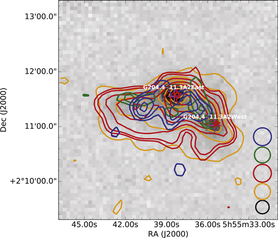
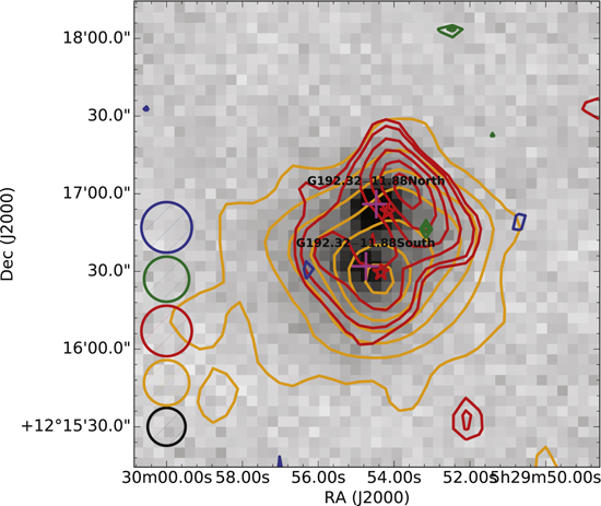
Figure 1. NRO FOREST maps of N2H+ (orange), HC3N (red), CCS-H (green), and CCS-L (blue) integrated intensities overlaid on JCMT SCUBA-2 850 μm continuum emission, in gray scale, for field G204.4. The contours are drawn at 5%, 20%, 35%, 50%, 65%, 80%, and 95% of the peak value above 3σ, and also at 3σ. The respective σ and peak values of the integrated intensity are listed in Table A3. The circles represent the beam sizes with corresponding colors. The black circle, however, corresponds to the SCUBA-2 beam size. The crosses and stars represent a SCUBA-2 core and a protostar, respectively.
Download figure:
Standard image High-resolution image
Figure 2. Same as Figure 1, but for field G206.12.
Download figure:
Standard image High-resolution image
Figure 3. Same as Figure 1, but for field G206.93.
Download figure:
Standard image High-resolution imageTable 3. Map List
| Field | Figure Number |
|---|---|
| G192 | 19.1 |
| G203 | 19.2 |
| G204 | 1 |
| G206.12 | 2 |
| G206.21 | 19.3 |
| G206.93 | 3 |
| G207 | 19.4 |
| G208.68 | 4 |
| G208.89 | 19.5 |
| G209.05 | 19.6 |
| G209.29North | 19.7 |
| G209.29South | 19.8 |
| G209.77 | 19.9 |
| G209.94North | 19.10 |
| G209.94South | 19.11 |
| G210 | 19.12 |
| G211.16 | 5 |
| G211.47 | 6 |
| G211.72 | 19.13 |
| G212 | 7 |
| G159 | 19.14 |
| G171 | 19.15 |
| G172 | 19.16 |
| G173 | 19.17 |
| G178 | 19.18 |
| G006 | 19.19 |
| G001 | 19.20 |
| G17 | 19.21 |
| G14 | 19.22 |
| G16.96 | 19.23 |
| G16.36 | 19.24 |
| G24 | 19.25 |
| G33 | 19.26 |
| G35 | 19.27 |
| G34 | 19.28 |
| G57 | 19.29 |
| G69 | 19.30 |
| G74 | 19.31 |
| G82 | 19.32 |
| G91 | 19.33 |
| G92 | 19.34 |
| G105 | 19.35 |
| G93 | 19.36 |
| G107 | 19.37 |
Download table as: ASCIITypeset image
N2H+ can be destroyed by CO evaporated from the dust in warm environments (Tdust ≳ 25 K) (Jørgensen et al. 2004; Lee et al. 2004; Tatematsu et al. 2014). CCS is basically an early-type molecule, but may have a second abundance enhancement due to the CO depletion before protostar formation (Li et al. 2002; Lee et al. 2003). Occasionally, the CCS distribution surrounds the YSO, which reflects different stages of the chemical evolution, or has an intensity peak toward the YSO position due to locally high excitation. These variations limit the effectiveness of the N2H+/CCS as a chemical evolution tracer in general.
In general, the agreement between the SCUBA-2 cores and N2H+ distribution is good. In some cases, the peak positions of the N2H+ emission and the 850 μm continuum do not coincide with each other. The star-forming core G208.68−19.20North1 (Figure 4; N(DNC)/N(HN13C) = 2.6 ± 1.8, Tbol = 38 ± 13 K, Tkin = 19.7 K) shows such a case. It seems that N2H+ here has been destroyed due to CO evaporated by local heating due to the YSO. This variation limits the effectiveness of N2H+ as a late-type gas tracer in general. Typically, the spatial variation of the N2H+ abundance including chemical evolution will result in a different N2H+ distribution from that of the dust continuum. For example, the southern SCUBA-2 core G211.16–19.33South was detected in the N2H+ emission, but it does not have a prominent peak there. Instead, a prominent N2H+ emission feature is located 1' east of the SCUBA-2 position. This isolated N2H+ feature is an exceptional example in all the fields in this study, however. It is likely that this isolated feature represents a starless core with lower concentration. G211.16–19.33North1, North2 (Tbol = 70 ± 20 K), North4, and North5 (Tbol = 112 ± 16 K), which were detected in both the continuum and N2H+, are star-forming cores. Note that the starless core G211.16–19.33North3 detected in the continuum and N2H+ shows infall motions in ALMA ACA observations (Tatematsu et al. 2020).

Figure 4. Same as Figure 1, but for field G208.68.
Download figure:
Standard image High-resolution imageThe CCS emission shows a clumpy distribution, which is frequently very different from the 850 μm dust continuum distribution, or is simply not detected in most of the cores. The spatial distribution of the line emission is variable from core to core. For the star-forming core G204.4−11.3A2East (Figure 1; N(N2D+)/N(N2H+) = 0.27 ± 0.07), the N2H+ and HC3N lines show a distribution similar to the 850 μm distribution, whereas the CCS-H and -L lines show clumpy distributions, which are very different from the 850 μm distribution. Furthermore, the CCS-L emission appears to surround the dust continuum core, which can be explained in terms of the chemical evolution; the gas in the vicinity of the YSO is more evolved. All four lines are detected in the star-forming core G206.93−16.61West3 (Figure 3) and show distributions similar to the 850 μm distribution. It is possible that local warmer temperatures around the YSO provide high excitation for both the CCS-H and -L emission lines to be detected. The upper energy levels of the CCS-H and CCS-L are 19.9 K and 15.3 K, respectively. Toward the starless cores G206.93−16.61West4 and West5 (Figure 3), we did not detect CCS emission, but only N2H+ emission. Their CEF2.0 values are −27 ± 14 and −34 ± 3, respectively, and they are thought to be evolved starless cores. Furthermore, it is possible that CCS depletion occurs in cold starless cores. The star-forming core G212.10−19.15South (Figure 7, N(N2D+)/N(N2H+) = 0.39 ± 0.06) with a YSO with a low bolometric temperature (Tbol = 43 ± 12 K) does not show any CCS emission. Another YSO with a low bolometric temperature (Tbol = 49 ± 21 K) associated with G211.47−19.27South (Figure 6) does show CCS-H emission, whereas CCS-L emission surrounds it as if it were avoiding the YSO. The YSO associated with G211.16–19.27North1 (Figure 5) accompanies the CCS-L emission, but does not show intense CCS-H emission. We detected both CCS-H and -L emission toward the YSO in G206.93−16.61West3 (Figure 3, N(N2D+)/N(N2H+) = 0.04 ± 0.02, N(DNC)/N(HN13C) = 1.7 ± 1.2). The star-forming core G212.10−19.15North2 (Figure 7) accompanying a YSO having Tbol =114 ± 10 K is associated with CCS-L emission, and also with very weak CCS-H emission. The CCL-H emission has a higher upper energy level (Table 2), but we do not see a very clear tendency that it is more concentrated on the YSO position than the CCS-L emission. 12% of the Orion starless cores show local CCS peak emission toward YSOs in either CCS-H or -L emission.

Figure 5. Same as Figure 1, but for field G211.16.
Download figure:
Standard image High-resolution image
Figure 6. Same as Figure 1, but for field G211.47.
Download figure:
Standard image High-resolution imageThe line detection statistics, line profiles, and column density ratios toward the SCUBA-2 positions are fully presented in our single-pointing paper (Kim et al. 2020). We expect that the telescope error beam will not seriously affect the observed molecular distribution. Because the beam efficiency is high, the line emission distribution is very clumpy, with sizes of ∼1', and the apparent area filling factor of the emission is not very large.
3.2. Line Emission Distribution in Representative Cores
We investigated two extreme cases in detail: case one, G212, in which all the four lines have the same peaks, and case two, G206.12, in which the distributions of the continuum, N2H+, and HC3N emission are different from that of the CCS emission.
First, we considered field G212 (Figure 7). We detect intense emission in CCS-H and -L toward the YSO associated with G212.10−19.15North3 (N(N2D+)/N(N2H+) = 0.06 ± 0.03 and N(DNC)/N(HN13C) = 2.8 ± 2.0). CCS is usually regarded as an early-type gas tracer, but the CCS emission peak coincides with the YSO in this core. In the SCUBA-2 peak G212.10−19.15North1 (N(N2D+)/N(N2H+) = 0.35 ± 0.07), the four molecular lines are all distributed similarly, but their peaks are displaced by ∼40'' or 0.08 pc from the SCUBA-2 peak. It is possible that the YSO is destroying the core. Another possibility is that the YSO has moved from its birth site due to proper motion (Tatematsu et al. 2014), although we do not know the accurate age of the YSO or the vector of its proper motion with respect to the sky plane.

Figure 7. Same as Figure 1, but for field G212.
Download figure:
Standard image High-resolution imageNext, we investigated the radial intensity distribution field G206.12 (Figure 2), which contains only one SCUBA-2 core G206.12−15.76 (N(DNC)/N(HN13C) < 4.8) but was detected with all four lines. This core contains a YSO (Tbol = 35 ± 9 K) near the SCUBA-2 position (29 SSW). We binned the continuum and integrated-intensity line maps to 20'' pixels, which is close to the NRO telescope beam size. Figure 8 compares the intensity normalized for the maximum pixel value in the SCUBA-2 850 μm continuum and the line against the offset from the map center. The values at the same offset from the map center (SCUBA-2 position) were averaged. For the 850 μm continuum, N2H+ and HC3N have their maxima at the core center, which is almost identical to the YSO position. The 850 μm continuum, however, decreases more sharply than those of N2H+ and HC3N. Differences in the telescope beam radius (7'' and 9''–10'' for the 850 μm continuum and the lines, respectively) may affect this difference, but also the molecular lines will be saturated for very high densities, as explained in Section 3. CCS-H and CCS-L seem to have a depression toward the core center. It is known that CCS also exists in evolved molecular gas as a secondary late-stage peak due to CO depletion. The observed emission could represent this gas. It seems that the gas near the core center is more chemically evolved so that the CCS abundance is reduced.
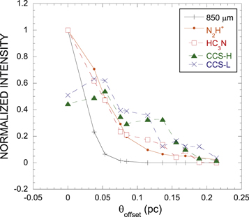
Figure 8. Radial distribution of the continuum and line intensity normalized to the maximum value toward the star-forming core G206.12−15.76 (Figure 2).
Download figure:
Standard image High-resolution image3.3. Physical Properties of the SCUBA-2 Core
We investigated the physical properties of the SCUBA-2 cores using the N2H+ data toward the SCUBA-2 position (Kim et al. 2020). We adopted the hyperfine spectral fitting result for the N2H+ spectrum. We neglected cores with two N2H+ velocity components, as it was difficult to identify the component that corresponded to the SCUBA-2 emission. The nonthermal and total velocity dispersions, σnt and σtot, are defined as in Fuller & Myers (1992),

and

respectively, where Δvobs is the FWHM line width, kB is the Boltzmann constant, and Tkin is the kinetic temperature. We assume that the kinetic temperature is equal to the dust temperature. μobs is the molecular weight of the observed molecule in units of the hydrogen mass mH. The mean molecular weight μ per particle in units of mH is set to 2.33.
In this study, we adopted the HWHM radius R (dust) and mass M (dust) of the core from the SCUBA-2 results of Yi et al. (2018) to avoid uncertainties of the N2H+ abundance. Yi et al. (2018) expressed the core size R in terms of the FWHM diameter, but we express R in terms of the HWHM radius here.
The virial mass Mvir of the uniform-density sphere is derived using the following formula (McKee & Zweibel 1992):

where G is the gravitational constant. The virial parameter αvir is estimated by dividing the virial mass by the SCUBA-2 core mass,

Table 4 lists the velocity dispersion, radius, mass, virial mass, and virial parameter for the SCUBA-2 cores. The virial parameter is as large as ∼5. Figure 9 plots the virial parameter as a function of SCUBA-2 core mass. We adopted the uncertainty in the core radius to be 8% from the uncertainty in the distance adopted by Yi et al. (2018), and derived the uncertainty in the virial parameter assuming the propagation of random errors. From this sample, we obtained the least-squares fit to be αvir ∝ M (dust)−0.7, which can be well described in terms of a pressure-confined core with a form αvir ∝ M−2/3 (Bertoldi & McKee 1992). For the core located near αvir ∼unity, self-gravity is likely to be dominant if we assume that it is in hydrostatic equilibrium. The core with an αvir value that is considerably higher than unity probably needs an appropriate external pressure to bind it if it is not a transient object. Similar results showing large virial parameters are obtained by Kirk et al. (2017) and Kerr et al. (2019) in Orion and in other Gould Belt clouds, respectively. Note that core G211.47−19.27South has a very small virial parameter, αvir = 0.1, and was cataloged by Yi et al. (2018) with an exceptionally small size, which is one order of magnitude smaller than the other cores. Its deconvolved size is smaller than the telescope beam. We define a subcategory of M (dust)  , which seems closer to virial equilibrium. We estimate αvir to be 5.9 ± 4.6 and 2.5 ± 1.2 for all the cores and for the subcategory M (dust)
  , respectively. It should be noted that the virial parameter for the structure embedded in the larger structure can be affected by tidal forces (Mao et al. 2020).
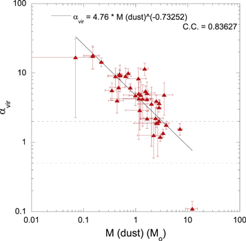
Figure 9. Virial parameter αvir vs. M (dust). The straight line was computed using a least-squares program. C.C represents the correlation coefficient. The horizontal dotted lines represent αvir = 0.5 and 2.
Download figure:
Standard image High-resolution imageTable 4. Physical Properties of N2H+ Core for SCUBA-2 Cores in the Orion Region
| SCUBA-2 core | Δv(N2H+, SCUBA − 2) | σnt | σtot | R(dust) | M(dust) | Mvir | αvir | Tkin | Filament |
|---|---|---|---|---|---|---|---|---|---|
| (km s−1) | (km s−1) | (km s−1) | (pc) | (  ) ) | (  ) ) | (K) | |||
| (1) | (2) | (3) | (4) | (5) | (6) | (7) | (8) | (9) | (10) |
| G192.32−11.88North | 0.66 ± 0.05 | 0.27 ± 0.02 | 0.37 ± 0.03 | 0.030 | 0.49 ± 0.05 | 4.7 ± 0.8 | 9.6 ± 1.7 | 17.3 | N |
| G192.32−11.88South | 0.54 ± 0.02 | 0.22 ± 0.01 | 0.33 ± 0.01 | 0.025 | 0.22 ± 0.02 | 3.2 ± 0.6 | 14.4 ± 2.1 | 17.3 | N |
| G203.21−11.20East1 | 0.76 ± 0.04 | 0.32 ± 0.02 | 0.38 ± 0.02 | 0.060 | 2.50 ± 0.43 | 9.8 ± 1.7 | 3.9 ± 0.8 | 11.2 | Y |
| G203.21−11.20East2 | 0.44 ± 0.03 | 0.18 ± 0.01 | 0.27 ± 0.02 | 0.060 | 2.65 ± 1.73 | 5.0 ± 0.9 | 1.9 ± 1.3 | 11.2 | Y |
| G203.21−11.20West1 | 0.50 ± 0.01 | 0.20 ± 0.01 | 0.29 ± 0.01 | 0.060 | 2.81 ± 0.13 | 5.7 ± 1.0 | 2.0 ± 0.2 | 11.2 | Y |
| G203.21−11.20West2 | 0.50 ± 0.01 | 0.20 ± 0.01 | 0.29 ± 0.01 | 0.050 | 2.51 ± 0.19 | 4.8 ± 0.8 | 1.9 ± 0.3 | 11.2 | Y |
| G204.4−11.3A2East | 0.47 ± 0.01 | 0.19 ± 0.01 | 0.28 ± 0.01 | 0.040 | 2.97 ± 0.23 | 3.5 ± 0.6 | 1.2 ± 0.2 | 11.1 | N |
| G204.4−11.3A2West | 0.83 ± 0.06 | 0.35 ± 0.03 | 0.40 ± 0.03 | 0.025 | 0.99 ± 0.24 | 4.7 ± 0.8 | 4.7 ± 1.3 | 11.1 | N |
| G206.93−16.61West1 | 0.84 ± 0.03 | 0.35 ± 0.01 | 0.43 ± 0.02 | 0.040 | 1.55 ± 0.23 | 8.5 ± 1.5 | 5.5 ± 1.0 | 16.8 | Y |
| G206.93−16.61West3 | 0.65 ± 0.04 | 0.27 ± 0.02 | 0.36 ± 0.02 | 0.030 | 3.38 ± 0.15 | 4.6 ± 0.8 | 1.4 ± 0.2 | 16.8 | Y |
| G206.93−16.61West4 | 0.64 ± 0.04 | 0.26 ± 0.02 | 0.36 ± 0.02 | 0.040 | 1.25 ± 0.67 | 6.0 ± 1.0 | 4.8 ± 2.7 | 16.8 | Y |
| G206.93−16.61West5 | 0.81 ± 0.07 | 0.34 ± 0.03 | 0.42 ± 0.04 | 0.055 | 7.10 ± 0.72 | 11.1 ± 1.9 | 1.6 ± 0.3 | 16.8 | Y |
| G206.93−16.61West6 | 0.62 ± 0.07 | 0.25 ± 0.03 | 0.35 ± 0.04 | 0.040 | 1.15 ± 0.15 | 5.8 ± 1.0 | 5.0 ± 1.2 | 16.8 | Y |
| G207.36−19.82North1 | 1.13 ± 0.04 | 0.48 ± 0.02 | 0.52 ± 0.02 | 0.030 | 1.13 ± 0.46 | 9.4 ± 1.6 | 8.3 ± 3.5 | 11.9 | Y |
| G207.36−19.82North2 | 0.45 ± 0.02 | 0.18 ± 0.01 | 0.27 ± 0.01 | 0.020 | 0.44 ± 0.14 | 1.8 ± 0.3 | 4.0 ± 1.4 | 11.9 | Y |
| G207.36−19.82North3 | 0.69 ± 0.04 | 0.29 ± 0.02 | 0.35 ± 0.02 | 0.020 | 0.47 ± 0.15 | 2.9 ± 0.5 | 6.2 ± 2.1 | 11.9 | Y |
| G207.36−19.82North4 | 0.80 ± 0.06 | 0.33 ± 0.03 | 0.39 ± 0.03 | 0.015 | 0.15 ± 0.05 | 2.7 ± 0.5 | 18.0 ± 6.5 | 11.9 | Y |
| G207.36−19.82South | 0.38 ± 0.16 | 0.15 ± 0.06 | 0.26 ± 0.11 | 0.095 | 2.01 ± 0.91 | 7.2 ± 1.2 | 3.6 ± 2.7 | 11.9 | N |
| G208.68−19.20North2 | 0.42 ± 0.01 | 0.16 ± 0.01 | 0.31 ± 0.01 | 0.025 | 2.22 ± 1.15 | 2.8 ± 0.5 | 1.3 ± 0.7 | 19.7 | Y |
| G208.89−20.04East | 0.38 ± 0.01 | 0.14 ± 0.01 | 0.30 ± 0.01 | 0.065 | 3.86 ± 0.29 | 6.9 ± 1.2 | 1.8 ± 0.2 | 19.7 | N |
| G209.05−19.73North | 0.38 ± 0.02 | 0.15 ± 0.01 | 0.28 ± 0.01 | 0.115 | 2.83 ± 0.15 | 10.3 ± 1.8 | 3.6 ± 0.5 | 15.6 | Y |
| G209.05−19.73South | 0.43 ± 0.03 | 0.17 ± 0.01 | 0.29 ± 0.02 | 0.070 | 1.65 ± 0.29 | 6.9 ± 1.2 | 4.2 ± 0.9 | 15.6 | Y |
| G209.29−19.65South1 | 1.42 ± 0.04 | 0.60 ± 0.02 | 0.65 ± 0.02 | 0.035 | 1.49 ± 0.26 | 17.1 ± 3.0 | 11.5 ± 2.4 | 17.3 | Y |
| G209.29−19.65South3 | 0.66 ± 0.03 | 0.27 ± 0.01 | 0.37 ± 0.02 | 0.030 | 0.50 ± 0.05 | 4.7 ± 0.8 | 9.4 ± 1.5 | 17.3 | Y |
| G209.77−19.40East1 | 0.35 ± 0.01 | 0.13 ± 0.01 | 0.26 ± 0.01 | 0.025 | 0.35 ± 0.09 | 2.0 ± 0.3 | 5.6 ± 1.6 | 13.9 | Y |
| G209.77−19.40East2 | 0.47 ± 0.01 | 0.19 ± 0.01 | 0.29 ± 0.01 | 0.035 | 1.20 ± 0.56 | 3.5 ± 0.6 | 2.9 ± 1.4 | 13.9 | Y |
| G209.94−19.52North | 0.60 ± 0.01 | 0.25 ± 0.01 | 0.34 ± 0.01 | 0.065 | 2.81 ± 0.28 | 8.9 ± 1.5 | 3.2 ± 0.5 | 16.3 | N |
| G210.82−19.47North1 | 0.44 ± 0.01 | 0.17 ± 0.01 | 0.30 ± 0.01 | 0.070 | 0.72 ± 0.08 | 7.2 ± 1.2 | 10.0 ± 1.5 | 16.2 | Y |
| G210.82−19.47North2 | 0.35 ± 0.01 | 0.13 ± 0.01 | 0.27 ± 0.01 | 0.030 | 0.15 ± 0.05 | 2.6 ± 0.5 | 17.5 ± 6.1 | 16.2 | Y |
| G211.16–19.33North1 | 0.44 ± 0.02 | 0.18 ± 0.01 | 0.28 ± 0.01 | 0.055 | 0.79 ± 0.05 | 4.9 ± 0.8 | 6.1 ± 0.8 | 12.5 | Y |
| G211.16–19.33North2 | 0.46 ± 0.01 | 0.19 ± 0.01 | 0.28 ± 0.01 | 0.050 | 0.50 ± 0.20 | 4.6 ± 0.8 | 9.2 ± 3.8 | 12.5 | Y |
| G211.16–19.33North3 | 0.35 ± 0.01 | 0.14 ± 0.01 | 0.25 ± 0.01 | 0.050 | 0.41 ± 0.12 | 3.7 ± 0.6 | 8.9 ± 2.8 | 12.5 | Y |
| G211.16–19.33North5 | 0.48 ± 0.01 | 0.19 ± 0.01 | 0.29 ± 0.01 | 0.060 | 0.64 ± 0.18 | 5.8 ± 1.0 | 9.0 ± 2.7 | 12.5 | Y |
| G211.47−19.27North | 0.52 ± 0.01 | 0.21 ± 0.01 | 0.30 ± 0.01 | 0.035 | 1.66 ± 0.43 | 3.6 ± 0.6 | 2.2 ± 0.6 | 12.4 | N |
| G211.47−19.27South | 1.03 ± 0.03 | 0.43 ± 0.01 | 0.48 ± 0.01 | 0.005 | 12.25 ± 3.18 | 1.3 ± 0.2 | 0.1 ± 0.03 | 12.4 | N |
| G211.72−19.25North | 0.38 ± 0.02 | 0.15 ± 0.01 | 0.26 ± 0.01 | 0.015 | 0.07 ± 0.06 | 1.2 ± 0.2 | 16.8 ± 14.5 | 12.6 | Y |
| G211.72−19.25South1 | 0.40 ± 0.05 | 0.16 ± 0.02 | 0.26 ± 0.03 | 0.060 | 1.15 ± 0.82 | 4.9 ± 0.8 | 4.3 ± 3.2 | 12.6 | Y |
| G212.10−19.15North1 | 0.84 ± 0.04 | 0.35 ± 0.02 | 0.40 ± 0.02 | 0.090 | 3.52 ± 1.68 | 17.0 ± 2.9 | 4.8 ± 2.4 | 10.8 | Y |
| G212.10−19.15North2 | 0.69 ± 0.02 | 0.29 ± 0.01 | 0.35 ± 0.01 | 0.060 | 1.65 ± 0.72 | 8.5 ± 1.5 | 5.1 ± 2.3 | 10.8 | Y |
| G212.10−19.15North3 | 0.55 ± 0.05 | 0.23 ± 0.02 | 0.30 ± 0.03 | 0.055 | 1.36 ± 0.78 | 5.8 ± 1.0 | 4.2 ± 2.5 | 10.8 | Y |
| G212.10−19.15South | 0.38 ± 0.01 | 0.15 ± 0.01 | 0.25 ± 0.01 | 0.075 | 2.41 ± 1.00 | 5.4 ± 0.9 | 2.2 ± 1.0 | 10.8 | Y |
| Mean (All) | 0.59 ± 0.23 | 0.24 ± 0.10 | 0.33 ± 0.08 | 0.047 ± 0.023 | 1.90 ± 2.14 | 5.9 ± 3.6 | 5.9 ± 4.6 | 13.9 ± 2.7 | |
| Median (All) | 0.50 | 0.20 | 0.30 | 0.040 | 1.36 | 4.9 | 4.7 | 12.5 | |
| Mean (Starless) | 0.64 ± 0.11 | 0.26 ± 0.11 | 0.35 ± 0.09 | 0.048 ± 0.025 | 1.81 ± 1.53 | 6.8 ± 4.1 | 5.8 ± 4.5 | ||
| Median (Starless) | 0.63 | 0.26 | 0.35 | 0.040 | 1.37 | 5.4 | 4.5 | ||
| Mean (Star-forming) | 0.51 ± 0.16 | 0.21 ± 0.07 | 0.31 ± 0.05 | 0.045 ± 0.021 | 2.03 ± 2.84 | 4.6 ± 2.0 | 6.0 ± 4.8 | ||
| Median (Star-forming) | 0.48 | 0.19 | 0.30 | 0.050 | 1.36 | 4.8 | 5.1 | ||
Note. Column 1: SCUBA-2 core name. Column 2: N2H+ FWHM line width toward the SCUBA-2 position (Kim et al. 2020). Column 3: nonthermal velocity dispersion. Column 4: total velocity dispersion. Column 5: HWHM dust continuum radius (Yi et al. 2018). Column 6: mass from the dust continuum (Yi et al. 2018). Column 7: virial mass. Column 8: virial parameter. Column 9: kinetic temperature. Column 10: association with the filament.
Download table as: ASCIITypeset image
3.4. Line Emission Distribution of the Orion Core
We statistically compared the emission distributions of the four lines on the basis of their integrated-intensity maps toward Orion cores. We selected the emission feature that was approximately coincident with the SCUBA-2 850 μm dust continuum emission through visual inspection and fitted a two-dimensional Gaussian to it. We identified the most prominent feature that was nearest to the SCUBA-2 position. Although this description may sound somewhat imprecise, the identification is practically straightforward.
The individual core data are listed in Tables A4 and A5 in the Appendix. Table 5 summarizes statistics for the offset θoffset of the Gaussian-fit center from the SCUBA-2 position and the beam deconvolved radius R of the fit. Note that the offset of CCS-L is twice as large as the offsets of N2H+ and CCS-H. Therefore, CCS-L emission is in general less correlated with the SCUBA-2 emission. We did not observe large differences in radius between the lines.
Table 5. Line Emission Distribution Summary in the Orion Region
| SCUBA-2 core | N2H+ | HC3N | CCS-H | CCS-L | ||||
|---|---|---|---|---|---|---|---|---|
| θoffset | R | θoffset | R | θoffset | R | θoffset | R | |
| (pc) | (pc) | (pc) | (pc) | (pc) | (pc) | (pc) | (pc) | |
| (1) | (2) | (3) | (4) | (5) | (6) | (7) | (8) | (9) |
| mean | 0.027 | 0.073 | 0.031 | 0.065 | 0.021 | 0.062 | 0.045 | 0.081 |
| stdev | 0.026 | 0.027 | 0.036 | 0.026 | 0.022 | 0.027 | 0.041 | 0.040 |
Note. Column 1: calculation. Column 2: offset of the N2H+ emission from the SCUBA-2 position in parsecs. Column 3: deconvolved radius of the N2H+ emission in parsecs. Column 4: offset of the HC3N emission from the SCUBA-2 position in parsecs. Column 5: deconvolved radius of HC3N emission in parsecs. Column 6: offset of the CCS-H emission from the SCUBA-2 position in parsecs. Column 7: deconvolved radius of the CCS-H emission in parsecs. Column 8: offset of the CCS-L emission from the SCUBA-2 position in parsecs. and Column 9: deconvolved radius of CCS-L emission in parsecs.
Download table as: ASCIITypeset image
We also illustrate the offset and emission radius by a histogram. Figure 10 provides a comparison of the offset of the line emission fitted ellipse center from the SCUBA-2 position for the Orion cores. The offsets in N2H+ and HC3N are similarly distributed, having sharp peaks at θoffset = 0–0.02 pc. These offsets are not significant, because 0.02 pc approximately corresponds to half the NRO beam size. The offsets in CCS-H and CCS-L appear to be less peaked. Figure 11 shows a comparison of the deconvolved radius values of the line emission feature for the Orion cores, in which no significant differences among the lines are observed.
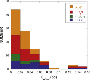
Figure 10. Histogram of the line emission offset from the SCUBA-2 position. Statistics are listed in Table 5.
Download figure:
Standard image High-resolution image
Figure 11. Histogram of the deconvolved radius R for each line. Statistics are listed in Table 5.
Download figure:
Standard image High-resolution image3.5. Comparison Between the Starless and Star-forming Cores in the Orion Region
At the bottom of Table 4, we list parameter statistics for all the cores together and for starless and star-forming cores separately. The starless and star-forming cores have very similar radii, suggesting no evolutionary change in the core radius is detected at 0.027 pc linear resolution. Furthermore, their nonthermal velocity dispersions, masses, and virial masses are not appreciably different. Therefore no evidence for the dissipation of turbulence is identified at the employed spatial resolution, as already noted by Kim et al. (2020). The absence of differences in the velocity dispersion between the starless and star-forming cores contradicts the results of earlier studies (Beichman et al. 1986; Benson & Myers 1989; Zhou et al. 1989; Tatematsu et al. 1993). One possibility is that largely improved sensitivities allow the identification of low-luminosity YSOs that were previously undetectable. To test this possibility, we plotted the nonthermal velocity dispersion against the bolometric luminosity of the YSO taken from Dutta et al. (2020; Figure 12). Except for the core with the most luminous YSO (G211.47−19.27South, L = 180 ± 70  ), no clear positive correlation was observed. Our data were less affected by star formation activities because the tracer N2H+ employed is insensitive to shocked gas (Turner & Thaddeus 1977; Womack et al. 1993; Bachiller 1996; Caselli et al. 2002), unlike CS and NH3 employed in previous studies. Our samples contain warm Tbol YSOs, which are not too young to observe the impacts of YSO activities.
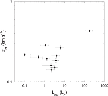
Figure 12. Nonthermal velocity dispersion vs. bolometric luminosity of the YSO (Dutta et al. 2020).
Download figure:
Standard image High-resolution imageWe also compared the deconvolved radii (Yi et al. 2018) between the starless and star-forming cores. Figure 13 shows the histogram of the SCUBA-2 radius R (dust) of the two categories. The starless and star-forming cores have very similar radii. We corrected the semimajor axis a and semiminor axis b for the telescope beam in quadrature, and calculated the deconvolved radius R,


Figure 13. Histogram of the deconvolved radii of the SCUBA-2 cores in the Orion region. Black and orange indicate the starless and star-forming cores, respectively. The vertical solid line represents the telescope beam radius.
Download figure:
Standard image High-resolution imageThe SCUBA-2 beam radius is 7'' or 0.0135 pc; thus, the cores are well resolved. This similarity is not consistent with the result from H13CO+ observations toward Taurus by Mizuno et al. (1994), who concluded that starless cores are larger than star-forming cores, but it is consistent with that from N2H+ observations by Tatematsu et al. (2004) for the same cores. A possible reason for this difference is the depletion of H13CO+ molecules in the starless cores, which could cause flat-topped radial intensity profiles toward cold starless cores, and correspondingly lead to larger radii (Tatematsu et al. 2004). It seems that when we use a molecular-line tracer affected by depletions we see a size difference between the starless and star-forming cores. In contrast, when we use the dust continuum or a tracer that is less affected by depletion, it seems difficult to observe differences in radii with HPBWs of 0.01−0.03 pc. When we adopt Welch's t-test for the null hypothesis that the starless and star-forming cores have equal radii, we obtain a p-value of 0.55, which is considerably higher than a standard threshold of 0.05 for statistical significance. Thus, we cannot statistically conclude that these two categories have different radii.
It is suggested that the sizes of identified cores are often very close to the telescope beam size, and this can be well explained if cores have power-law density profiles. Ladd et al. (1991) indicated that the observed emission size tends to be 10−80% larger than the original beam size if we assume the power-law radial intensity distribution. Young et al. (2003) showed an anticorrelation between the power-law index and the deconvolved emission size (see their Figure 27). Then, in these cases, the observed radius represents the radial density slope rather than the physical boundary. The mean HWHM radius (230 ± 114 or 0.045 ± 0.022 pc) and beam radius (7'' or 0.0135 pc) suggest a power-law index p of <1.4 for the radial density profile ρ (r) ∝ r−p
. Therefore the SCUBA-2 core in Orion studied by Yi et al. (2018) arguably has a shallow radial density profile.
4. Discussion
4.1. Physical Parameters of the Starless Cores Against CEF2.0
We investigated how the physical parameters of the starless cores compare to evolutionary indications based on chemistry, as encoded by CEF2.0, which is the chemical evolution tracer based on the deuterium fraction. Table 6 lists the deuterium fraction and CEF2.0 for all cores observed. Note that CEF2.0 is defined only for the starless cores in Orion, but this table contains the starless and star-forming cores, and also the cores outside Orion. Kim et al. (2020) pointed out that the deuterium fraction will be seriously underestimated for distant (>1 kpc) cores due to beam dilution. The adopted distance is listed in Table A1. Table A2 in the appendix contains the YSO association information. The CEF2.0 values of the Orion starless cores were calculated from the column density ratios of N2D+/N2H+ and DNC/HN13C from our single-pointing observations (Kim et al. 2020). We question whether there is any evidence that stable cores change into unstable cores by changing physical properties such as turbulence.
Table 6. Deuterium Fraction and CEF2.0
| SCUBA-2 Core | VLSR | N(N2D+)/N(N2H+) | N(DNC)/N(HN13C) | YSO | CEF2.0 |
|---|---|---|---|---|---|
| (km s−1) | |||||
| G192.32−11.88North | 12.1 | 0.15 ± 0.08 | 5.2 ± 3.7 | Y | |
| G192.32−11.88South | 12.2 | 0.17 ± 0.02 | 3.8 ± 2.7 | Y | |
| G203.21−11.20West1 | 10.7 | 0.30 ± 0.04 | <4.1 | Y | |
| G203.21−11.20West2 | 10.2 | 0.21 ± 0.05 | <4.0 | Y | |
| G204.4−11.3A2East | 1.6 | 0.27 ± 0.07 | <4.2 | Y | |
| G204.4−11.3A2West | 1.7 | 0.09 ± 0.04 | ⋯ | Y | |
| G206.12−15.76 | 8.5 | ⋯ | <4.8 | Y | |
| G206.93−16.61West1 | 9.3 | <0.15 | 1.0 ± 0.7 | Y | |
| G206.93−16.61West3 | 9.3 | 0.04 ± 0.02 | 1.7 ± 1.2 | Y | |
| G206.93−16.61West4 | 10.1 | 0.16 ± 0.04 | 5.1 ± 3.7 | N | −27 ± 14 |
| G206.93−16.61West5 | 9.0 | 0.15 ± 0.02 | ⋯ | N | −34 ± 3 |
| G206.93−16.61West6 | 10.4 | <0.23 | 2.7 ± 1.9 | Y | |
| G207.36−19.82North2 | 11.2 | 0.22 ± 0.05 | <6.8 | Y | |
| G207.36−19.82South | 11.3 | 0.11 ± 0.04 | ⋯ | N | −41 ± 8 |
| G208.68−19.20North1 | 11.1 | <0.08 | 2.6 ± 1.8 | Y | |
| G208.68−19.20North2 | 11.2 | 0.11 ± 0.01 | 3.1 ± 2.2 | Y | |
| G208.68−19.20North3 | 11.1 | 0.06 ± 0.01 | 2.7 ± 1.9 | Y | |
| G209.05−19.73North | 8.3 | 0.27 ± 0.06 | 5.7 ± 4.2 | N | −19 ± 15 |
| G209.05−19.73South | 7.9 | 0.23 ± 0.13 | 5.9 ± 4.4 | N | −20 ± 19 |
| G209.29−19.65North1 | 8.6 | 0.06 ± 0.03 | 2.0 ± 1.4 | N | −58 ± 17 |
| G209.29−19.65South1 | 7.5 | 0.11 ± 0.02 | ⋯ | N | −42 ± 5 |
| G209.29−19.65South2 | 7.8 | <0.08 | 3.4 ± 2.5 | N | −38 ± 36 |
| G209.29−19.65South2 | 9.0 | 0.14 ± 0.08 | 0.7 ± 0.5 | N | −67 ± 18 |
| G209.77−19.40East1 | 8.1 | 0.05 ± 0.01 | 1.8 ± 1.3 | Y | |
| G209.77−19.40East2 | 8.0 | <0.14 | 2.5 ± 1.8 | N | −50 ± 27 |
| G209.77−19.40East3 | 7.8 | 0.25 ± 0.04 | 4.7 ± 3.4 | N | −23 ± 14 |
| G209.77−19.40East3 | 8.3 | <0.63 | 1.9 ± 1.4 | N | −61 ± 28 |
| G209.94−19.52North | 8.1 | 0.33 ± 0.07 | 3.6 ± 2.5 | Y | |
| G209.94−19.52South1 | 7.5 | 0.24 ± 0.13 | 6.3 ± 4.5 | N | −18 ± 15 |
| G209.94−19.52South1 | 8.1 | 0.24 ± 0.03 | 4.1 ± 2.9 | N | −26 ± 14 |
| G210.82−19.47North1 | 5.3 | 0.32 ± 0.03 | 4.0 ± 2.9 | Y | |
| G210.82−19.47North2 | 5.3 | 0.20 ± 0.02 | 5.3 ± 3.8 | N | −24 ± 14 |
| G211.16–19.33North2 | 3.7 | 0.10 ± 0.04 | <2.5 | Y | |
| G211.16–19.33North3 | 3.4 | 0.24 ± 0.05 | <3.5 | N | −22 ± 5 |
| G211.16–19.33North5 | 4.3 | 0.31 ± 0.06 | <3.2 | Y | |
| G211.47−19.27North | 4.1 | 0.10 ± 0.02 | <3.1 | Y | |
| G212.10−19.15North1 | 4.3 | 0.35 ± 0.07 | <6.1 | Y | |
| G212.10−19.15North3 | 4.2 | 0.06 ± 0.03 | 2.8 ± 2.0 | Y | |
| G212.10−19.15South | 3.9 | 0.39 ± 0.06 | <3.5 | Y | |
| SCOPEG159.18−20.09 | 6.3 | ⋯ | 13.8 ± 9.7 | Y | |
| SCOPEG159.22−20.11 | 6.7 | ⋯ | 10.5 ± 7.5 | Y | |
| SCOPEG173.17 + 02.36 | −18.9 | ⋯ | 1.1 ± 0.8 | Y | |
| SCOPEG173.18 + 02.35 | −19.0 | ⋯ | 1.3 ± 0.9 | Y | |
| SCOPEG173.19 + 02.35 | −19.3 | ⋯ | 1.6 ± 1.2 | Y | |
| SCOPEG001.37 + 20.95 | 0.8 | ⋯ | 14.6 ± 10.3 | N | |
| SCOPEG017.38 + 02.26 | 10.7 | ⋯ | 1.7 ± 1.3 | Y | |
| SCOPEG017.37 + 02.24 | 10.5 | ⋯ | 1.1 ± 0.8 | Y | |
| SCOPEG017.36 + 02.23 | 10.4 | ⋯ | 0.6 ± 0.4 | Y | |
| SCOPEG014.18−00.23 | 40.5 | ⋯ | 1.1 ± 0.8 | Y | |
| SCOPEG016.93 + 00.25 | 24.2 | ⋯ | 2.3 ± 1.6 | N | |
| SCOPEG016.93 + 00.24 | 24.3 | ⋯ | 0.6 ± 0.4 | N | |
| SCOPEG016.93 + 00.24 | 26.3 | ⋯ | 0.8 ± 0.6 | N | |
| SCOPEG016.93 + 00.22 | 23.6 | ⋯ | 1.4 ± 1.0 | Y | |
| SCOPEG033.74−00.01 | 105.0 | ⋯ | 0.4 ± 0.3 | Y | |
| SCOPEG035.48−00.29 | 45.3 | ⋯ | 1.8 ± 1.3 | Y | |
| SCOPEG035.52−00.27 | 45.1 | ⋯ | 1.6 ± 1.1 | Y | |
| SCOPEG035.48−00.31 | 44.9 | ⋯ | 1.6 ± 1.1 | Y | |
| SCOPEG034.75−01.38 | 45.6 | ⋯ | 0.9 ± 0.6 | Y | |
| SCOPEG069.80−01.67 | 12.4 | ⋯ | 1.2 ± 0.8 | Y | |
| SCOPEG069.81−01.67 | 12.1 | ⋯ | 1.2 ± 0.9 | Y | |
| SCOPEG105.37 + 09.84 | −9.7 | ⋯ | 1.8 ± 1.3 | Y | |
| SCOPEG107.16 + 05.45 | −10.2 | ⋯ | 5.5 ± 3.9 | Y | |
| SCOPEG107.18 + 05.43 | −10.8 | ⋯ | 1.8 ± 1.3 | Y |
Download table as: ASCIITypeset image
Figure 14 shows the plot of the nonthermal velocity dispersion, radius, H2 column density, mass, and virial parameter of the Orion starless cores against CEF2.0, in which no significant trend observed. Radius R and mass M increase with increasing CEF2.0 from CEF2.0 = −24 to −19, but this rise is probably not significant when we take the error in CEF2.0 into account. The virial parameter αvir of the starless cores is as large as 1−20. If we allow 1σ uncertainty, four cores (44%) out of the nine starless cores in this figure may fit the range 0.5 < αvir < 2. Large virial parameters for starless cores suggest that most of them are either pressure confined or transient. Chen et al. (2020) showed the evolution of unbound cores into bound cores in their simulation.

Figure 14. Nonthermal velocity dispersions, radii, H2 column densities, masses, and virial parameters of the starless cores vs. CEF2.0. The core radii, column densities, and masses are taken from Yi et al. (2018). The error bar for CEF2.0 is plotted only for the nonthermal velocity dispersion for clarity.
Download figure:
Standard image High-resolution imageCrapsi et al. (2005) noted that the chemical properties (including the deuterium fraction) and physical properties (density, line width, etc.) of starless cores as a whole can trace the evolutionary stage, although they did not find very tight dependences between these properties. Their samples included starless cores at younger stages such as B68, TMC-1, L492, L1498, and L1512 (Shirley et al. 2005; Hirota & Yamamoto 2006), which have values of −100 ≲ CEF2.0 ≲ −60 (Kim et al. 2020), implying lower deuterium fractions. They concluded that evolved starless cores with higher N(N2D+)/N(N2H+) tend to have higher central H2 column densities and more compact density profiles. They employed multiple tracers including N2H+, N2D+, and the dust continuum emission, and the above physical parameters were derived at linear resolutions of 0.006−0.02 pc, 1.5−6 times better than our linear resolution (0.03−0.04 pc). The difference in the linear resolution and/or the CEF2.0 range may at least partially explain the difference in conclusion.
Marka et al. (2012) observed Bok globules in NH3 and CCS to study their chemical evolution. They did not find any globules with extremely high CCS abundances and concluded that all of the observed Bok globules are in a relatively evolved chemical state. It is possible that the SCUBA-2 cores with high column densities selected in our study are similarly biased to evolved cores.
We did not observe intense CCS emission even at the starless core stage. Relatively late chemical evolution stages may be one reason, but we also suspect that serious depletion occurs in CCS at cold starless cores, which leads to the low values of the CCS column density. Some previous studies of core chemistry evolution used the abundance at the molecular line emission maximum (Ohashi et al. 2014; Tatematsu et al. 2014), which can be different from that at density peaks traced by the dust continuum emission. In these cases, the depletion of CCS can be alleviated. We used the SCUBA-2 position as the core centers where the CCS depletion could be severe.
4.2. Core Evolution against the Bolometric Temperature
We investigated the physical parameters of the star-forming cores against the bolometric temperature of associated YSOs (Dutta et al. 2020). The bolometric temperature is a reliable empirical tracer of star-forming core's evolution (Chen et al. 1995). The bolometric temperature Tbol can be obtained from the flux-weighted mean frequencies in the observed spectral energy distributions (SEDs; Myers & Ladd 1993). Dutta et al. (2020) used their ALMA 1.3 mm fluxes as well as fluxes at other wavelengths from Cutri et al. (2003), Lawrence et al. (2007), Wright et al. (2010), Megeath et al. (2012), Stutz et al. (2013), Tobin et al. (2015), Doi et al. (2015), and Yi et al. (2018). Figure 15 shows the nonthermal velocity dispersion, radius, H2 column density, mass, and virial parameter versus Tbol for the star-forming cores (Dutta et al. 2020). We did not observe any significant trends in this figure. The virial parameter αvir of the star-forming core ranged from 0.1 to 20. Six (55%) of the eleven star-forming cores in this figure may fit the range αvir = 0.5–2 when we allow a 1σ uncertainty. The core that forms a protostar should be gravitationally bound or pressure confined at least when the protostar forms. Large virial parameters of the star-forming core suggest either a confining external pressure, a fast core dispersal after star formation, strong tidal forces from the ambient gas, or systematic bias in the estimation of the parameter. Furthermore, the associated outflow can stir up the core to some extent through magnetic fields, although N2H+ is less affected by shocks.

Figure 15. Nonthermal velocity dispersions, radii, H2 column densities, masses, and virial parameters of the star-forming cores vs. bolometric temperatures Tbol of the YSOs (Dutta et al. 2020). The error bar for Tbol is plotted only for the nonthermal velocity dispersion for clarity.
Download figure:
Standard image High-resolution imageWe also investigated the distribution of CCS (young-gas tracer) and N2H+ (evolved-gas tracer) versus Tbol . Figure 16 shows the close-up maps of representative star-forming cores aligned in order of the bolometric temperature Tbol of the associated YSO as an evolutionary tracer for star-forming cores. Comparisons including HC3N on the full-sized maps of the all star-forming Orion cores with Tbol can be seen with Table A2, Figures 1– 7, and Figure Set 19. Again, no clear trend is seen.

Figure 16. Close-up maps sorted in order of evolutionary stages using Tbol for representative star-forming cores. Each map represents the integrated-intensity contour map superposed on the 850 μm dust continuum emission map. The orange, green, and blue contours represent the N2H+, CCS-H, and CCS-L integrated-intensity contour maps, respectively. The innermost to outermost contour levels correspond to 95%, 80%, 65%, 50%, 35%, 20%, 5%, and 3σ, respectively. The σ and peak values of integrated intensity are listed in Table A3. The cross and stars represent a SCUBA-2 core and a protostar, respectively. The error for Tbol is listed in Table A2 in the appendix.
Download figure:
Standard image High-resolution image4.3. Relation with the Association with the Filament
Some of the observed cores are apparently located in filaments. Because filaments likely play an important role in inflow into cores, we investigate whether there are any differences between cores inside or outside filaments. The association with a filament was judged from the SCUBA-2 and N2H+ distributions is shown in Table 4. Table 7 summarizes the statistics of the Orion core. Here, we do not distinguish the starless and star-forming cores. The nonthermal velocity dispersions and radii are similar between the two categories. The cores associated with filaments are slightly less massive and have smaller virial parameters, although the standard deviation is large and so the differences may not be significant.
Table 7. Core Properties with and without the Filaments
| Filament | Calculation | σnt | R (dust) | M (dust) | αvir |
|---|---|---|---|---|---|
| (km s−1) | (pc) | (  ) ) | |||
| Y | mean | 0.24 ± 0.11 | 0.05 ± 0.02 | 1.58 ± 1.41 | 6.29 ± 4.56 |
| Y | median | 0.20 | 0.05 | 1.23 | 4.93 |
| N | mean | 0.25 ± 0.09 | 0.04 ± 0.03 | 3.03 ± 3.66 | 4.54 ± 4.62 |
| N | median | 0.22 | 0.04 | 2.01 | 3.18 |
Download table as: ASCIITypeset image
4.4. Kinematics
Details of the kinematics of the cores discussed here are beyond the scope of this paper, but we consider here two example fields, each containing representative examples, G206.12 and G211.16. We selected them from Orion cores, as they have more accurate distances (Kounkel et al. 2017; Perryman et al. 1997), and they are less affected by beam dilution (Kim et al. 2020).
One field, G206.12, has only one SCUBA-2 core inside the mapped area (Figure 2), whereas the other field, G211.16, contains six SCUBA-2 cores (Figure 5). The N2H+ emission was used for the analysis. We calculated the intensity-weighted radial velocity (moment 1) using the hyperfine group J = 1 → 0 F1 = 2 → 1 containing the brightest hyperfine component to obtain better signal-to-noise ratios (S/Ns), and the velocity dispersion (moment 2) using the isolated hyperfine component J = 1 → 0, F1, F = 0, 1 → 1, 2, which is optically thinner and less affected by the neighboring satellites.
Field G206.12 (Figure 17) does not exhibit any significant velocity gradients. The velocity dispersion seems to increase toward the core center harboring the YSO. This shift may represent the influence from the YSO. In field G211.16 (Figure 18), however, the velocity field shows distinct velocities for filaments.
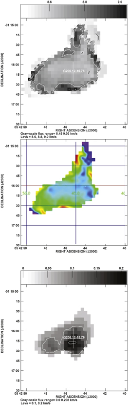
Figure 17. The top and middle panels show the intensity-weighted velocity (moment 1) maps in gray scale and in pseudo-color, respectively, toward field G206.12 (Figure 2). The bottom panel shows the intensity-weighted velocity dispersion (moment 2) map in gray scale toward the same field.
Download figure:
Standard image High-resolution image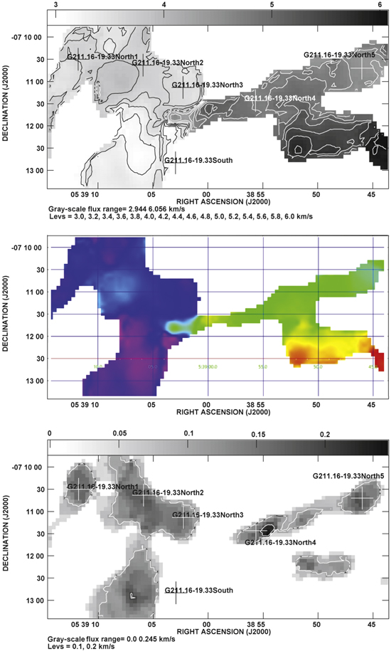
Download figure:
Standard image High-resolution image5. Summary
We performed OTF mapping observations of 44 fields containing 107 SCUBA-2 cores in the N2H+, HC3N, 94 GHz CCS, and 82 GHz CCS lines using the Nobeyama 45 m telescope. The distribution of N2H+ and HC3N line emission is similar to the respective 850 μm distribution, whereas CCS lines are undetected or distributed in clumpy structures surrounding the peak position of the 850 μm dust continuum emission. Occasionally (12%), we detected the CCS emission, which is considered an early-type gas tracer, toward YSOs. The nonthermal velocity dispersions of the SCUBA-2 cores in Orion are very similar between the starless and star-forming core populations, suggesting that evolution toward star formation does not immediately affect the nonthermal velocity dispersion.
K.T. and T.S. were supported by JSPS KAKENHI grant No. 20H05645. T.L. acknowledges the supports from the international partnership program of the Chinese Academy of Sciences (CAS) through grant No. 114231KYSB20200009, the National Natural Science Foundation of China (NSFC) through grant NSFC No. 12073061, and the Shanghai Pujiang Program 20PJ1415500. N.H. acknowledges a grant from the Ministry of Science and Technology (MoST) of Taiwan (MoST109-2112-M-001-023- and MoST 110-2112-M-001-048-). P.S. was partially supported by a Grant-in-Aid for Scientific Research (KAKENHI No. 18H01259) of JSPS. J.H. thanks NSFC under grant Nos. 11873086 and U1631237 and acknowledges support by the Yunnan Province of China (No. 2017HC018), and his work is sponsored in part by CAS through a grant to the CAS South America Center for Astronomy (CASSACA) in Santiago, Chile. J.G. acknowledges the support from CAS through a Postdoctoral Fellowship administered by CASSACA in Santiago, Chile.
Facility: No:45m. -
Software: AIPS (van Moorsel et al. 1996), APLpy (Robitaille & Bressert 2012), Astropy (Astropy Collaboration et al. 2013, 2018), NOSTAR (Sawada et al. 2008), SAOImageDS9 (Joye & Mandel 2003), spectral-cube (Robitaille et al. 2016).
Appendix: Maps
Tables A1 and A2 summarize the field name, map-center coordinates, map size, distance, region, SCUBA-2 core name, core coordinates, name of associated YSO, and YSO coordinates as well as additional information. We list cores in the order employed by Kim et al. (2020) for consistency. More specifically, we first list the Orion sources in the order of increasing Galactic longitude, and then the other sources in the order of increasing R.A. Figure Set 19 (37 images) shows the integrated-intensity contour maps of the 37 fields in the N2H+, HC3N, CCS-H, and CCS-L lines in the order of Tables 3 and A1. Note that Figures 1– 7 are located in the main text. The velocity integration ranges, rms noise level, and peak intensity for the integrated-intensity contour maps are summarized in Table A3. The velocity range for N2H+ is selected for the hyperfine group J = 1 → 0 F1 = 2 → 1 containing the brightest hyperfine component.
Figure 19.
Same as Figure 1, but for the specified field. (The complete figure set (37 images) is available.)
Download figure:
Standard image High-resolution imageTable A1. Mapped Fields and SCUBA-2 Cores
| Field | Map Center | Map Size | Distance | Region | SCUBA-2 core | |||
|---|---|---|---|---|---|---|---|---|
| R.A.(J2000) | Decl.(J2000) | Core Name | R.A.(J2000) | Decl.(J2000) | ||||
| (hh:mm:ss.ss) | (dd:mm:ss.s) | (arcmin × arcmin) | (kpc) | (hh:mm:ss.ss) | (dd:mm:ss.s) | |||
| (1) | (2) | (3) | (4) | (5) | (6) | (7) | (8) | (9) |
| G192 | 05:29:54.72 | +12:16:44.4 | 3.0 × 3.0 | 0.38 | OL | G192.32−11.88North | 05:29:54.47 | +12:16:56.0 |
| G192.32−11.88South | 05:29:54.74 | +12:16:32.0 | ||||||
| G203 | 05:53:43.39 | +03:22:47.0 | 6.0 × 3.0 | 0.39 | OB | G203.21−11.20East1 | 05:53:51.11 | +03:23:04.9 |
| G203.21−11.20East2 | 05:53:47.90 | +03:23:08.9 | ||||||
| G203.21−11.20West1 | 05:53:42.83 | +03:22:32.9 | ||||||
| G203.21−11.20West2 | 05:53:39.62 | +03:22:24.9 | ||||||
| G204 | 05:55:38.88 | +02:11:18.3 | 4.0 × 4.0 | 0.39 | OB | G204.4−11.3A2East | 05:55:38.43 | +02:11:33.3 |
| G204.4−11.3A2West | 05:55:35.49 | +02:11:01.3 | ||||||
| G206.12 | 05:42:45.27 | −01:16:11.4 | 3.0 × 3.0 | 0.39 | OB | G206.12−15.76 | 05:42:45.27 | −01:16:11.4 |
| G206.21 | 05:41:38.48 | −01:36:27.5 | 4.0 × 4.0 | 0.39 | OB | G206.21−16.17North | 05:41:39.28 | −01:35:52.9 |
| G206.93 | 05:41:27.53 | −02:18:18.3 | 4.0 × 8.0 | 0.42 | OB | G206.93−16.61West1 | 05:41:25.57 | −02:16:04.3 |
| G206.93−16.61West3 | 05:41:25.04 | −02:18:08.1 | ||||||
| G206.93−16.61West4 | 05:41:25.84 | −02:19:28.4 | ||||||
| G206.93−16.61West5 | 05:41:28.77 | −02:20:04.3 | ||||||
| G206.93−16.61West6 | 05:41:29.57 | −02:21:16.1 | ||||||
| G207 | 05:30:49.36 | −04:11:22.0 | 4.0 × 4.0 | 0.39 | OA | G207.36−19.82North1 | 05:30:50.94 | −04:10:35.6 |
| G207.36−19.82North2 | 05:30:50.67 | −04:10:15.6 | ||||||
| G207.36−19.82North3 | 05:30:46.40 | −04:10:27.6 | ||||||
| G207.36−19.82North4 | 05:30:44.81 | −04:10:27.6 | ||||||
| G207.36−19.82South | 05:30:46.81 | −04:12:29.4 | ||||||
| G208.68 | 05:35:20.43 | −05:00:52.7 | 3.0 × 3.0 | 0.39 | OA | G208.68−19.20North1 | 05:35:23.37 | −05:01:28.7 |
| G208.68−19.20North2 | 05:35:20.45 | −05:00:53.0 | ||||||
| G208.68−19.20North3 | 05:35:18.03 | −05:00:20.6 | ||||||
| G208.89 | 05:32:36.62 | −05:35:13.7 | 8.0 × 4.0 | 0.39 | OA | G208.89−20.04East | 05:32:48.40 | −05:34:47.1 |
| G209.05 | 05:34:03.42 | −05:32:24.3 | 3.0 × 6.0 | 0.39 | OA | G209.05−19.73North | 05:34:03.96 | −05:32:42.5 |
| G209.05−19.73South | 05:34:03.12 | −05:34:11.0 | ||||||
| G209.29North | 05:35:00.16 | −05:40:02.4 | 3.0 × 3.0 | 0.39 | OA | G209.29−19.65North1 | 05:35:00.25 | −05:40:02.4 |
| G209.29South | 05:34:53.87 | −05:45:52.2 | 3.0 × 3.0 | 0.39 | OA | G209.29−19.65South1 | 05:34:55.99 | −05:46:03.2 |
| G209.29−19.65South2 | 05:34:53.81 | −05:46:12.8 | ||||||
| G209.29−19.65South3 | 05:34:49.87 | −05:46:11.6 | ||||||
| G209.77 | 05:36:34.94 | −06:02:18.3 | 4.0 × 4.0 | 0.43 | OA | G209.77−19.40East1 | 05:36:32.45 | −06:01:16.7 |
| G209.77−19.40East2 | 05:36:32.19 | −06:02:04.7 | ||||||
| G209.77−19.40East3 | 05:36:35.94 | −06:02:44.7 | ||||||
| G209.94North | 05:36:11.55 | −06:10:44.8 | 3.0 × 3.0 | 0.43 | OA | G209.94−19.52North | 05:36:11.55 | −06:10:44.8 |
| G209.94South | 05:36:24.96 | −06:14:04.7 | 3.0 × 3.0 | 0.43 | OA | G209.94−19.52South1 | 05:36:24.96 | −06:14:04.7 |
| G210 | 05:38:00.00 | −06:57:29.0 | 3.0 × 3.0 | 0.43 | OA | G210.82−19.47North1 | 05:37:56.56 | −06:56:35.1 |
| G210.82−19.47North2 | 05:37:59.84 | −06:57:09.9 | ||||||
| G211.16 | 05:38:59.06 | −07:11:36.4 | 8.0 × 4.0 | 0.43 | OA | G211.16–19.33North1 | 05:39:11.80 | −07:10:29.9 |
| G211.16–19.33North2 | 05:39:05.89 | −07:10:37.9 | ||||||
| G211.16–19.33North3 | 05:39:02.26 | −07:11:07.9 | ||||||
| G211.16–19.33North4 | 05:38:55.67 | −07:11:25.9 | ||||||
| G211.16–19.33North5 | 05:38:46.00 | −07:10:41.9 | ||||||
| G211.16–19.33South | 05:39:02.94 | −07:12:49.9 | ||||||
| G211.47 | 05:39:56.63 | −07:30:23.6 | 4.0 × 4.0 | 0.43 | OA | G211.47−19.27North | 05:39:57.27 | −07:29:38.3 |
| G211.47−19.27South | 05:39:55.92 | −07:30:28.3 | ||||||
| G211.72 | 05:40:19.93 | −07:34:43.3 | 4.0 × 8.0 | 0.43 | OA | G211.72−19.25North | 05:40:13.72 | −07:32:16.8 |
| G211.72−19.25South1 | 05:40:19.04 | −07:34:28.8 | ||||||
| G212 | 05:41:22.52 | −07:54:07.3 | 4.0 × 8.0 | 0.43 | OA | G212.10−19.15North1 | 05:41:21.56 | −07:52:27.7 |
| G212.10−19.15North2 | 05:41:23.98 | −07:53:48.5 | ||||||
| G212.10−19.15North3 | 05:41:24.82 | −07:55:08.5 | ||||||
| G212.10−19.15South | 05:41:26.39 | −07:56:51.8 | ||||||
| G159 | 03:33:18.19 | +31:08:12.6 | 4.0 × 4.0 | 0.3 | H | SCOPEG159.21−20.13 | 03:33:16.08 | +31:06:50.4 |
| SCOPEG159.18−20.09 | 03:33:17.76 | +31:09:32.4 | ||||||
| SCOPEG159.22−20.11 | 03:33:21.36 | +31:07:26.4 | ||||||
| G171 | 04:28:39.36 | +26:51:32.4 | 3.0 × 3.0 | 0.14 | H | SCOPEG171.50−14.91 | 04:28:39.36 | +26:51:32.4 |
| G172 | 05:36:52.97 | +36:10:22.4 | 4.0 × 4.0 | 1.3 | H | SCOPEG172.88+02.26 | 05:36:51.60 | +36:10:40.8 |
| SCOPEG172.88+02.27 | 05:36:53.76 | +36:10:33.6 | ||||||
| SCOPEG172.89+02.27 | 05:36:54.96 | +36:10:12.0 | ||||||
| G173 | 05:38:00.71 | +35:58:27.9 | 3.0 × 3.0 | 1.3 | H | SCOPEG173.17+02.36 | 05:38:00.48 | +35:58:58.8 |
| SCOPEG173.18+02.35 | 05:38:01.68 | +35:58:15.6 | ||||||
| SCOPEG173.19+02.35 | 05:38:01.68 | +35:57:39.6 | ||||||
| G178 | 05:39:06.87 | +30:05:41.0 | 3.0 × 3.0 | 0.96 | G | SCOPEG178.27−00.60 | 05:39:06.48 | +30:05:24.0 |
| SCOPEG178.28−00.60 | 05:39:07.44 | +30:04:44.4 | ||||||
| G006 | 15:54:08.64 | −02:52:40.8 | 4.0 × 4.0 | 0.11 | H | SCOPEG006.01+36.74 | 15:54:08.64 | −02:52:44.4 |
| G001 | 16:34:32.75 | −15:47:06.9 | 4.0 × 4.0 | 0.12 | H | SCOPEG001.37+20.95 | 16:34:35.28 | −15:46:55.2 |
| G17 | 18:14:19.75 | −12:43:45.6 | 4.0 × 7.0 | 2.56 | H | SCOPEG017.38+02.26 | 18:14:18.96 | −12:43:58.8 |
| SCOPEG017.38+02.25 | 18:14:21.12 | −12:44:38.4 | ||||||
| SCOPEG017.37+02.24 | 18:14:22.56 | −12:45:25.2 | ||||||
| SCOPEG017.36+02.23 | 18:14:24.00 | −12:45:54.0 | ||||||
| G14 | 18:16:57.56 | −16:41:35.7 | 7.0 × 7.0 | 3.07 | G | SCOPEG014.20−00.18 | 18:16:55.44 | −16:41:45.6 |
| SCOPEG014.23−00.17 | 18:16:58.80 | −16:39:50.4 | ||||||
| SCOPEG014.18−00.23 | 18:17:05.28 | −16:43:44.4 | ||||||
| G16.96 | 18:20:41.53 | −14:05:15.6 | 6.0 × 5.0 | 1.87 | G | SCOPEG016.93+00.28 | 18:20:35.76 | −14:04:15.6 |
| SCOPEG016.93+00.27 | 18:20:39.84 | −14:04:51.6 | ||||||
| SCOPEG016.93+00.25 | 18:20:43.20 | −14:05:16.8 | ||||||
| SCOPEG016.93+00.24 | 18:20:44.88 | −14:05:31.2 | ||||||
| SCOPEG016.92+00.23 | 18:20:46.56 | −14:06:14.4 | ||||||
| SCOPEG016.93+00.22 | 18:20:50.64 | −14:06:00.0 | ||||||
| G16.36 | 18:22:38.21 | −14:58:32.3 | 11.0 × 6.0 | 3.15 | G | SCOPEG016.30−00.53 | 18:22:20.16 | −15:00:14.4 |
| SCOPEG016.34−00.59 | 18:22:37.20 | −15:00:00.0 | ||||||
| SCOPEG016.38−00.61 | 18:22:47.52 | −14:58:37.2 | ||||||
| SCOPEG016.42−00.64 | 18:22:58.08 | −14:57:00.0 | ||||||
| G24 | 18:34:18.16 | −7:48:34.4 | 6.0 × 6.0 | 9.21 | G | SCOPEG024.02+00.24 | 18:34:13.44 | −07:48:32.4 |
| SCOPEG024.02+00.21 | 18:34:18.72 | −07:49:44.4 | ||||||
| G33 | 18:52:55.79 | +00:41:36.9 | 3.0 × 6.0 | 6.5 | G | SCOPEG033.74−00.01 | 18:52:57.12 | +00:43:01.2 |
| G35 | 18:57:07.96 | +02:09:27.6 | 3.0 × 6.0 | 2.21 | G | SCOPEG035.48−00.29 | 18:57:06.96 | +02:08:24.0 |
| SCOPEG035.52−00.27 | 18:57:08.40 | +02:10:48.0 | ||||||
| SCOPEG035.48−00.31 | 18:57:11.28 | +02:07:30.0 | ||||||
| G34 | 18:59:43.05 | +00:59:50.1 | 7.0 × 7.5 | 2.19 | G | SCOPEG034.75−01.38 | 18:59:41.04 | +00:59:06.0 |
| G57 | 19:23:52.75 | +23:07:36.5 | 4.0 × 4.0 | 0.8 | H | SCOPEG057.11+03.66 | 19:23:49.20 | +23:07:58.8 |
| SCOPEG057.10+03.63 | 19:23:56.88 | +23:06:28.8 | ||||||
| G69 | 20:13:32.71 | +31:22:10.7 | 3.0 × 3.0 | 2.48 | G | SCOPEG069.80−01.67 | 20:13:32.40 | +31:21:50.4 |
| SCOPEG069.81−01.67 | 20:13:33.84 | +31:22:01.2 | ||||||
| G74 | 20:17:59.29 | +35:56:03.2 | 4.0 × 4.0 | 4.34 | G | SCOPEG074.10+00.11 | 20:17:56.40 | +35:55:22.8 |
| SCOPEG074.11+00.11 | 20:17:58.56 | +35:55:51.6 | ||||||
| G82 | 20:51:20.80 | +41:24:08.7 | 6.5 × 6.5 | 1.54 | G | SCOPEG082.36−01.83 | 20:51:16.56 | +41:22:58.8 |
| SCOPEG082.40−01.84 | 20:51:24.96 | +41:24:46.8 | ||||||
| SCOPEG082.41−01.84 | 20:51:27.36 | +41:25:22.8 | ||||||
| SCOPEG082.42−01.84 | 20:51:28.80 | +41:25:48.0 | ||||||
| G91 | 21:00:39.09 | +52:27:59.8 | 4.0 × 4.0 | 0.8 | H | SCOPEG091.85+04.12 | 21:00:38.40 | +52:27:57.6 |
| G92 | 21:04:03.97 | +52:34:06.6 | 4.0 × 4.0 | 0.8 | H | SCOPEG092.27+03.79 | 21:04:04.56 | +52:33:43.2 |
| G105 | 21:43:08.48 | +66:05:34.0 | 4.0 × 8.0 | 1.15 | H | SCOPEG105.37+09.84 | 21:43:00.72 | +66:03:21.6 |
| SCOPEG105.41+09.88 | 21:43:05.28 | +66:06:54.0 | ||||||
| G93 | 21:44:55.74 | +47:39:59.3 | 3.0 × 3.0 | 0.49 | H | SCOPEG093.53−04.26 | 21:44:52.08 | +47:40:30.0 |
| SCOPEG093.54−04.28 | 21:44:57.60 | +47:39:57.6 | ||||||
| G107 | 22:21:26.27 | +63:37:20.5 | 4.0 × 4.0 | 0.76 | H | SCOPEG107.16+05.45 | 22:21:18.00 | +63:37:33.6 |
| SCOPEG107.18+05.43 | 22:21:33.60 | +63:37:19.2 | ||||||
Column 1: field name of the mapped region. Columns 2–3: map center in the equatorial coordinate system J2000. Column 4: map size in arcsecond × arcsecond. Column 5: distance in kiloparsecs. Column 6: region; "OL" indicates a core in λ Orionis, "OA" indicates a core in Orion A, "OB" indicates a core in Orion B, "G" indicates a core in the Galactic plane (∣b∣ < 2°), "H" indicates cores at high latitudes (∣b∣ ≥ 2°). Column 7: SCUBA-2 core name. Columns 8–9: coordinates of SCUBA-2 core in J2000.
Table A2. Basic Information of YSOs Associated with SCUBA-2 Cores
| SCUBA-2 Core | Class | YSO Name | R.A.(J2000) | Dec.(J2000) | Tbol | Lbol |

|
|---|---|---|---|---|---|---|---|
| (hh:mm:ss.ss) | (dd:mm:ss.s) | (K) | ( ) ) | (arcsec) | |||
| (1) | (2) | (3) | (4) | (5) | (6) | (7) | (8) |
| G192.32−11.88North | P0 | [LZK2016] G192N | 05:29:54.16 | +12:16:53.1 | ⋯ | ⋯ | 5.4 |
| G192.32−11.88South | P | [LZK2016] G192S | 05:29:54.35 | +12:16:29.7 | 60 ± 13 | 0.1 ± 0.1 | 6.2 |
| G203.21−11.20East1 | S | ⋯ | ⋯ | ⋯ | ⋯ | ⋯ | ⋯ |
| G203.21−11.20East2 | S | ⋯ | ⋯ | ⋯ | ⋯ | ⋯ | ⋯ |
| G203.21−11.20West1 | P0 | Herschel J055342.5 + 032236 | 05:53:42.51 | +03:22:35.7 | ⋯ | ⋯ | 5.6 |
| G203.21−11.20West2 | P0 | Herschel J055339.5 + 032225 | 05:53:39.55 | +03:22:25.4 | 15 ± 5 | 0.5 ± 0.3 | 1.2 |
| G204.4−11.3A2East | P | Herschel J055538.2 + 021135 | 05:55:38.23 | +02:11:35.2 | ⋯ | ⋯ | 3.5 |
| G204.4−11.3A2West | P | Herschel J055535.3 + 021103 | 05:55:35.36 | +02:11:03.2 | ⋯ | ⋯ | 2.7 |
| G206.12−15.76 | P0 | HOPS 400 | 05:42:45.23 | −01:16:14.2 | 35 ± 9 | 3.0 ± 1.4 | 2.9 |
| G206.21−16.17North | S | ⋯ | ⋯ | ⋯ | ⋯ | ⋯ | ⋯ |
| G206.93−16.61West1 | PI | HOPS 300 | 05:41:24.21 | −02:16:06.5 | ⋯ | ⋯ | 20.5 |
| G206.93−16.61West3 | P0 | HOPS 399 | 05:41:24.94 | −02:18:08.5 | 31 ± 10 | 6.3 ± 3.0 | 1.6 |
| G206.93−16.61West4 | S | ⋯ | ⋯ | ⋯ | ⋯ | ⋯ | ⋯ |
| G206.93−16.61West5 | S | ⋯ | ⋯ | ⋯ | ⋯ | ⋯ | ⋯ |
| G206.93−16.61West6 | P0 | HOPS 398 | 05:41:29.40 | −02:21:17.1 | ⋯ | ⋯ | 2.7 |
| G207.36−19.82North1 | PI | VISION J05305129-0410322 | 05:30:51.29 | −04:10:32.2 | ⋯ | ⋯ | 6.2 |
| G207.36−19.82North2 | PI | VISION J05305129-0410322 | 05:30:51.29 | −04:10:32.2 | ⋯ | ⋯ | 19.0 |
| G207.36−19.82North3 | S | ⋯ | ⋯ | ⋯ | ⋯ | ⋯ | ⋯ |
| G207.36−19.82North4 | S | ⋯ | ⋯ | ⋯ | ⋯ | ⋯ | ⋯ |
| G207.36−19.82South | S | ⋯ | ⋯ | ⋯ | ⋯ | ⋯ | ⋯ |
| G208.68−19.20North1 | P0 | HOPS 87 | 05:35:23.47 | −05:01:28.7 | 38 ± 13 | 36.7 ± 14.5 | 1.5 |
| G208.68−19.20North2 | PF | HOPS 89 | 05:35:19.96 | −05:01:02.6 | 112 ± 10 | 2.1 ± 1.3 | 12.1 |
| G208.68−19.20North3 | PF | HOPS 92 | 05:35:18.32 | −05:00:33.0 | 158 ± 20 | 22.0 ± 8.7 | 13.1 |
| G208.89−20.04East | PI | WISE J053248.59-053451.2 | 05:32:48.60 | −05:34:51.3 | 108 ± 25 | 2.2 ± 1.0 | 5.1 |
| G209.05−19.73North | S | ⋯ | ⋯ | ⋯ | ⋯ | ⋯ | ⋯ |
| G209.05−19.73South | S | ⋯ | ⋯ | ⋯ | ⋯ | ⋯ | ⋯ |
| G209.29−19.65North1 | S | ⋯ | ⋯ | ⋯ | ⋯ | ⋯ | ⋯ |
| G209.29−19.65South1 | S | ⋯ | ⋯ | ⋯ | ⋯ | ⋯ | ⋯ |
| G209.29−19.65South2 | S | ⋯ | ⋯ | ⋯ | ⋯ | ⋯ | |
| G209.29−19.65South2 | S | ⋯ | ⋯ | ⋯ | ⋯ | ⋯ | ⋯ |
| G209.29−19.65South3 | PII | [MGM2012] 1221 | 05:34:49.08 | −05:46:04.8 | ⋯ | ⋯ | 13.6 |
| G209.77−19.40East1 | PF | HOPS 192 | 05:36:32.45 | −06:01:16.2 | ⋯ | ⋯ | 0.5 |
| G209.77−19.40East2 | S | ⋯ | ⋯ | ⋯ | ⋯ | ⋯ | ⋯ |
| G209.77−19.40East3 | S | ⋯ | ⋯ | ⋯ | ⋯ | ⋯ | ⋯ |
| G209.94−19.52North | PII | [MGM2012] 1025 | 05:36:09.66 | −06:10:30.6 | ⋯ | ⋯ | 31.6 |
| G209.94−19.52South1 | S | ⋯ | ⋯ | ⋯ | ⋯ | ⋯ | ⋯ |
| G210.82−19.47North1 | PI | HOPS 157 | 05:37:56.57 | −06:56:39.2 | ⋯ | ⋯ | 4.1 |
| G210.82−19.47North2 | S | ⋯ | ⋯ | ⋯ | ⋯ | ⋯ | ⋯ |
| G211.16–19.33North1 | PF | HOPS 129 | 05:39:11.85 | −07:10:35.0 | ⋯ | ⋯ | 5.2 |
| G211.16–19.33North2 | PI | HOPS 133 | 05:39:05.83 | −07:10:39.4 | 70 ± 20 | 3.7 ± 1.4 | 1.7 |
| G211.16–19.33North3 | S | ⋯ | ⋯ | ⋯ | ⋯ | ⋯ | ⋯ |
| G211.16–19.33North4 | P | Herschel J053854.1-071123 | 05:38:54.13 | −07:11:22.8 | ⋯ | ⋯ | 23.1 |
| G211.16–19.33North5 | PI | HOPS 135 | 05:38:45.31 | −07:10:55.9 | 112 ± 16 | 1.3 ± 0.5 | 17.3 |
| G211.16–19.33South | PI | HOPS 130 | 05:39:02.96 | −07:12:52.3 | ⋯ | ⋯ | 2.4 |
| G211.47−19.27North | P0 | HOPS 290 | 05:39:57.41 | −07:29:33.4 | 48 ± 10 | 4.0 ± 1.7 | 5.3 |
| G211.47−19.27South | P0 | HOPS 288 | 05:39:55.94 | −07:30:28.0 | 49 ± 21 | 180.0 ± 70.0 | 0.5 |
| G211.72−19.25North | PII | WISE J054013.78-073216.0 | 05:40:13.79 | −07:32:16.1 | ⋯ | ⋯ | 1.2 |
| G211.72−19.25South1 | S | ⋯ | ⋯ | ⋯ | ⋯ | ⋯ | ⋯ |
| G212.10−19.15North1 | P | Herschel J054120.5-075237 | 05:41:20.55 | −07:52:36.6 | ⋯ | ⋯ | 17.5 |
| G212.10−19.15North2 | PI | HOPS 263 | 05:41:23.68 | −07:53:46.8 | 114 ± 10 | 1.1 ± 0.5 | 4.7 |
| G212.10−19.15North3 | PI | HOPS 254 | 05:41:24.52 | −07:55:07.3 | ⋯ | ⋯ | 4.7 |
| G212.10−19.15South | P0 | HOPS 247 | 05:41:26.22 | −07:56:51.6 | 43 ± 12 | 3.2 ± 1.2 | 2.5 |
| SCOPEG159.21−20.13 | P0 | [EES2009] Per-emb 10 | 03:33:16.45 | +31:06:52.5 | ⋯ | ⋯ | 5.2 |
| SCOPEG159.18−20.09 | P0 | SSTc2d J033317.8 + 310931 | 03:33:17.85 | +31:09:31.9 | ⋯ | ⋯ | 1.3 |
| SCOPEG159.22−20.11 | P0 | [SDA2014] West41 | 03:33:21.30 | +31:07:27.0 | ⋯ | ⋯ | 1.0 |
| SCOPEG171.50−14.91 | PI | NAME LDN 1521F IRS | 04:28:38.95 | +26:51:35.1 | ⋯ | ⋯ | 6.1 |
| SCOPEG172.88 + 02.26 | P | WISE J053651.31 + 361037.1 | 05:36:51.31 | +36:10:37.2 | ⋯ | ⋯ | 5.1 |
| SCOPEG172.88 + 02.27 | P | WISE J053653.75 + 361033.5 | 05:36:53.76 | +36:10:33.6 | ⋯ | ⋯ | 0.0 |
| SCOPEG172.89 + 02.27 | P | WISE J053654.91 + 361008.2 | 05:36:54.91 | +36:10:08.3 | ⋯ | ⋯ | 3.7 |
| SCOPEG173.17 + 02.36 | PI | WISE J053800.11 + 355903.7 | 05:38:00.12 | +35:59:03.7 | ⋯ | ⋯ | 6.6 |
| SCOPEG173.18 + 02.35 | P | Herschel J053801.5 + 355817 | 05:38:01.54 | +35:58:17.2 | ⋯ | ⋯ | 2.3 |
| SCOPEG173.19 + 02.35 | P | Herschel J053801.3 + 355734 | 05:38:01.32 | +35:57:33.5 | ⋯ | ⋯ | 7.5 |
| SCOPEG178.27−00.60 | P | Herschel J053906.4 + 300524 | 05:39:06.47 | +30:05:24.4 | ⋯ | ⋯ | 0.4 |
| SCOPEG178.28−00.60 | P | Herschel J053907.3 + 300452 | 05:39:07.31 | +30:04:51.9 | ⋯ | ⋯ | 7.7 |
| SCOPEG006.01 + 36.74 | S | ⋯ | ⋯ | ⋯ | ⋯ | ⋯ | ⋯ |
| SCOPEG001.37 + 20.95 | S | ⋯ | ⋯ | ⋯ | ⋯ | ⋯ | ⋯ |
| SCOPEG017.38 + 02.26 | P | WISE J181418.81-124358.7 | 18:14:18.82 | −12:43:58.7 | ⋯ | ⋯ | 2.1 |
| SCOPEG017.38 + 02.25 | PI | MSX6C G017.3765 + 02.2512 | 18:14:21.10 | −12:44:33.0 | ⋯ | ⋯ | 5.4 |
| SCOPEG017.37 + 02.24 | P | WISE J181422.18-124521.2 | 18:14:22.18 | −12:45:21.2 | ⋯ | ⋯ | 6.8 |
| SCOPEG017.36 + 02.23 | P | WISE J181424.00-124548.6 | 18:14:24.00 | −12:45:48.6 | ⋯ | ⋯ | 5.4 |
| SCOPEG014.20−00.18 | P | WISE J181656.04-164141.5 | 18:16:56.04 | −16:41:41.6 | ⋯ | ⋯ | 9.6 |
| SCOPEG014.23−00.17 | S | ⋯ | ⋯ | ⋯ | ⋯ | ⋯ | ⋯ |
| SCOPEG014.18−00.23 | P | Herschel G014.1897-0.2273 | 18:17:05.61 | −16:43:28.3 | ⋯ | ⋯ | 16.8 |
| SCOPEG016.93 + 00.28 | P | MSX6C G016.9261 + 00.2854 | 18:20:35.50 | −14:04:16.0 | ⋯ | ⋯ | 3.8 |
| SCOPEG016.93 + 00.27 | P | Herschel G016.9253 + 0.2662 | 18:20:39.57 | −14:04:51.2 | ⋯ | ⋯ | 4.0 |
| SCOPEG016.93 + 00.25 | S | ⋯ | ⋯ | ⋯ | ⋯ | ⋯ | ⋯ |
| SCOPEG016.93 + 00.25 | S | ⋯ | ⋯ | ⋯ | ⋯ | ⋯ | ⋯ |
| SCOPEG016.93 + 00.24 | S | ⋯ | ⋯ | ⋯ | ⋯ | ⋯ | ⋯ |
| SCOPEG016.93 + 00.24 | S | ⋯ | ⋯ | ⋯ | ⋯ | ⋯ | ⋯ |
| SCOPEG016.92 + 00.23 | S | ⋯ | ⋯ | ⋯ | ⋯ | ⋯ | ⋯ |
| SCOPEG016.93 + 00.22 | P | Herschel G016.9288 + 0.2180 | 18:20:50.48 | −14:06:01.8 | ⋯ | ⋯ | 2.9 |
| SCOPEG016.30−00.53 | S | ⋯ | ⋯ | ⋯ | ⋯ | ⋯ | ⋯ |
| SCOPEG016.34−00.59 | PI | WISE J182236.21-145956.5 | 18:22:36.21 | −14:59:56.6 | ⋯ | ⋯ | 14.7 |
| SCOPEG016.38−00.61 | P | Herschel J182247.7-145848 | 18:22:47.71 | −14:58:47.5 | ⋯ | ⋯ | 10.7 |
| SCOPEG016.42−00.64 | S | ⋯ | ⋯ | ⋯ | ⋯ | ⋯ | ⋯ |
| SCOPEG016.42−00.64 | S | ⋯ | ⋯ | ⋯ | ⋯ | ⋯ | ⋯ |
| SCOPEG024.02 + 00.24 | S | ⋯ | ⋯ | ⋯ | ⋯ | ⋯ | ⋯ |
| SCOPEG024.02 + 00.21 | S | ⋯ | ⋯ | ⋯ | ⋯ | ⋯ | ⋯ |
| SCOPEG033.74−00.01 | P | Herschel J185256.6 + 004316 | 18:52:56.68 | +00:43:15.5 | ⋯ | ⋯ | 15.8 |
| SCOPEG035.48−00.29 | P | SSTGLMC G035.4858-00.2876 | 18:57:07.40 | +02:08:29.2 | ⋯ | ⋯ | 8.4 |
| SCOPEG035.52−00.27 | P | Herschel G035.5235-0.2728 | 18:57:08.34 | +02:10:54.5 | ⋯ | ⋯ | 6.5 |
| SCOPEG035.48−00.31 | P | MIREX G035.4823-00.3086 | 18:57:11.50 | +02:07:43.6 | ⋯ | ⋯ | 14.0 |
| SCOPEG034.75−01.38 | P | Herschel J185941.2 + 005908 | 18:59:41.23 | +00:59:08.1 | ⋯ | ⋯ | 3.5 |
| SCOPEG057.11 + 03.66 | S | ⋯ | ⋯ | ⋯ | ⋯ | ⋯ | ⋯ |
| SCOPEG057.10 + 03.63 | P | WISE J192356.78 + 230633.0 | 19:23:56.78 | +23:06:33.1 | ⋯ | ⋯ | 4.5 |
| SCOPEG069.80−01.67 | PI | [MJR2015] 3117 | 20:13:32.55 | +31:22:00.4 | ⋯ | ⋯ 10.2 | |
| SCOPEG069.81−01.67 | P | WISE J201333.64 + 312206.3 | 20:13:33.64 | +31:22:06.3 | ⋯ | ⋯ | 5.7 |
| SCOPEG074.10 + 00.11 | P | Herschel J201756.3 + 355525 | 20:17:56.30 | +35:55:25.3 | ⋯ | ⋯ | 2.8 |
| SCOPEG074.11 + 00.11 | P | WISE J201758.56 + 355552.3 | 20:17:58.57 | +35:55:52.4 | ⋯ | ⋯ | 0.8 |
| SCOPEG082.36−01.83 | S | ⋯ | ⋯ | ⋯ | ⋯ | ⋯ | ⋯ |
| SCOPEG082.40−01.84 | P | [MJR2015] 3335 | 20:51:24.82 | +41:24:49.5 | ⋯ | ⋯ | 3.2 |
| SCOPEG082.41−01.84 | S | ⋯ | ⋯ | ⋯ | ⋯ | ⋯ | ⋯ |
| SCOPEG082.42−01.84 | S | ⋯ | ⋯ | ⋯ | ⋯ | ⋯ | ⋯ |
| SCOPEG091.85 + 04.12 | P | WISE J210038.77 + 522757.5 | 21:00:38.76 | +52:27:57.5 | ⋯ | ⋯ | 3.3 |
| SCOPEG092.27 + 03.79 | PI | [MJR2015] 3554 | 21:04:04.50 | +52:33:47.2 | ⋯ | 4.0 | |
| SCOPEG105.37 + 09.84 | PI | [SS2009] NGC 7129-S3-U419 | 21:43:01.78 | +66:03:24.4 | ⋯ | ⋯ | 7.0 |
| SCOPEG105.41 + 09.88 | PIII | 2MASS J21430502 + 6606533 | 21:43:04.98 | +66:06:53.3 | ⋯ | ⋯ | 2.0 |
| SCOPEG093.53−04.26 | P | HHL 73 IRS 1 | 21:44:52.01 | +47:40:30.8 | ⋯ | ⋯ | 1.1 |
| SCOPEG093.54−04.28 | S | ⋯ | ⋯ | ⋯ | ⋯ | ⋯ | ⋯ |
| SCOPEG107.16 + 05.45 | PII | [MJR2015] 3797 | 22:21:20.15 | +63:37:37.8 | ⋯ | ⋯ | 15.0 |
| SCOPEG107.18 + 05.43 | P | [HLB98] Onsala 164 | 22:21:33.20 | +63:37:22.0 | ⋯ | ⋯ | 3.9 |
Note. Column 1: SCUBA-2 core name. Column 2: core classification; "S" indicates a starless core, "P" indicates a protostellar core, "P0" indicates a core including class 0 protostar, "PI" indicates a core including a class I protostar, "PF" indicates a core including a flat-spectrum protostar, "PII" indicates a core including a class II protostar. Column 3: name of the YSO. Columns 4–5: coordinates of the YSO in the equatorial system (J2000). Column 6: bolometric temperature. Column 7: separation between the SCUBA-2 core and the YSO in arcseconds.
Table A3. Parameters for Integrated-intensity Maps for the N2H+, HC3N, CCS-H, and CCS-L Lines
| Field | N2H+ | Other | N2H+ | HC3N | CCS-H | CCS-L | ||||||
|---|---|---|---|---|---|---|---|---|---|---|---|---|
| vl | vh | vl | vh | σ | Ipeak | σ | Ipeak | σ | Ipeak | σ | Ipeak | |
| (km s−1) | (km s−1) | (km s−1) | (km s−1) | (K km s−1) | (K km s−1) | (K km s−1) | (K km s−1) | (K km s−1) | (K km s−1) | (K km s−1) | (K km s−1) | |
| (1) | (2) | (3) | (4) | (5) | (6) | (7) | (8) | (9) | (10) | (11) | (12) | (13) |
| G192 | 10.7 | 14.0 | 11.4 | 13.1 | 0.05 | 2.26 | 0.04 | 0.46 | 0.05 | 0.15 | 0.04 | 0.13 |
| G203 | 8.9 | 12.1 | 9.3 | 11.1 | 0.07 | 1.59 | 0.07 | 0.37 | 0.06 | 0.24 | 0.06 | 0.31 |
| G204 | 0.3 | 3.2 | 0.8 | 2.3 | 0.06 | 3.15 | 0.05 | 1.00 | 0.05 | 0.25 | 0.05 | 0.28 |
| G206.12 | 7.4 | 10.0 | 7.8 | 9.0 | 0.11 | 1.73 | 0.05 | 0.43 | 0.05 | 0.26 | 0.05 | 0.26 |
| G206.21 | 8.4 | 11.4 | 9.3 | 10.7 | 0.07 | 2.43 | 0.05 | 0.18 | 0.06 | 0.19 | 0.05 | 0.15 |
| G206.93 | 7.8 | 12.3 | 8.4 | 11.3 | 0.07 | 3.67 | 0.07 | 1.11 | 0.08 | 0.32 | 0.07 | 0.28 |
| G207 | 9.3 | 12.8 | 10.3 | 11.5 | 0.10 | 2.40 | 0.06 | 0.18 | 0.07 | 0.21 | 0.06 | 0.19 |
| G208.68 | 9.1 | 13.5 | 9.7 | 12.5 | 0.06 | 9.50 | 0.06 | 1.62 | 0.05 | 0.27 | 0.06 | 0.30 |
| G208.89 | 7.2 | 10.7 | 7.7 | 9.6 | 0.07 | 3.24 | 0.05 | 1.34 | 0.06 | 0.36 | 0.05 | 0.44 |
| G209.05 | 6.8 | 10.1 | 7.4 | 9.0 | 0.06 | 1.15 | 0.04 | 0.36 | 0.05 | 0.17 | 0.04 | 0.20 |
| G209.29North | 6.3 | 10.6 | 7.2 | 9.6 | 0.08 | 2.88 | 0.06 | 0.62 | 0.07 | 0.26 | 0.06 | 0.23 |
| G209.29 | 5.7 | 10.8 | 7.4 | 9.5 | 0.08 | 3.02 | 0.06 | 0.22 | 0.06 | 0.22 | 0.06 | 0.20 |
| G209.77 | 6.8 | 9.9 | 7.4 | 8.8 | 0.06 | 3.27 | 0.04 | 0.34 | 0.05 | 0.19 | 0.04 | 0.19 |
| G209.94North | 6.7 | 10.1 | 7.5 | 9.1 | 0.07 | 2.35 | 0.06 | 0.45 | 0.06 | 0.15 | 0.06 | 0.22 |
| G209.94South | 6.5 | 10.1 | 7.5 | 8.9 | 0.07 | 1.67 | 0.05 | 0.39 | 0.05 | 0.18 | 0.05 | 0.20 |
| G210 | 3.9 | 7.0 | 4.6 | 5.9 | 0.05 | 2.01 | 0.03 | 0.31 | 0.03 | 0.13 | 0.04 | 0.14 |
| G211.16 | 1.8 | 7.5 | 2.3 | 6.6 | 0.06 | 2.34 | 0.07 | 0.76 | 0.07 | 0.30 | 0.07 | 0.32 |
| G211.47 | 2.7 | 7.4 | 3.3 | 6.2 | 0.07 | 4.17 | 0.06 | 1.14 | 0.07 | 0.32 | 0.06 | 0.30 |
| G211.72 | 2.4 | 6.0 | 3.0 | 5.2 | 0.08 | 1.45 | 0.07 | 1.02 | 0.07 | 0.31 | 0.06 | 0.44 |
| G212 | 2.5 | 6.8 | 3.2 | 5.9 | 0.08 | 2.83 | 0.07 | 1.71 | 0.08 | 0.44 | 0.07 | 0.63 |
| G159 | 4.9 | 8.7 | 5.4 | 7.8 | 0.07 | 4.05 | 0.07 | 1.08 | 0.07 | 0.62 | 0.07 | 0.70 |
| G171 | 5.3 | 8.0 | 5.8 | 7.0 | 0.05 | 1.72 | 0.04 | 1.02 | 0.04 | 0.29 | 0.04 | 0.51 |
| G172 | −19.2 | −15.4 | −18.7 | −16.1 | 0.09 | 3.00 | 0.08 | 1.02 | 0.09 | 0.48 | 0.08 | 0.56 |
| G173 | −22.2 | −16.3 | −20.4 | −17.8 | 0.08 | 5.87 | 0.06 | 1.31 | 0.07 | 0.55 | 0.06 | 0.60 |
| G178 | −1.8 | 1.0 | −1.1 | −0.3 | 0.06 | 1.20 | 0.03 | 0.16 | 0.04 | 0.17 | 0.03 | 0.12 |
| G006 | 1.2 | 4.0 | 1.8 | 2.8 | 0.07 | 1.43 | 0.05 | 0.28 | 0.05 | 0.23 | 0.05 | 0.22 |
| G001 | −0.8 | 2.4 | −0.3 | 1.3 | 0.07 | 3.34 | 0.06 | 1.46 | 0.07 | 0.34 | 0.06 | 0.27 |
| G17 | 8.3 | 12.9 | 9.0 | 11.9 | 0.07 | 5.82 | 0.07 | 1.23 | 0.08 | 0.30 | 0.07 | 0.24 |
| G14 | 34.5 | 41.9 | 34.4 | 43.0 | 0.09 | 17.38 | 0.24 | 6.49 | 0.14 | 0.49 | 0.13 | 0.46 |
| G16.96 | 22.3 | 27.3 | 23.1 | 27.4 | 0.08 | 2.89 | 0.09 | 0.45 | 0.11 | 0.35 | 0.09 | 0.30 |
| G16.36 | 35.0 | 44.5 | 37.0 | 44.0 | 0.14 | 6.14 | 0.19 | 1.30 | 0.20 | 0.75 | 0.16 | 0.57 |
| G24 | 102.4 | 109.0 | 103.7 | 107.2 | 0.16 | 7.61 | 0.12 | 0.97 | 0.13 | 0.52 | 0.11 | 0.55 |
| G33 | 100.0 | 109.0 | 102.9 | 108.9 | 0.09 | 9.36 | 0.10 | 3.40 | 0.11 | 0.45 | 0.09 | 0.36 |
| G35 | 41.0 | 49.1 | 43.6 | 47.3 | 0.09 | 4.94 | 0.08 | 0.79 | 0.08 | 0.35 | 0.08 | 0.41 |
| G34 | 43.0 | 49.4 | 43.0 | 48.8 | 0.10 | 11.16 | 0.13 | 5.71 | 0.14 | 0.64 | 0.13 | 0.86 |
| G57 | 10.7 | 14.1 | 10.3 | 12.8 | 0.07 | 1.92 | 0.06 | 0.76 | 0.07 | 0.26 | 0.06 | 0.29 |
| G69 | 10.3 | 15.1 | 10.5 | 14.2 | 0.06 | 3.13 | 0.06 | 1.15 | 0.07 | 0.33 | 0.06 | 0.36 |
| G74 | −4.3 | 1.6 | −3.6 | 0.4 | 0.08 | 3.00 | 0.08 | 0.90 | 0.09 | 0.43 | 0.07 | 0.53 |
| G82 | 2.5 | 7.1 | 3.3 | 6.0 | 0.06 | 1.56 | 0.06 | 0.43 | 0.09 | 0.36 | 0.06 | 0.34 |
| G91 | −4.6 | −0.8 | −4.1 | −2.1 | 0.07 | 1.65 | 0.05 | 1.03 | 0.06 | 0.51 | 0.05 | 0.60 |
| G92 | −4.5 | 0.3 | −3.9 | −0.6 | 0.07 | 2.52 | 0.06 | 1.23 | 0.08 | 0.35 | 0.07 | 0.42 |
| G105 | −11.6 | −6.9 | −11.2 | −7.7 | 0.08 | 6.41 | 0.08 | 0.98 | 0.09 | 0.32 | 0.07 | 0.28 |
| G93 | 2.5 | 6.6 | 2.6 | 5.7 | 0.06 | 3.63 | 0.06 | 1.20 | 0.07 | 0.33 | 0.05 | 0.34 |
| G107 | −12.5 | −8.5 | −12.3 | −9.5 | 0.07 | 3.68 | 0.07 | 0.92 | 0.07 | 0.29 | 0.07 | 0.27 |
Note. Column 1: field name of the mapped area. Columns 2–3: lower and higher limits of the velocity integration ranges for the integrated-intensity map of N2H+ line. Columns 4–5: lower and higher limits of velocity ranges for the integrated-intensity map of HC3N, CCS-H, and CCS-L lines. Column 6–7: rms and peak values of the N2H+ integrated intensity. Column 8–9: rms and peak values of the HC3N integrated intensity. Column 10–11: rms and peak values of the CCS-H integrated intensity. Columns 12–13: rms and peak values of the CCS-L integrated intensity.
Download table as: ASCIITypeset image
As explained in Section 3.4, we fitted two-dimensional Gaussians to the spatial emission features of the Orion cores in the four lines. The coordinates of the emission feature centers and the deconvolved radii of the emission are listed in Tables A4 and A5.
Table A4. Line Emission Distribution in the Orion Region (1)
| SCUBA-2 Core | N2H+ | HC3N | ||||||
|---|---|---|---|---|---|---|---|---|
| R.A.(J2000) | Decl.(J2000) | θoffset | R | R.A.(J2000) | Decl.(J2000) | θoffset | R | |
| (hh:mm:ss.ss) | (dd:mm:ss.s) | (pc) | (pc) | (hh:mm:ss.ss) | (dd:mm:ss.s) | (pc) | (pc) | |
| (1) | (2) | (3) | (4) | (5) | (6) | (7) | (8) | (9) |
| G192.32−11.88North | ⋯ | ⋯ | ⋯ | ⋯ | 05:29:53.90 | 12:17:00.3 | 0.016 | 0.027 |
| G192.32−11.88South | 05:29:54.29 | 12:16:33.9 | 0.013 | 0.045 | 05:29:54.60 | 12:16:38.9 | 0.004 | 0.054 |
| G203.21−11.20East1 | 05:53:49.05 | 03:23:08.1 | 0.059 | 0.080 | 05:53:51.16 | 03:23:07.3 | 0.001 | 0.067 |
| G203.21−11.20West1 | ⋯ | ⋯ | ⋯ | ⋯ | ⋯ | ⋯ | ⋯ | ⋯ |
| G203.21−11.20West2 | 05:53:41.36 | 03:22:31.2 | 0.049 | 0.117 | 05:53:39.50 | 03:22:26.8 | 0.003 | 0.096 |
| G204.4−11.3A2East | 05:55:37.98 | 02:11:24.6 | 0.013 | 0.053 | 05:55:38.50 | 02:11:19.9 | 0.002 | 0.060 |
| G206.12−15.76 | 05:42:45.79 | −01:16:11.4 | 0.015 | 0.051 | 05:42:46.43 | −01:16:15.7 | 0.033 | 0.053 |
| G206.21−16.17North | 05:41:39.31 | −01:35:40.4 | 0.001 | 0.057 | ⋯ | ⋯ | ⋯ | ⋯ |
| G206.93−16.61West1 | 05:41:25.92 | −02:16:33.2 | 0.011 | 0.087 | 05:41:26.19 | −02:16:19.2 | 0.019 | 0.067 |
| G206.93−16.61West3 | 05:41:25.81 | −02:17:37.5 | 0.024 | 0.097 | 05:41:24.88 | −02:17:10.3 | 0.007 | 0.095 |
| G206.93−16.61West4 | 05:41:26.15 | −02:19:20.7 | 0.009 | 0.059 | ⋯ | ⋯ | ⋯ | ⋯ |
| G206.93−16.61West5 | 05:41:29.97 | −02:20:10.8 | 0.037 | 0.080 | ⋯ | ⋯ | ⋯ | ⋯ |
| G206.93−16.61West6 | 05:41:31.03 | −02:20:57.4 | 0.045 | 0.080 | ⋯ | ⋯ | ⋯ | ⋯ |
| G207.36−19.82North1 | 05:30:49.62 | −04:10:28.0 | 0.038 | 0.063 | ⋯ | ⋯ | ⋯ | ⋯ |
| G207.36−19.82South | 05:30:47.56 | −04:12:31.0 | 0.021 | 0.046 | ⋯ | ⋯ | ⋯ | ⋯ |
| G208.68−19.20North1 | ⋯ | ⋯ | ⋯ | ⋯ | 05:35:23.32 | −05:01:29.0 | 0.001 | 0.058 |
| G208.68−19.20North2 | 05:35:19.67 | −05:00:49.5 | 0.022 | 0.087 | ⋯ | ⋯ | ⋯ | ⋯ |
| G208.68−19.20North3 | ⋯ | ⋯ | ⋯ | ⋯ | 05:35:17.91 | −05:00:32.0 | 0.004 | 0.053 |
| G208.89−20.04East | 05:32:49.15 | −05:34:45.3 | 0.021 | 0.042 | 05:32:50.13 | −05:34:52.0 | 0.049 | 0.053 |
| G209.05−19.73North | 05:34:04.50 | −05:32:22.7 | 0.015 | 0.044 | 05:34:04.92 | −05:32:00.4 | 0.028 | 0.050 |
| G209.05−19.73South | 05:34:03.97 | −05:34:10.4 | 0.024 | 0.049 | 05:34:04.00 | −05:34:25.0 | 0.025 | 0.025 |
| G209.29−19.65North1 | 05:34:58.41 | −05:40:22.7 | 0.052 | 0.097 | ⋯ | ⋯ | ⋯ | ⋯ |
| G209.29−19.65South2 | 05:34:54.62 | −05:46:02.1 | 0.023 | 0.100 | ⋯ | ⋯ | ⋯ | ⋯ |
| G209.29−19.65South3 | 05:34:50.47 | −05:45:55.4 | 0.017 | 0.083 | ⋯ | ⋯ | ⋯ | ⋯ |
| G209.77−19.40East1 | 05:36:32.04 | −06:01:16.2 | 0.013 | 0.041 | 05:36:31.70 | −06:01:22.3 | 0.024 | 0.056 |
| G209.77−19.40East2 | 05:36:31.96 | −06:01:59.4 | 0.007 | 0.057 | ⋯ | ⋯ | ⋯ | ⋯ |
| G209.77−19.40East3 | 05:36:34.68 | −06:02:40.5 | 0.040 | 0.127 | 05:36:34.88 | −06:02:55.5 | 0.033 | 0.137 |
| G209.94−19.52North | 05:36:11.11 | −06:10:49.6 | 0.014 | 0.058 | 05:36:11.11 | −06:10:49.8 | 0.014 | 0.062 |
| G209.94−19.52South1 | 05:36:25.18 | −06:14:03.3 | 0.007 | 0.099 | 05:36:24.92 | −06:13:44.1 | 0.002 | 0.087 |
| G210.82−19.47North1 | 05:37:57.06 | −06:56:33.3 | 0.016 | 0.051 | 05:37:57.23 | −06:56:36.1 | 0.021 | 0.065 |
| G211.16–19.33North1 | 05:39:11.70 | −07:10:33.6 | 0.003 | 0.080 | 05:39:11.06 | −07:10:29.1 | 0.023 | 0.069 |
| G211.16–19.33North2 | 05:39:06.05 | −07:10:56.2 | 0.005 | 0.090 | 05:39:07.73 | −07:10:21.4 | 0.058 | 0.114 |
| G211.16–19.33North3 | 05:39:02.95 | −07:11:15.4 | 0.022 | 0.065 | 05:39:03.88 | −07:11:45.1 | 0.051 | 0.076 |
| G211.16–19.33North4 | 05:38:53.20 | −07:11:17.2 | 0.078 | 0.077 | 05:38:53.59 | −07:11:16.0 | 0.066 | 0.057 |
| G211.16–19.33North5 | 05:38:46.46 | −07:10:43.6 | 0.014 | 0.049 | 05:38:46.66 | −07:10:42.1 | 0.021 | 0.056 |
| G211.16–19.33South | 05:39:07.14 | −07:12:57.2 | 0.132 | 0.100 | 05:39:07.20 | −07:12:57.5 | 0.134 | 0.091 |
| G211.47−19.27North | 05:39:56.39 | −07:30:15.8 | 0.028 | 0.136 | 05:39:55.19 | −07:29:40.2 | 0.066 | 0.105 |
| G211.47−19.27South | 05:39:55.19 | −07:30:13.1 | 0.023 | 0.114 | 05:39:56.07 | −07:30:17.0 | 0.005 | 0.082 |
| G211.72−19.25North | 05:40:13.65 | −07:32:20.3 | 0.002 | 0.029 | 05:40:13.34 | −07:32:15.3 | 0.012 | 0.041 |
| G211.72−19.25South1 | ⋯ | ⋯ | ⋯ | ⋯ | 05:40:13.98 | −07:33:56.5 | 0.160 | 0.025 |
| G212.10−19.15North1 | 05:41:22.32 | −07:52:47.2 | 0.024 | 0.066 | 05:41:22.88 | −07:52:42.9 | 0.042 | 0.030 |
| G212.10−19.15North2 | 05:41:24.52 | −07:53:53.1 | 0.017 | 0.051 | 05:41:24.94 | −07:53:56.5 | 0.030 | 0.054 |
| G212.10−19.15North3 | 05:41:21.90 | −07:55:16.6 | 0.092 | 0.099 | 05:41:24.43 | −07:55:08.7 | 0.012 | 0.050 |
| G212.10−19.15South | 05:41:26.54 | −07:56:53.3 | 0.005 | 0.041 | ⋯ | ⋯ | ⋯ | ⋯ |
Note. Column 1: SCUBA-2 core name. Columns 2–3: coordinates of the peak intensity for an N2H+ core. Column 4: separation between the SCUBA-2 core and the N2H+ core in parsecs. Column 5: deconvolved radius of the N2H+ core in parsecs. Columns 6–7: coordinates of the peak intensity for an HC3N core. Column 8: separation between SCUBA-2 core and HC3N core in parsecs. Column 9: deconvolved radius of the HC3N core in parsecs.
Download table as: ASCIITypeset image
Table A5. Line Emission Distribution in the Orion Region (2)
| SCUBA-2 core | CCS-H | CCS-L | ||||||
|---|---|---|---|---|---|---|---|---|
| R.A.(J2000) | Dec.(J2000) | θoffset | R | R.A.(J2000) | Dec.(J2000) | θoffset | R | |
| (hh:mm:ss.ss) | (dd:mm:ss.s) | (pc) | (pc) | (hh:mm:ss.ss) | (dd:mm:ss.s) | (pc) | (pc) | |
| (1) | (2) | (3) | (4) | (5) | (6) | (7) | (8) | (9) |
| G203.21−11.20West2 | ⋯ | ⋯ | ⋯ | ⋯ | ⋯ | ⋯ | ⋯ | ⋯ |
| G204.4−11.3A2East | 05:55:38.67 | 02:11:18.2 | 0.007 | 0.064 | 05:55:38.75 | 02:11:20.2 | 0.009 | 0.062 |
| G206.12−15.76 | 05:42:47.26 | − 01:16:19.4 | 0.056 | 0.087 | 05:42:47.04 | − 01:16:15.6 | 0.050 | 0.074 |
| G206.21−16.17North | ⋯ | ⋯ | ⋯ | ⋯ | ⋯ | ⋯ | ⋯ | ⋯ |
| G206.93−16.61West1 | ⋯ | ⋯ | ⋯ | ⋯ | ⋯ | ⋯ | ⋯ | ⋯ |
| G206.93−16.61West3 | ⋯ | ⋯ | ⋯ | ⋯ | ⋯ | ⋯ | ⋯ | ⋯ |
| G206.93−16.61West4 | ⋯ | ⋯ | ⋯ | ⋯ | ⋯ | ⋯ | ⋯ | ⋯ |
| G206.93−16.61West5 | ⋯ | ⋯ | ⋯ | ⋯ | ⋯ | ⋯ | ⋯ | ⋯ |
| G206.93−16.61West6 | ⋯ | ⋯ | ⋯ | ⋯ | ⋯ | ⋯ | ⋯ | ⋯ |
| G207.36−19.82North1 | ⋯ | ⋯ | ⋯ | ⋯ | ⋯ | ⋯ | ⋯ | ⋯ |
| G207.36−19.82South | ⋯ | ⋯ | ⋯ | ⋯ | ⋯ | ⋯ | ⋯ | ⋯ |
| G208.68−19.20North1 | ⋯ | ⋯ | ⋯ | ⋯ | ⋯ | ⋯ | ⋯ | ⋯ |
| G208.68−19.20North2 | ⋯ | ⋯ | ⋯ | ⋯ | 05:35:18.78 | − 05:01:07.0 | 0.048 | 0.125 |
| G208.68−19.20North3 | 05:35:17.32 | − 05:00:33.1 | 0.020 | 0.068 | ⋯ | ⋯ | ⋯ | ⋯ |
| G208.89−20.04East | ⋯ | ⋯ | ⋯ | ⋯ | 05:32:50.77 | − 05:34:57.4 | 0.068 | 0.046 |
| G209.05−19.73North | ⋯ | ⋯ | ⋯ | ⋯ | ⋯ | ⋯ | ⋯ | ⋯ |
| G209.05−19.73South | ⋯ | ⋯ | ⋯ | ⋯ | 05:34:03.82 | − 05:34:57.8 | 0.020 | 0.021 |
| G209.29−19.65North1 | ⋯ | ⋯ | ⋯ | ⋯ | 05:34:59.50 | − 05:40:25.1 | 0.021 | ⋯ |
| G209.29−19.65South2 | ⋯ | ⋯ | ⋯ | ⋯ | ⋯ | ⋯ | ⋯ | ⋯ |
| G209.29−19.65South3 | ⋯ | ⋯ | ⋯ | ⋯ | ⋯ | ⋯ | ⋯ | ⋯ |
| G209.77−19.40East1 | ⋯ | ⋯ | ⋯ | ⋯ | ⋯ | ⋯ | ⋯ | ⋯ |
| G209.77−19.40East2 | ⋯ | ⋯ | ⋯ | ⋯ | ⋯ | ⋯ | ⋯ | ⋯ |
| G209.77−19.40East3 | ⋯ | ⋯ | ⋯ | ⋯ | 05:36:34.23 | − 06:03:19.2 | 0.054 | 0.141 |
| G209.94−19.52North | ⋯ | ⋯ | ⋯ | ⋯ | ⋯ | ⋯ | ⋯ | ⋯ |
| G209.94−19.52South1 | ⋯ | ⋯ | ⋯ | ⋯ | 05:36:27.14 | − 06:14:15.0 | 0.069 | ⋯ |
| G210.82−19.47North1 | ⋯ | ⋯ | ⋯ | ⋯ | 05:37:57.16 | − 06:56:24.4 | 0.019 | 0.052 |
| G211.16–19.33North1 | ⋯ | ⋯ | ⋯ | ⋯ | ⋯ | ⋯ | ⋯ | ⋯ |
| G211.16–19.33North2 | ⋯ | ⋯ | ⋯ | ⋯ | 05:39:09.85 | − 07:10:40.2 | 0.125 | 0.123 |
| G211.16–19.33North3 | ⋯ | ⋯ | ⋯ | ⋯ | 05:39:02.10 | − 07:11:36.1 | 0.006 | 0.055 |
| G211.16–19.33North4 | 05:38:53.88 | − 07:11:18.2 | 0.056 | 0.049 | 05:38:54.98 | − 07:11:28.7 | 0.022 | 0.056 |
| G211.16–19.33North5 | ⋯ | ⋯ | ⋯ | ⋯ | ⋯ | ⋯ | ⋯ | ⋯ |
| G211.16–19.33South | ⋯ | ⋯ | ⋯ | ⋯ | 05:39:05.35 | − 07:12:17.2 | 0.076 | ⋯ |
| G211.47−19.27North | ⋯ | ⋯ | ⋯ | ⋯ | 05:39:55.40 | − 07:29:51.4 | 0.059 | 0.159 |
| G211.47−19.27South | 05:39:56.44 | − 07:30:31.3 | 0.016 | 0.085 | 05:39:56.60 | − 07:30:29.2 | 0.021 | 0.088 |
| G211.72−19.25North | ⋯ | ⋯ | ⋯ | ⋯ | ⋯ | ⋯ | ⋯ | ⋯ |
| G211.72−19.25South1 | ⋯ | ⋯ | ⋯ | ⋯ | 05:40:14.03 | − 07:34:00.1 | 0.158 | 0.041 |
| G212.10−19.15North1 | 05:41:21.73 | − 07:52:37.9 | 0.005 | 0.104 | 05:41:21.90 | − 07:52:39.4 | 0.011 | 0.091 |
| G212.10−19.15North2 | ⋯ | ⋯ | ⋯ | ⋯ | ⋯ | ⋯ | ⋯ | ⋯ |
| G212.10−19.15North3 | 05:41:24.82 | − 07:55:07.1 | 0.0001 | 0.038 | 05:41:26.68 | − 07:55:06.5 | 0.059 | 0.045 |
| G212.10−19.15South | ⋯ | ⋯ | ⋯ | ⋯ | ⋯ | ⋯ | ⋯ | ⋯ |
Note. Column 1: SCUBA-2 core name. Columns 2–3: coordinates of the peak intensity for a CCS-H core. Column 4: separation between the SCUBA-2 core and the CCS-H core in parsecs. Column 5: deconvolved radius of the CCS-H core in parsecs. Columns 6–7: coordinates of the peak intensity for a CCS-L core. Column 8: separation between the SCUBA-2 core and the CCS-L core in parsecs. Column 9: deconvolved radius of the CCS-L core in parsecs.
Download table as: ASCIITypeset image
Footnotes
- 34
Nobeyama Radio Observatory (NRO) is a branch of the National Astronomical Observatory of Japan, National Institutes of Natural Sciences.