


Abstract
The number of known periodic variables has grown rapidly in recent years. Thanks to its large field of view and faint limiting magnitude, the Zwicky Transient Facility (ZTF) offers a unique opportunity to detect variable stars in the northern sky. Here, we exploit ZTF Data Release 2 (DR2) to search for and classify variables down to r ∼ 20.6 mag. We classify 781,602 periodic variables into 11 main types using an improved classification method. Comparison with previously published catalogs shows that 621,702 objects (79.5%) are newly discovered or newly classified, including ∼700 Cepheids, ∼5000 RR Lyrae stars, ∼15,000 δ Scuti variables, ∼350,000 eclipsing binaries, ∼100,000 long-period variables, and about 150,000 rotational variables. The typical misclassification rate and period accuracy are on the order of 2% and 99%, respectively. 74% of our variables are located at Galactic latitudes,  . This large sample of Cepheids, RR Lyrae, δ Scuti stars, and contact (EW-type) eclipsing binaries is helpful to investigate the Galaxy's disk structure and evolution with an improved completeness, areal coverage, and age resolution. Specifically, the northern warp and the disk's edge at distances of 15–20 kpc are significantly better covered than previously. Among rotational variables, RS Canum Venaticorum and BY Draconis-type variables can be separated easily. Our knowledge of stellar chromospheric activity would benefit greatly from a statistical analysis of these types of variables.
Export citation and abstract BibTeX RIS

Original content from this work may be used under the terms of the Creative Commons Attribution 4.0 licence. Any further distribution of this work must maintain attribution to the author(s) and the title of the work, journal citation and DOI.
1. Introduction
Periodic or quasi-periodic variables encompass mainly eclipsing binary systems and rotational stars characterized by extrinsic variability, while pulsating variables are among objects exhibiting intrinsic fluctuations in the variability tree (Gaia Collaboration et al. 2019). These objects are interesting, since their periods contain information about their luminosity or mass. Variable stars have been studied for several hundred years. However, this field has been advancing significantly in recent years. With increases in the depth and efficacy of time-domain surveys, the number of newly detected variables is roughly doubled every year. Gaia's third Data Release (DR3) is expected to include 7 million variables, with about one-third to half of periodic nature. This huge number is of the same order as the number of extant stellar spectra. By combining the spectra and light curves (LCs) of variable stars, we will be able to improve our knowledge of a range of fundamental stellar parameters, which in turn can benefit developments in theory and the applications of stellar physics. A complete catalog of all-sky periodic variables can also be used to separate variable and nonvariable stars in spectroscopic surveys—such as those undertaken with the Large Sky Area Multi-Object Fiber Spectroscopic Telescope (LAMOST; Cui et al. 2012; Deng et al. 2012) and the Sloan Digital Sky Survey (SDSS; Eisenstein et al. 2011)—to reduce the systematic effects pertaining to the presence of variables.
Although searches for variables date back hundreds of years, the number of known variables first increased significantly in the 1990s thanks to the development of CCDs. The Massive Compact Halo Object survey (Alcock et al. 1993) found 20,000 variable stars in the Large Magellanic Cloud (LMC). The Optical Gravitational Lensing Experiment (OGLE) subsequently made significant progress in this field. Over its 20 yr duration, OGLE detected more than 900,000 variables in the Magellanic Clouds, the Galactic bulge, and the Galactic plane (Udalski et al. 1992, 2015). The first all-sky variability survey was carried out by the All-Sky Automated Survey (ASAS), which detected 10,000 eclipsing binaries and 8000 periodic pulsating stars (Pojmanski et al. 2005). Several thousand variables were also found by the Robotic Optical Transient Search Experiment (ROTSE; Akerlof et al. 2000) and the Lincoln Near-Earth Asteroid Research (Palaversa et al. 2013, LINEAR) project. The Catalina Surveys (Drake et al. 2014, 2017) found more than 100,000 variables, covering almost the entire sky, which allowed significant progress to be made in studying streams, structures, and the shape of the Milky Way's halo. Variable surveys have also been undertaken in infrared passbands, e.g., the VISTA Variables in the Vía Láctea (VVV) survey (Minniti et al. 2010) and the VISTA survey of the Magellanic Clouds system (VMC; Cioni et al. 2011). In 2018, a number of variable-star catalogs were published, including the All-Sky Automated Survey for Supernovae (ASAS-SN; Jayasinghe et al. 2018), the Asteroid Terrestrial-impact Last Alert System (ATLAS; Heinze et al. 2018), the Wide-field Infrared Survey Explorer (WISE) catalog of periodic variable stars (Chen et al. 2018b), and the variable catalog of Gaia DR2 (Clementini et al. 2019; Mowlavi et al. 2018). The number of known variables is currently experiencing a second substantial increase, resulting in millions of known variable objects.
Alongside the increasing numbers of known variables, advances have also been made as regards the corresponding and ancillary science, e.g., pertaining to distance measurements, structure analysis, stellar-mass black hole searches, and multimessenger astrophysics. As regards distance indicators, detached eclipsing binaries were used to measure the distance to the LMC to an accuracy of 1% (Pietrzyński et al. 2019). This accurate benchmark distance is of great importance to refine the value of the Hubble parameter (Riess et al. 2019). As to structure analyses, the sample of newly found classical Cepheids led to the first intuitive 3D map of two-thirds of the Milky Way's disk (Chen et al. 2019; Skowron et al. 2019b). This new map will help us understand the evolution of both the Galaxy's spiral arms and its outer disk. As regards long-period binary variables, their unseen companions may include black holes. A low-mass black hole has been found to orbit a giant star with an orbital period of ∼83 days (Thompson et al. 2019). Searching for variables with the shortest or the longest periods is attractive (Graham et al. 2015; Burdge et al. 2019), since such systems contain information about both the properties of their electromagnetic radiation and possible gravitational-wave signals that can motivate multimessenger astrophysics.
In this paper, we search for periodic variables in the recent data release of the Zwicky Transient Facility (ZTF), the deepest time-domain survey of the northern sky. Periodicities are analyzed for the full database to identify a sample of periodic variables that is as complete as possible. Using an improved method of classification, 781,602 variables belonging to 11 main types are classified. Our sample's detection rate of newly identified objects is about 80%. We construct a large variable-star catalog that will benefit many follow-up studies. The data are described in Section 2. We explain how we identify and classify variables in Sections 3 and 4, respectively. The new variable catalog and a comparison of its consistency with previous catalogs are covered in Section 5. We provide a detailed discussion of each type of variable object and their applications in Section 6. Section 7 summarizes our conclusions.
2. ZTF Data
The ZTF is a 48-inch Schmidt telescope with a 47 deg2 field of view (Bellm et al. 2019; Masci et al. 2019). This large field of view ensures that the ZTF can scan the entire northern sky every night. The ZTF survey started on 2018 March 17. During the planned 3 yr survey, ZTF is expected to acquire ∼450 observational epochs for 1.8 billion objects. Its main science aims are the physics of transient objects, stellar variability, and solar system science (Graham et al. 2019; Mahabal et al. 2019). ZTF DR2 contains data acquired between 2018 March and 2019 June, covering a time span of around 470 days. ZTF DR2 photometry is obtained in two observation modes, three-night cadence for the northern sky and one-night cadence for the Galactic plane,  . The photometry is provided in the g and r bands, with a uniform exposure time of 30 s per observation. The limiting magnitude is r ∼ 20.6 mag. ZTF g and r photometry is calibrated with the help of Pan-STARRS1 DR1 (Chambers et al. 2016); there is only a small offset of ∼0.01 mag between both systems at the bright end (r < 15.5 mag). ZTF DR2 includes more than 1 billion stars, about half of which have >20 epochs of observations. For the majority of stars located in the northern Galactic plane, ZTF contains ∼150 epochs of observations. As such, ZTF can be used to detect numerous variables in the northern Galactic plane, which has not been well studied by previous time-domain surveys. We downloaded the full catalog (comprising a total volume of ∼3.4 TB),7
which is provided in the form of 856 files, ordered as a function of spatial position.
. The photometry is provided in the g and r bands, with a uniform exposure time of 30 s per observation. The limiting magnitude is r ∼ 20.6 mag. ZTF g and r photometry is calibrated with the help of Pan-STARRS1 DR1 (Chambers et al. 2016); there is only a small offset of ∼0.01 mag between both systems at the bright end (r < 15.5 mag). ZTF DR2 includes more than 1 billion stars, about half of which have >20 epochs of observations. For the majority of stars located in the northern Galactic plane, ZTF contains ∼150 epochs of observations. As such, ZTF can be used to detect numerous variables in the northern Galactic plane, which has not been well studied by previous time-domain surveys. We downloaded the full catalog (comprising a total volume of ∼3.4 TB),7
which is provided in the form of 856 files, ordered as a function of spatial position.
3. Search for Periodic Variables
To search for periodic variables, we need to impose some conditions to make the process easier and quicker. First, we only selected objects in the ZTF data with at least 20 detections. Adoption of this criterion will not cause us to miss many periodic candidates, since a period's false-alarm probability (FAP) based on <20 detections is high. Second, poor-quality images and photometry were excluded by adopting INFOBITS < 33,554,432 and catflags  32,768, respectively. Third, preliminary searching for periodicity for a given object was based on photometry associated with the same internal product ID. This choice made this process much quicker. Although a fraction of the objects have multiple internal IDs, since they may have been observed for different projects, their periodicity is unlikely to be missed based on analysis of the data from the main project. A redetermination of the period will be done based on the object's position (R.A. and decl.) during the next steps.
We cut the data into smaller segments to mitigate computational memory restrictions and ran Lomb–Scargle periodogram (Lomb 1976; Scargle 1982) analysis using the MATLAB code "plomb" to search for variables. The code returns the Lomb–Scargle power spectral density (PSD) based on the maximum input frequency. We searched for periods from 0.025 to 1000 days (in steps of 0.0001 day−1 in frequency), a range covering variables from short-period δ Scuti to long-period Mira stars. We attempted to exclude aliased periods—such as 1 day and its multiples—using a method similar to that of Jayasinghe et al. (2019). Some aliased periods were successfully excluded, although many remained. Many candidate variables with aliased periods are real long-period variables (LPVs). Their aliased periods are a combination of real periods, Pr, and the 1-day sampling cadence, Pc:  . After excluding Pa, the real periods of well-sampled variables could be obtained (see also Section 5.3).
A number of parameters were recorded during this process to help with the selection of variable candidates, including the FAP, which represents the confidence of the periodicity determination. We selected periodic candidates by imposing FAP < 0.001. Adoption of this criterion mistakenly excludes only a few short-period variables. These will be rediscovered with better sampling in the ZTF's future DRs. Other parameters of importance are the mean PSD,  , and the number of frequencies associated with PSD > 0.5 PSDmax. These parameters are used to avoid inclusion of false variables produced by abnormal sampling. ZTF is not affected by problems caused by the inhomogeneous distribution of the data points, except for LPVs. Therefore, we do not need to record any parameters to trace the distribution of the data points in the phase-folded LC. Periodicities were determined in both the g and r bands, and candidates were accepted if the LC in one band met all conditions.
Running the code took 1 month on two computers with a total of 18 i7 CPUs. A grand total of 1.4 million variable candidates were recorded. We redetermined their periods based on all of the photometric data within 1'' around their spatial position. The LCs were fitted with a fourth-order Fourier function,  , which is a suitable choice for survey LCs to avoid missing important parameters or overfitting. About 90% of these ZTF LCs have a4 values less than the typical photometric uncertainties of 0.02 mag. ai and ϕi denote amplitudes and phases for each order, respectively. Candidates with poorly fitted LCs were excluded using the adjusted R2 (which represents how well LCs are fitted by the Fourier function), i.e.,
  and
and  . Objects still characterized by aliased periods were excluded based on their distributions in the period versus R2 or ϕ21 (
 ) diagram, e.g., objects with
  days and R2 < 0.8 or
  were excluded. At this point, 1 million candidates remained for further classification.
4. Classification
Classification is more challenging than the identification process. The main idea is based on the varying densities of different variables in multidimensional space. Parameters including the period (logP), phase difference (ϕ21), amplitude ratio ( ), amplitude (Amp.), absolute Wesenheit magnitude (
 ), and adjusted R2 were adopted to help with our classification. The period is the most significant parameter; ϕ21, R21, and Amp. are parameters determined from the LC fits. The absolute Wesenheit magnitude is used to separate the variables in the overlap region of the LCs' parameter space. It is also helpful to narrow down the types of low-amplitude variables. To avoid significant extinction in the optical bands, we calculated Wesenheit magnitudes,
  , making use of the g, r photometry. Here,
  and
and  are the mean magnitudes determined from our LC fits. We adopted the recently derived Galactic extinction law (Wang & Chen 2019) based on red clump stars with accurate parameters and obtained
  .
.
Gaia DR2 parallaxes (Gaia Collaboration et al. 2018) were adopted to estimate the absolute magnitudes. Since many of our objects are located in the Galactic plane, we used the inverse of the parallaxes to estimate distances. To reduce the systematic effects of the Lutz–Kelker bias (Lutz & Kelker 1973), only parallaxes with  and σϖ/ϖ < 0.5 were adopted for our detailed classification and the dwarf–giant separation, respectively. R2 contains information to separate characteristic and noncharacteristic LCs, where "characteristic" LCs have similar patterns, and we can find a rule to classify variable stars based on their LCs. "Noncharacteristic" LCs exhibit arbitrary patterns. In other words, variables with characteristic LCs form either a clump or a sequence in the P versus ϕ21 diagram, while variables with noncharacteristic LC exhibit a random distribution. As R2 decreases, the probability of variables with characteristic LCs—e.g., eclipsing binaries and radially pulsating stars—decreases.
Note that the relation between the amplitudes in both filters (Ampg = a × Ampr + b) is different for each variable. The 1σ scatter (0.03–0.06 mag) on these relations in the current database is too large to allow for a robust classification of the majority of our variables, considering that the amplitude difference between the g and r bands is not significant. As such, we did not adopt this criterion for automatic classification, but only for a visual check of the easily confused variables.
The classification process proceeded based on the auto-manual Density-Based Spatial Clustering of Applications with Noise (DBSCAN). DBSCAN clusters data points based on a neighborhood search radius and a minimum number of neighbors. Both of these parameters were adjusted in each step to achieve an optimal separation of the different variables. Since classification rules for variables (in particular for variables with noncharacteristic LCs) are not well established, we only classified variables with a significant density in parameter space. The classification order progresses from Cepheids, to fundamental-mode (RRab) and first-overtone (RRc) Lyrae, δ Scuti stars, eclipsing binaries, and finally to variables with noncharacteristic LCs.
As our first step, we established the best samples of Cepheids, RRab and RRc Lyrae, and δ Scuti stars based on strict constraints on the LC quality (R2 > 0.9, similar periods in both filters), the LC shape, and stellar luminosity. For each type of variable, we found around 1000 candidates. These objects were added to the remaining candidates to enhance their density in parameter space. We then selected Cepheids, RRab and RRc Lyrae, and δ Scuti stars based on their density of data points. In doing so, candidates located close to the best-established sample objects were assumed to be of the same type. This process was repeated until the density of the remaining candidates was similar to the density of variables with noncharacteristic LCs in their vicinity. After removing these four types of variables, the majority of the remaining candidates were eclipsing binaries. We selected all eclipsing binaries with amplitudes larger than 0.08 mag to distinguish them from RS Canum Venaticorum–type systems (RS CVn), which are eclipsing binaries exhibiting chromospheric activity.
The LCs of eclipsing binaries are highly symmetric, and their phase differences do not deviate significantly from 2π( ) for periods longer than 0.3 days (half periods for eclipsing binaries8
). However, contact (EW-type) eclipsing binary systems with half periods shorter than 0.3 days show a more scattered distribution of ϕ21. We retained these half periods until we had completed the separation of eclipsing binaries from other types of variables. Since the number density of EW-type eclipsing binaries is higher than that of the other types of periodic variables (around 0.1%–0.4% of the overall stellar population, depending on environment Rucinski 2006; Chen et al. 2016b), more than half of our candidates are eclipsing binaries. After removal of the eclipsing binaries, the remaining candidates were variables characterized by noncharacteristic LCs. From short to long periods, they are low-amplitude δ Scuti (LAD) stars, RS CVn, BY Draconis (BY Dra)-type variables, semiregular variables (SRs), and Miras. LADs have shorter periods and brighter luminosities than their counterpart EW-type eclipsing binaries or RS CVn.
) for periods longer than 0.3 days (half periods for eclipsing binaries8
). However, contact (EW-type) eclipsing binary systems with half periods shorter than 0.3 days show a more scattered distribution of ϕ21. We retained these half periods until we had completed the separation of eclipsing binaries from other types of variables. Since the number density of EW-type eclipsing binaries is higher than that of the other types of periodic variables (around 0.1%–0.4% of the overall stellar population, depending on environment Rucinski 2006; Chen et al. 2016b), more than half of our candidates are eclipsing binaries. After removal of the eclipsing binaries, the remaining candidates were variables characterized by noncharacteristic LCs. From short to long periods, they are low-amplitude δ Scuti (LAD) stars, RS CVn, BY Draconis (BY Dra)-type variables, semiregular variables (SRs), and Miras. LADs have shorter periods and brighter luminosities than their counterpart EW-type eclipsing binaries or RS CVn.
The LCs of RS CVn show an additional sine signal out of eclipse, which is the result of chromospheric activity. They have very similar luminosities to eclipsing binaries. BY Dras are K–M dwarf rotational stars that also exhibit chromospheric activity. Their rotational periods range from less than one to a few days. Since almost all K–M dwarfs show BY Dra LCs, they are second in terms of their numbers only to EW-type eclipsing binaries in magnitude-limited samples. The period ranges of BY Dra and RS CVn overlap significantly; they can only be separated with the help of their luminosities. BY Dra are fainter than RS CVn. Their absolute magnitudes are concentrated in the range  mag. We also found that the luminosities of BY Dra have no relation to their periods, which means that stellar mass does not affect the rate of rotation among these objects. SRs are red giants, red supergiants, or asymptotic giant branch (AGB) stars with periodic and variable LCs. SR periods range from 20 to thousands of days, which overlaps significantly with the Mira period range. Miras are oxygen- or carbon-rich AGB stars. The DBSCAN results show that SRs and Miras can be separated because of an apparent difference in amplitude (see also Jayasinghe et al. 2018). Here, we selected Miras by adopting Ampr > 2 mag or Ampg > 2.4.
The criteria adopted to assist with the DBSCAN process are listed in Table 1. The ϕ21–logP diagrams of all variables are shown in Figures 1 and 2. We find that aliased periods around 1 day are almost excluded. In Figure 2, variables with noncharacteristic LCs exhibit a random distribution of ϕ21 between π and 3π. A low density in −0.7 days < log P < 1.3 days and 1.95π < ϕ21 < 2.05π is due to the difficulty in separating noncharacteristic LCs from eclipsing binaries' LCs.
Table 1. Criteria Adopted to Classify Different Types of Variables
| Type | Selection Criteria |
|---|---|
| LAD | R2 > 0.4, Amp. < 0.2, FAP < 0.001,  , P < 0.2 days , P < 0.2 days |
| HAD | R2 > 0.4, Amp. > 0.2, FAP < 0.001, 
|
| RRc | R2 > 0.6, Amp. > 0.08, FAP < 0.001,  , ϕ21 < 1.9 , ϕ21 < 1.9 |
| RRab | R2 > 0.6, Amp. > 0.08, FAP < 0.001, 
|
| Cepheid | R2 > 0.6, Amp. > 0.08, FAP < 0.001,  , P < 40 days , P < 40 days |
| Eclipsing binary | R2 > 0.4, Amp. > 0.08, FAP < 0.001 |
| Mira | R2 > 0.4, Amp. > = 2, FAP < 0.001 , P > 80 days |
| SR | R2 > 0.4, Amp. < 2, FAP < 0.001, P > 20 days |
| BY Dra | R2 > 0.4, FAP < 0.001,  , 0.25 < P < 20 days , 0.25 < P < 20 days |
| RS CVn | R2 > 0.4, FAP < 0.001,  (eclipsing binary), P < 20 days (eclipsing binary), P < 20 days |
| EW |
|
 , , 
|
|
| EA |
|
 , , 
|
|
Download table as: ASCIITypeset image
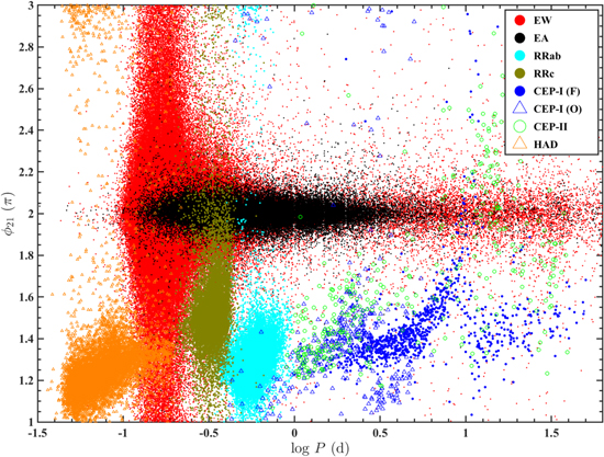
Figure 1. ϕ21 vs. logP diagram for all ZTF variables with characteristic LCs. From short to long periods, these include high-amplitude δ Scuti stars (HADs; orange), EW-type eclipsing binaries (red), RRc Lyrae (dark green), RRab Lyrae (cyan), EA-type eclipsing binaries (black), first-overtone classical Cepheids (blue triangles), fundamental-mode classical Cepheids (blue filled circles), and Type II Cepheids (green open circles).
Download figure:
Standard image High-resolution image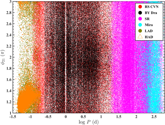
Figure 2. ϕ21 vs. logP diagram for all ZTF variables with noncharacteristic LCs. From short to long periods, these include low-amplitude δ Scuti stars (LADs; dark green), RS CVn (red), BY Dra stars (black), SRs (magenta), and Miras (cyan). Orange HADs are also shown, for comparison with the LADs.
Download figure:
Standard image High-resolution imageEclipsing binaries can be divided into EW, semidetached (EB), and detached (EA) types according to the degree by which they fill their Roche lobes. An accurate classification requires a detailed orbital analysis, which represents a major effort. Fortunately, we can also use well-established empirical relations related to their LCs. We refitted the LCs of our sample of eclipsing binaries using their full periods. The newly determined Fourier parameters a2 and a4 (similar to a1 and a2 pertaining to their half periods) and the difference between the primary and secondary minimum magnitudes  were obtained to perform the classification. Compared with EW-type eclipsing binaries, EA-type objects have a larger amplitude a4. To separate EW from EA types, we used the (a4, a2) diagram, similarly to Chen et al. (2018b).
We also adopted  (see Figure 4) as an additional boundary to identify eclipsing binaries that were not well separated based on the equations of Chen et al. (2018b). The main difference between semidetached and contact eclipsing binaries is the difference between both minima. Both components of contact eclipsing binary systems share a common envelope and, as a result, they have similar temperatures. However, semidetached eclipsing binaries usually exhibit larger Δmin because of the different temperatures of the two components. Δmin = 0.2 mag (corresponding to a 5% difference between the components' temperatures for an inclination of i = 90°) is usually adopted as the boundary between semidetached and contact eclipsing binaries. This criterion offers a rough classification of the two subtypes, and it is reliable for higher orbital inclinations (i > 70°) and good photometric quality. We did not try to classify and distinguish semidetached eclipsing binaries from other types of eclipsing binaries. Instead, we recorded the two-band minimum differences Δmin in our catalog to facilitate any further classification based on future DRs.
The main subtypes of Cepheids among our candidates are classical Cepheids pulsating in their fundamental and first-overtone modes and Type II Cepheids. Classical and Type II Cepheids cannot be separated cleanly only based on LC information. However, classical Cepheids are 2 or 3 mag brighter than Type II Cepheids. In addition, classical Cepheids are young and associated with the Milky Way's thin disk. Armed with these two additional classification criteria, both Cepheid types can be separated more easily. The fundamental and first-overtone classical Cepheids exhibit different LC shapes. First-overtone Cepheids usually have smaller amplitudes (Amp. < 0.4 mag) and a low amplitude ratio (R21 < 0.3). In Figures 3 and 4, we can see a clear boundary between fundamental (blue filled circles) and first-overtone (blue triangles) classical Cepheids (see also Soszynski et al. 2008). Just like for Cepheids, RRab and RRc Lyrae pulsating in their fundamental and first-overtone modes also exhibit a clear boundary.
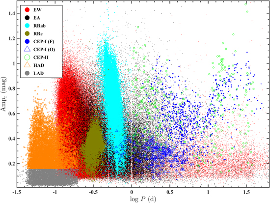
Figure 3. Ampr vs. logP diagram for all ZTF variables. Symbols are as in Figure 1. LADs have been added as gray filled circles.
Download figure:
Standard image High-resolution image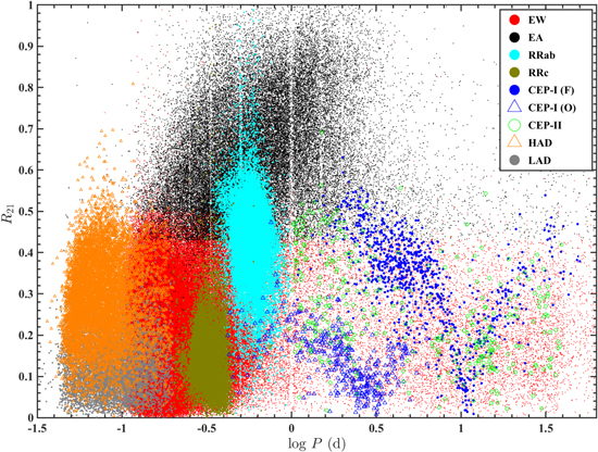
Figure 4. R21 vs. logP diagram for all ZTF variables. Symbols are as in Figure 3.
Download figure:
Standard image High-resolution image4.1. Luminosity Selection
Luminosity is the other important parameter one can use to classify variables. We present the period–luminosity diagram in Figure 5. Variables with Gaia parallax accuracy better than 20% are shown, except for the luminous variables, since most of the latter are distant and exceed our parallax constraint. Cepheids with <100% parallax uncertainty, Miras with <50% parallax uncertainty, and SRs with <50% parallax uncertainty are shown. Variables outside these ranges exhibit more scatter in their absolute magnitude distributions and a tail at faint magnitudes, which is the result of the Lutz–Kelker effect.

Figure 5. logP vs.  diagram for variables with better than 20% (all variables except giants), 50% (Miras and SRs), and 100% (Cepheids) Gaia parallax accuracy.
  are the absolute Weisenheit magnitudes estimated from a combination of g, r photometry and Gaia parallaxes. Symbols are as in Figure 4. Miras, SRs, and BY Dra variables have been added using blue plus signs and pink and green filled circles, respectively.
Download figure:
Standard image High-resolution imageδ Scuti stars, RRab and RRc Lyrae, and classical Cepheids that are located in the instability strip follow tight period–luminosity relations (PLRs). The scatter in their absolute magnitudes is mainly caused by parallax uncertainties. We adopted  to exclude dwarf contamination. Here,
  and
and  are the observed and predicted absolute magnitudes, respectively, and σDM is the error in the distance modulus, which has been propagated from the parallax uncertainty. The
  –P relations for these variables were calculated using objects with parallax uncertainties less than 10%. Since these PLRs were roughly determined and only used to exclude contamination, we do not report the corresponding coefficients here. For more accurate PLRs, we refer to individual papers discussed in Section 6.
In Figure 5, we find that both HADs and LADs follow similar PLRs, and their scatter seems smaller than that pertaining to the RR Lyrae and Cepheids. This smaller scatter is driven by the high number of nearby δ Scuti stars. Except for these variables, EW-type eclipsing binaries, Type II Cepheids, SRs, and Miras also follow PLRs characterized by moderate scatter. EW-type eclipsing binaries have been found to obey PLRs with 6%–7% accuracy in infrared bands (Chen et al. 2016a, 2018a). SRs and Miras are LPVs that obey different sequences in the period–luminosity diagram (Lebzelter et al. 2019). Without access to accurate parallaxes and well-determined periods, their sequences are rather unclear.
At the bottom of the the period–luminosity diagram, we find that BY Dra variables are vertically distributed in the range of  mag, and they are fainter than other variables. This BY Dra sequence is always clear in a parallax-limited sample, which means that this is a real distribution rather than one caused by selection effects associated with the limit imposed on the Gaia parallaxes. Since the absolute magnitude boundary for BY Dra variables is unknown, we adopted these rough luminosity cuts to classify BY Dra stars. The rotational periods of BY Dra variables range from 0.25 to 20 days, with a peak around a few days. RS CVn occupy the same distribution as eclipsing binaries. They are not shown in the diagram. The PLRs or luminosity ranges were determined for each variable type to help with our classification. For example, candidates 2 mag fainter than classical Cepheids have a low probability of being classical Cepheids.
For candidates in the overlap region in parameter space, such as RRc and EW-type eclipsing binaries, Cepheids and rotational variables, LADs, and EW-type eclipsing binaries, we performed a visual check of their LCs to assist with and confirm the classification process. We thus classified 781,602 periodic variables from our master sample of 2.1 million candidates. The remaining candidates were recorded as suspected variables. They will be better classified based on enhanced data from future ZTF DRs.
5. The Periodic Variables Catalog
The periodic variables catalog9
of ZTF DR2, containing 781,602 periodic variables, is included in Table 2. It contains the source ID, position (J2000 R.A. and decl.), period, mean magnitudes ( ,
,  ), number of detections, LC parameters, and type of variable star. The LC parameters include the amplitude, amplitude ratio R21, phase difference ϕ21, Heliocentric Julian Date (HJD) of the minimum T0, R2 of the LC fit, two-band minimum differences for eclipsing binaries, and the period's FAP. Candidates without a good classification are collected in a suspected variables catalog (Table 3). The single-exposure photometry catalog is available online, including the objects' source ID, R.A. (J2000), decl. (J2000), HJD, gmag, rmag, e_gmag, and e_rmag. Figure 6 shows the density distribution of these periodic variables in Galactic coordinates. This density distribution is similar to the distribution of the number of detections. 74% of the variables are located in the northern Galactic plane (
 ), where variables have thus far not been recorded systematically.
Table 2. ZTF Variables Catalog
| ID | R.A. (J2000) | Decl. (J2000) | Period | R21 |

|
T0 |

|

|
... | Ampg | Ampr | Type |
|---|---|---|---|---|---|---|---|---|---|---|---|---|
| (deg) | (deg) | (days) | HJD −2,400,000.5 | (mag) | (mag) | ... | (mag) | (mag) | ||||
| ZTF J000000.13+620605.8 | 0.00056 | 62.10163 | 1.9449979 | 0.198 | 5.189 | 58386.2629478 | 17.995 | 16.571 | ... | 0.113 | 0.078 | BYDra |
| ZTF J000000.14+721413.7 | 0.00061 | 72.23716 | 0.2991500 | 0.263 | 6.308 | 58388.2555794 | 19.613 | 18.804 | ... | 0.540 | 0.438 | EW |
| ZTF J000000.19+320847.2 | 0.00080 | 32.14645 | 0.2870590 | 0.010 | 8.024 | 58280.4780813 | 15.311 | 14.610 | ... | 0.219 | 0.197 | EW |
| ZTF J000000.26+311206.3 | 0.00109 | 31.20176 | 0.3622166 | 0.132 | 6.281 | 58283.4619944 | 16.350 | 15.844 | ... | 0.233 | 0.226 | EW |
| ZTF J000000.30+233400.5 | 0.00125 | 23.56682 | 0.2698738 | 0.193 | 6.302 | 58437.2686640 | 17.890 | 16.944 | ... | 0.373 | 0.352 | EW |
| ZTF J000000.30+711634.1 | 0.00125 | 71.27616 | 0.2685154 | 0.160 | 5.236 | 58657.4235171 | 19.144 | 17.875 | ... | 0.173 | 0.154 | EW |
| ZTF J000000.39+605148.8 | 0.00163 | 60.86358 | 0.5591434 | 0.424 | 6.322 | 58338.4702019 | 19.965 | 19.002 | ... | 0.797 | 0.841 | EW |
| ZTF J000000.51+583238.7 | 0.00215 | 58.54409 | 2.9797713 | 0.143 | 9.013 | 58663.4378649 | 16.586 | 15.368 | ... | 0.082 | 0.068 | BYDra |
| ZTF J000001.00+612832.8 | 0.00420 | 61.47580 | 0.3643510 | 0.285 | 6.400 | 58385.2702714 | 20.640 | 19.627 | ... | 0.970 | 0.681 | EW |
| ZTF J000001.37+561504.9 | 0.00571 | 56.25137 | 0.2557214 | 0.312 | 6.256 | 58471.1392038 | 19.416 | 18.559 | ... | 0.674 | 0.623 | EW |
| ZTF J000001.74+614940.9 | 0.00729 | 61.82803 | 1.0158276 | 0.370 | 6.366 | 58349.3156217 | 19.094 | 18.013 | ... | 0.289 | 0.228 | EW |
| ZTF J000001.75+594739.4 | 0.00732 | 59.79428 | 112.0533126 | 0.390 | 6.950 | 58320.7237689 | 18.676 | 17.393 | ... | 0.062 | 0.055 | SR |
| ZTF J000001.92+554800.7 | 0.00804 | 55.80020 | 112.3366840 | 0.209 | 5.763 | 58389.1259060 | 12.664 | 0.0 | ... | 0.114 | 0.0 | SR |
| ZTF J000002.02+540550.8 | 0.00844 | 54.09746 | 7.6299744 | 0.677 | 3.277 | 58472.1363770 | 18.176 | 17.187 | ... | 0.187 | 0.151 | RSCVN |
| ZTF J000002.20+480720.8 | 0.00918 | 48.12246 | 0.3810135 | 0.227 | 3.701 | 58282.4549819 | 17.196 | 16.037 | ... | 0.107 | 0.093 | BYDra |
| ZTF J000002.21+385226.4 | 0.00921 | 38.87401 | 0.4103992 | 0.168 | 6.512 | 58274.4798066 | 15.265 | 14.853 | ... | 0.209 | 0.211 | EW |
| ZTF J000002.27+331411.5 | 0.00947 | 33.23655 | 0.1161226 | 0.069 | 3.714 | 58367.3685172 | 18.781 | 17.726 | ... | 0.238 | 0.197 | RSCVN |
| ZTF J000002.28+592423.4 | 0.00954 | 59.40651 | 0.3286918 | 0.063 | 5.511 | 58314.4511431 | 20.860 | 19.268 | ... | 0.280 | 0.255 | EW |
| ZTF J000002.61+560944.8 | 0.01091 | 56.16245 | 0.2780012 | 0.095 | 5.197 | 58644.4715685 | 16.017 | 15.664 | ... | 0.074 | 0.074 | RSCVN |
| ZTF J000002.69+640614.8 | 0.01123 | 64.10413 | 0.4084968 | 0.250 | 6.617 | 58307.4094573 | 21.241 | 19.953 | ... | 0.471 | 0.440 | EW |
| ZTF J000002.99+611736.0 | 0.01246 | 61.29334 | 0.5534820 | 0.269 | 6.289 | 58431.2049383 | 17.362 | 16.649 | ... | 0.241 | 0.228 | EW |
| ZTF J000003.05+410045.6 | 0.01271 | 41.01267 | 0.2701826 | 0.236 | 6.311 | 58296.3618793 | 16.796 | 16.055 | ... | 0.365 | 0.354 | EW |
| ZTF J000003.10+722838.4 | 0.01292 | 72.47736 | 0.2000857 | 0.014 | 5.677 | 58364.3618372 | 17.146 | 16.473 | ... | 0.069 | 0.054 | RSCVN |
| ZTF J000003.13–022548.2 | 0.01306 | −2.43006 | 0.4936916 | 0.431 | 3.906 | 58456.1669642 | 17.510 | 17.347 | ... | 1.301 | 0.902 | RR |
| ZTF J000003.17+582138.3 | 0.01325 | 58.36065 | 331.9141625 | 0.334 | 6.273 | 58400.7947631 | 13.180 | 0.0 | ... | 0.073 | 0.0 | SR |
| ZTF J000003.23+543605.4 | 0.01347 | 54.60151 | 0.7863971 | 0.105 | 8.826 | 58389.2748730 | 17.639 | 16.527 | ... | 0.166 | 0.112 | BYDra |
| ZTF J000003.24+692214.2 | 0.01353 | 69.37062 | 0.3728018 | 0.169 | 6.048 | 58282.4524423 | 15.855 | 14.678 | ... | 0.398 | 0.359 | EW |
| ZTF J000003.33+550558.3 | 0.01390 | 55.09955 | 0.2513022 | 0.377 | 6.044 | 58646.4653817 | 20.761 | 19.701 | ... | 0.765 | 0.773 | EW |
| ZTF J000003.40+623837.5 | 0.01419 | 62.64377 | 0.2627338 | 0.288 | 6.245 | 58362.3199849 | 21.027 | 19.922 | ... | 0.573 | 0.605 | EW |
| ZTF J000003.74+393925.9 | 0.01559 | 39.65722 | 0.2394832 | 0.050 | 7.755 | 58325.4868272 | 17.943 | 16.731 | ... | 0.192 | 0.158 | EW |
| ZTF J000003.74+623637.4 | 0.01560 | 62.61040 | 0.3755206 | 0.344 | 6.383 | 58343.3639966 | 20.429 | 19.378 | ... | 0.653 | 0.652 | EW |
| ZTF J000003.76+532917.1 | 0.01568 | 53.48811 | 0.5921959 | 0.408 | 7.638 | 58352.3259739 | 16.446 | 15.747 | ... | 0.164 | 0.159 | BYDra |
| ZTF J000003.88+553759.9 | 0.01619 | 55.63331 | 0.2652778 | 0.341 | 6.266 | 58348.4098300 | 19.632 | 18.711 | ... | 0.747 | 0.661 | EW |
| ZTF J000003.88+673554.8 | 0.01620 | 67.59858 | 7.8057274 | 0.096 | 6.155 | 58386.3788529 | 20.419 | 18.262 | ... | 0.498 | 0.426 | EW |
| ZTF J000003.92+614456.1 | 0.01636 | 61.74894 | 0.3473332 | 0.272 | 6.092 | 58257.4187066 | 20.679 | 19.451 | ... | 0.521 | 0.511 | EW |
| ZTF J000003.96+182425.2 | 0.01654 | 18.40700 | 0.4851359 | 0.456 | 3.909 | 58295.4504510 | 15.268 | 15.096 | ... | 1.126 | 0.879 | RR |
| ZTF J000004.14+570616.8 | 0.01725 | 57.10468 | 246.2392553 | 0.319 | 3.591 | 58347.9920985 | 15.589 | 13.508 | ... | 1.600 | 1.459 | SR |
| ZTF J000004.34+554359.8 | 0.01809 | 55.73328 | 0.3470882 | 0.272 | 6.349 | 58274.4650397 | 19.871 | 19.026 | ... | 0.602 | 0.610 | EW |
| ZTF J000004.34+522031.5 | 0.01809 | 52.34209 | 4.0833915 | 0.189 | 7.602 | 58320.3673808 | 17.703 | 16.745 | ... | 0.087 | 0.095 | BYDra |
| ZTF J000004.34+510505.0 | 0.01810 | 51.08474 | 0.3332412 | 0.034 | 4.458 | 58635.4032937 | 17.188 | 16.681 | ... | 0.192 | 0.191 | EW |
| ZTF J000004.41+581846.9 | 0.01840 | 58.31303 | 0.4418413 | 0.126 | 3.603 | 58278.4683106 | 18.842 | 17.921 | ... | 0.110 | 0.088 | BYDra |
| ZTF J000004.49+514615.4 | 0.01871 | 51.77095 | 0.0918632 | 0.187 | 4.174 | 58428.2433174 | 17.392 | 17.104 | ... | 0.161 | 0.115 | DSCT |
| ZTF J000004.56+453022.7 | 0.01902 | 45.50633 | 6.6168334 | 0.084 | 6.243 | 58490.2445564 | 16.378 | 15.673 | ... | 0.047 | 0.052 | RSCVN |
| ZTF J000004.98+524230.9 | 0.02076 | 52.70860 | 7.1420745 | 0.359 | 6.024 | 58471.1790394 | 17.357 | 15.933 | ... | 0.080 | 0.072 | BYDra |
| ZTF J000005.00+555613.9 | 0.02087 | 55.93720 | 0.8834472 | 0.278 | 6.004 | 58332.3958118 | 18.238 | 16.738 | ... | 0.141 | 0.131 | EW |
| ZTF J000005.13+503833.5 | 0.02138 | 50.64264 | 6.8118535 | 0.046 | 4.986 | 58316.3336707 | 16.984 | 16.128 | ... | 0.125 | 0.072 | BYDra |
| ... | ... | ... | ... | ... | ... | ... | ... | ... | ... | ... | ... | ... |
Only a portion of this table is shown here to demonstrate its form and content. A machine-readable version of the full table is available.
Download table as: DataTypeset image
Table 3. ZTF Suspected Variables Catalog
| ID | R.A. (J2000) | Decl. (J2000) |

|

|
Periodg | Periodr | Ampg | Ampr | Numg | Numr | log (FAP)g |
|---|---|---|---|---|---|---|---|---|---|---|---|
| (deg) | (deg) | (mag) | (mag) | (days) | (days) | (mag) | (mag) | ||||
| ZTF J000000.06+583327.2 | 0.00026 | 58.55756 | 12.974 | 12.324 | 1.00157 | 0.05415 | 0.059 | 0.057 | 118 | 137 | −5.865 |
| ZTF J000000.09+632559.3 | 0.00041 | 63.43315 | 15.137 | 14.451 | 339.5882 | 344.55948 | 0.075 | 0.038 | 124 | 146 | −6.685 |
| ZTF J000000.14+552150.6 | 0.00060 | 55.36408 | 17.081 | 15.919 | 0.49772 | 0.09674 | 0.049 | 0.024 | 121 | 143 | −5.067 |
| ZTF J000000.15+540322.4 | 0.00066 | 54.05624 | 18.144 | 16.776 | 0.49768 | 0.10488 | 0.087 | 0.023 | 122 | 144 | −5.566 |
| ZTF J000000.16+621059.7 | 0.00069 | 62.18326 | 16.454 | 15.585 | 0.4979 | 0.08946 | 0.046 | 0.018 | 125 | 146 | −5.494 |
| ZTF J000000.17+592103.3 | 0.00073 | 59.35093 | 17.342 | 16.391 | 0.99392 | 0.13364 | 0.055 | 0.026 | 124 | 147 | −4.545 |
| ZTF J000000.25+605628.0 | 0.00108 | 60.94112 | 17.745 | 15.993 | 0.99385 | 0.44865 | 0.127 | 0.019 | 125 | 146 | −3.811 |
| ZTF J000000.27+665503.0 | 0.00116 | 66.91750 | 16.711 | 15.505 | 251.12632 | 0.05878 | 0.069 | 0.021 | 169 | 186 | −6.459 |
| ZTF J000000.28+583810.1 | 0.00119 | 58.63614 | 15.121 | 14.359 | 295.46337 | 0.33318 | 0.068 | 0.059 | 118 | 138 | −5.534 |
Only a portion of this table is shown here to demonstrate its form and content. A machine-readable version of the full table is available.
Download table as: DataTypeset image

Figure 6. Distribution map (in Galactic coordinates) of the 781,602 periodic variables classified in ZTF DR2.
Download figure:
Standard image High-resolution image5.1. New Variables
We cross-matched our variables catalog with several other large variable catalogs to check the accuracy of our classification and of the derived periods, as well as the completeness of our catalog. The reference catalogs include the ASAS-SN Catalog of Variable Stars in the Northern Hemisphere, the ASAS-SN Catalog of Variable Stars with a reclassification of 412,000 known variables, the ATLAS catalog of variables, the WISE catalog of periodic variable stars, the Catalina catalog of periodic variable stars, the Gaia catalog of RR Lyrae and Cepheids, the OGLE variables catalog, and other variables collected in the General Catalogue of Variable Stars (GCVS). We assembled these catalogs and then used an angular radius of 2'' to match the nearest known variables to our ZTF variables. Almost all objects were detected within 1'', which means that the recent variable surveys all have good positional accuracy. In addition, a 1'' matching radius can significantly reduce sample confusion, which is a potentially serious problem in dense fields. A total of 621,702 of the 781,602 variables in the ZTF database are newly detected variables. The total number and the number of newly detected variables of each type are listed in Table 4. The new detection rate of these variables is high, ranging from 10% for RRab Lyrae to more than 90% for δ Scuti and BY Dra variables. This high new detection rate is the result not only of the database's high photometric accuracy (∼0.02 mag accuracy down to r = 18 mag) and the faint limiting magnitude of the ZTF database (about 1.5 mag deeper than ATLAS in the corresponding r band) but also of the improvements made in our method of variable-star identification and classification. The relatively low new detection rate of RRab Lyrae is explained easily, because they were already well covered by the Catalina survey and Gaia DR2. However, both the purity and the period accuracy of the RRab Lyrae are significantly improved in our ZTF catalog.
Table 4. All and Newly Detected ZTF Variables
| Type | Total | New (Fraction) |
|---|---|---|
| Cep-I | 1262 | 565 (44.8%) |
| Cep-II | 358 | 154 (43.0%) |
| RRab | 32,518 | 3034 (9.3%) |
| RRc | 13,875 | 2178 (15.7%) |
| δ Scuti | 16,709 | 15,396 (92.1%) |
| EW | 36,9707 | 306,375 (82.9%) |
| EA | 49,943 | 40,201 (80.5%) |
| Mira | 11,879 | 4,997 (42.1%) |
| SR | 119,261 | 97,737 (82.0%) |
| RS CVn | 81,393 | 70,957 (87.2%) |
| BY Dra | 84,697 | 80,108 (94.6%) |
| Total number | 781,602 | 621,702 (79.5%) |
Download table as: ASCIITypeset image
5.2. Classification Accuracy
The classification accuracy pertaining to each type of variable was tested by comparison with the four variable-star catalogs; see Table 5. The coincidence rates range from 95% to 99%, with any disagreement usually found at the faint end for each catalog. In addition, different sampling strategies may also result in somewhat inconsistent classifications. We note that a few (sub)types have relatively low coincidence rates of around 80%. This means that the standard of classification for these variables is not well established. Among the four catalogs we compared our results with, the ASAS-SN catalog has the best classification accuracy overall.
Table 5. Variable Purity Comparison between ZTF and Other Catalogs
| Type | ATLAS | ASAS-SN | Catalina | WISE | Total Sample |
|---|---|---|---|---|---|
| RRab | 99.8% | 98.6% | 98.8% | 96.2% | 99.0% |
| RRc | 89.0% | 90.4% | 93.9% | 91.2% | |
| EW | 95.1% (99.8%)a | 95.1% (97.1%) | 97.1% (97.7%) | 96.3% (98.4%) | 95.6% (98.7%) |
| EA | 82.0% (99.8%) | 93.6% (96.0%) | 70.5% (98.3%) | 95.6% (98.5%) | 84.3% (99.2%) |
| Cep-I | 98.5% | 84.1% | 96.1% | 91.7% | |
| Cep-II | 96.9% | 82.8% | 94.5% | 88.1% | 90.1% |
| SR | 97.7% | 98.0% | 97.9% | ||
| Mira | 88.5% | 53.3% | 69.3% | ||
| δ Scuti | 83.5% | 94.6% | 85.5% | 87.6% | |
| RS CVn | 75.2% | 75.2% | |||
| BY Dra | 93.7% | 93.7% |
Note.
aThe purities in brackets only account for contamination by nonbinary variables.Download table as: ASCIITypeset image
In our catalog, RRab Lyrae have the best classification standard. Their purity is around 99%. The main contaminants are unsolved RRc Lyrae and EW-type eclipsing binaries. RRc Lyrae exhibit a purity of 91%. Their more symmetric LCs can easily mask them as EW-type eclipsing binaries. The purity of the eclipsing binaries is not as high as that of the RRab Lyrae. This is because of the difficulty in unequivocal classifications among the three binary subtypes. For lower LC amplitudes the classification becomes rather difficult. In this paper, we classify all eclipsing binaries into EW and EA types. Contamination by nonbinaries is only 1%. This means that our separation of binaries from pulsators is efficient. EW-type eclipsing binaries have a purity of 96%; their main contaminants are EA-type eclipsing binaries. EA-type eclipsing binaries have a coincidence rate of 84%.
The coincidence rate of classical Cepheids is around 92%, based on a comparison of ∼200 known Cepheids. The percentage of disagreement for Type II Cepheids is around 10%. LPV purity is around 98%. Here, the main misclassification occurs between SRs and Miras, even though all reference catalogs adopted a similar boundary, Amp. = 2.0 mag. These different classifications can be explained by the different limiting magnitudes pertaining to the reference catalogs: a shallow limiting magnitude will lead to underestimated Mira amplitudes. For example, the ASAS-SN catalog has a limiting magnitude of 17, so that for Miras fainter than 15 mag, the amplitude determined is likely less than 2 mag. These Miras will hence be classified as SRs, and as a result, about 46% of matched Miras are mistaken for SRs in the ASAS-SN catalog. In turn, 99.2% of ASAS-SN Miras are correctly classified in our catalog. Toward the faint magnitude limit of ZTF, this type of misclassification also occurs. In our catalog, 1694 SRs with mg,r > 19 mag and Ampr > 1.0 (Ampg > 1.2) mag run the risk of misclassification.
The short-period δ Scuti variables have a purity of 88%. However, δ Scuti stars are not well classified in previously published catalogs. In our catalog, the purity of HADS is as high as those of RR Lyrae and eclipsing binaries, while the LADS purity is relatively lower. As regards rotational stars, the purity of BY Dra (93.7%) is high since they were strictly selected based on their Gaia parallaxes. However, without a luminosity criterion, it is not easy to separate RS CVn and eclipsing binaries with poor-quality photometry. To obtain a cleaner sample of eclipsing binaries, many eclipsing binaries with relatively poor-quality LCs have been classified as RS CVn, which leads to a systematically lower purity level of RS CVn (75.2%). Given that we have double-checked the LCs of all variables where we noticed disagreement with other catalogs, our classification is more reliable for most of these objects. This is reasonable, since ZTF is deeper, has better-quality photometry, and has been obtained in two passbands. However, toward the faint end of the ZTF, the ZTF sample purity will also decrease.
5.3. Period Accuracy
ZTF DR2 covers a time span of 470 days, so the periods in our catalog are most accurate for P ≲ 100 days. This limitation causes problems for the periods of SRs and Miras. Period problems pertaining to short-period variables are usually caused by the limited sampling cadence, e.g., a daily cadence is a major problem for ground-based time-domain surveys. Except for the WISE catalog, the other three previously published catalogs and the ZTF catalog are all affected by this problem. This period problem is not easily eliminated by increasing the sampling using the same cadence, but it can be reduced based on multipassband information and information about the physical properties of the variables. Figure 7 shows a comparison of the periods determined from the g and r LCs. One of the two periods is the real period (Pr), while the other is the aliased period (Pa). Both periods are found to mainly follow three relations:  (corresponding to the red dotted, dashed, and solid lines in Figure 7, respectively). We can justify which period is more reliable, e.g., the bright variables are usually LPVs (
 mag), or variables with ϕ21 < 4 are likely associated with RRab rather than RRc periods. However, for eclipsing binaries and δ Scuti stars, there is no significant feature to validate the real period. For example, assuming that δ Scuti stars have real and aliased periods of 0.08 and 0.074 days, respectively, it is hard to justify which period is real, even with access to their luminosities and ϕ21 phases. Therefore, we visually compared the folded LCs pertaining to the two periods individually for those variables. This process can determine the correct period for most variables if the LC quality is good.

Figure 7. Comparison of periods determined from the g- and r-band LCs. The red lines are the predicted relations between real and aliased periods.
Download figure:
Standard image High-resolution imageOur comparison of the four catalogs shows that our period accuracy is as high as 99%, except for LPVs and δ Scuti stars. The inconsistency rates for RRab, RRc, EW-type eclipsing binaries, and classical Cepheids range from 0% to 2% (Table 6). This is a common accuracy for large variable-star catalogs. The inconsistency rate of δ Scuti stars is a little higher, since their periods are much shorter than the sampling cadence. Complementary short-cadence observations can resolve this aliased period problem. The full- versus half-period problem occurred for a few EA-type eclipsing binaries with insignificant secondary eclipses. If we do not consider the full- versus half-period problem, the period accuracy of EA-type eclipsing binaries is as high as those for other short-period variables. We have visually checked the LCs of EA-type eclipsing binaries to ensure that they all show the full periods. As to LPVs, around 11% of Miras and 32% of SRs have period differences larger than 20% by comparison with the ASAS-SN and Catalina catalogs. The precision of Mira periods is limited by the observational time span. SRs usually contain several short- and long-term periods, so the low inconsistency derived here is not surprising. The accuracy of the LPV periods will be refined with the availability of future DRs.
Table 6. Period Comparison between ZTF and Other Catalogs
| Type | ATLAS | ASAS-SN | Catalina | WISE | Total Sample |
|---|---|---|---|---|---|
| RRab | 99.7% | 99.7% | 98.0% | 99.6% | 99.6% |
| RRc | 98.9% | 98.4% | 97.8% | 98.3% | |
| EW | 99.8% | 98.6% | 95.3% | 99.9% | 98.7% |
| EA | 92.9% (98.7%)a | 93.8% (99.4%) | 95.1% (98.1%) | 93.1% (99.7%) | 93.2% (98.9%) |
| Cep-I | 100% | 97.9% | 100% | 99.2% | |
| SR | 68.3% | 93.5% | 68.4% | ||
| Mira | 88.2% | 94.6% | 88.7% | ||
| δ Scuti | 98.8% | 94.8% | 91.5% | 96.6% |
Note.
aThe values in brackets do not take into account the full- versus half-period problem.Download table as: ASCIITypeset image
5.4. Completeness
We estimate the completeness of our catalog by comparison with previously published catalogs based on known variables in the ZTF magnitude range deemed reliable (r > 12.5 mag), as well as its spatial coverage (decl. > −13°). The completeness for the full sample is 71.1%. Since sampling of the ZTF is not homogeneous across the entire northern sky, the completeness varies with spatial position (see Figure 6). For regions at high declinations (decl. > 40°), the completeness can be as high as 76%. Some 24% of our variables are not classified because of insufficient sampling. The ZTF DR2 contains ∼150 detections for each object, a smaller number than the equivalent numbers of detections in the ASAS-SN and Catalina catalogs. As the declination decreases, the completeness gradually decreases to 50%. For different magnitude ranges, the completeness is always around 71.1%, which means that the completeness is not affected by the objects' apparent magnitudes or photometric uncertainties. With future DRs, ZTF will be able to detect and classify more than 1 million periodic variables in the northern sky, assuming current completeness levels. Gaia may be able to help classify 3 million periodic variables across the full sky, considering their enhanced density in the Galactic bulge and the Magellanic Clouds in the southern sky.
Except for spatial sampling, time sampling issues may also cause incompleteness. Since our catalog only covers a time span of 470 days, its completeness for LPVs is not as high as that for short-period variables. We compare the LPVs in the ASAS-SN catalog with our sample to estimate their completeness, since ASAS-SN covers both a longer time span and a larger number of LPVs. Globally, 42% of LPVs across the entire sky were rediscovered in our catalog. This fraction is some 30% lower than that for our full sample of variables.
5.5. Cepheids and RR Lyrae
In addition to our comparisons with the four variables catalogs, we also evaluated the periods and completeness levels of the Cepheids and RR Lyrae in our catalog by comparison with the OGLE and Gaia catalogs, both of which have similar depths to ZTF. OGLE IV recently released their variables catalog of Cepheids and RR Lyrae in the Galactic disk (Skowron et al. 2019a; Soszyński et al. 2019). Although the overlap region between OGLE and ZTF is limited, a comparison is still feasible. Gaia DR2 contains about 140,000 RR Lyrae across the full sky, as well as 500 classical Cepheids in the Milky Way.
As for the classical Cepheids, we compared our catalog with the 2682 high-probability Cepheids collected by the OGLE team (Pietrukowicz et al. 2013; Udalski et al. 2018). The number of objects in common is 691, and the completeness of our ZTF Cepheids is 63.3% given that 1092 of the full sample of Cepheids are located in the ZTF's detection region. This relatively low completeness level compared with the global completeness of our variables catalog suggests that the completeness of variable types with intermediate periods is lower than that of short-period variables. Only 2 of the 691 confirmed objects have inconsistent periods. Having double-checked these periods, we conclude that our periods are more reliable.
OGLE IV contains 10,000 RR Lyrae in the Galactic disk, and two of their fields overlap with the field covered by the ZTF catalog. We found that 1327 of the 1854 (71.6%) OGLE RR Lyrae in these two fields have been rediscovered in our catalog; 99.5% of these 1327 RR Lyrae have consistent periods. Both the period accuracy and completeness are in agreement with the equivalent values pertaining to the full catalog. For RR Lyrae contained in Gaia DR2, 39,301 are located in the ZTF's detection region. Some 80.1% (31483) of Gaia RR Lyrae have been rediscovered in our catalog. This completeness level is 9% higher than the catalog's global completeness of 71.1%, which is mainly driven by the incompleteness levels characteristic of Gaia RR Lyrae. About 400 of the Gaia RR Lyrae are contaminated by EW-type eclipsing binaries and δ Scuti stars.
6. Discussion
In this section, we discuss for each type of variable their LCs, their PLRs, and their applications as potential distance tracers.
6.1. Cepheids
Classical Cepheids are the most important primary distance tracers. They are widely used for estimating distances to galaxies in the Local Volume and measuring the near-field Hubble constant (Riess et al. 2019). Because of their young age, classical Cepheids are also the best stellar tracer of the Galactic disk. Compared with extragalactic Cepheids, Cepheids in our Milky Way are rare. Before 2018, only around 1000 Milky Way Cepheids had been detected (Pojmanski et al. 2005; Berdnikov 2008). These Cepheids were distributed within 3 kpc of the Sun and showed few features of our Milky Way's structure. In 2018, several times the number of previously known classical Cepheids were found. The WISE catalog of variables listed about 1000 Cepheids that were homogeneously distributed across the Galactic plane, except for the Galactic center direction. OGLE detected another 1000 Cepheids in the southern disk. ALTAS, ASAS-SN, and Gaia also detected several hundred Cepheids.
This rapid increase in the number of Cepheids motivated studies of the Milky Way's disk. Samples of 1339–2500 carefully selected disk Cepheids revealed the first intuitive 3D map of our Galaxy's stellar disk (Chen et al. 2019; Skowron et al. 2019b). The outer disk was found to be warped, and the warp is now known to be precessing (Chen et al. 2019). Recently, 640 new Cepheids in the southern disk affected by heavy extinction were discovered by the VVV survey (Dékány et al. 2019). In our ZTF catalog, we found an additional 565 new classical Cepheids, thus further enlarging the sample in the northern warp and around the edge of the disk. Figure 8 shows the distribution of 3300 well-determined disk classical Cepheids (satisfying the Gaia parallax and LC criteria), which agree with the warp model of Chen et al. (2019) to within 1σ–2σ. This new sample of Cepheids is sufficient to trace the detailed morphology of the disk beyond Galactocentric distances of 15 kpc. In the (X, Y) plane, the Cepheid distribution is not homogeneous, but it shows bubble and filament features. A significant bubble is found at a distance of about 6 kpc from the Sun in the Galactic anticenter direction. With a detailed study of these features, we could potentially infer the dynamical evolution history of the Galactic disk.
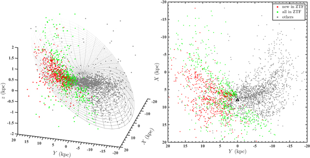
Figure 8. Milky Way disk in 3D (left) based on ∼3300 Cepheids and their projection onto the (X,Y) plane (right). Red: new Cepheids in the ZTF catalog; green: other Cepheids in ZTF catalog; gray: Cepheids from OGLE, WISE, ATLAS, ASAS-SN, and other catalogs. The grid in the left panel represents the warp model of Chen et al. (2019). The triangle in the right panel denotes the position of our Sun.
Download figure:
Standard image High-resolution imageIn the future, new Cepheids are expected to be found in the Galactic center direction (Matsunaga et al. 2011; Dékány et al. 2015). In addition, low-amplitude or long-period Cepheids will be classified once more accurate parallaxes become available. Our larger sample of Cepheids will also be helpful in determining the zero points and slopes of their PLRs (Breuval et al. 2019), particularly of infrared PLRs (Chen et al. 2017; Wang et al. 2018). In addition to Cepheids in the Milky Way, we also found 21 Cepheids (one new Cepheid) associated with M31 (Kodric et al. 2018), one Cepheid in M33 (Hartman et al. 2006), and one in IC 1613 (Udalski et al. 2001). ZTF DR2 contains only about 50 detections in the M31 direction. With increased sampling in future DRs, several hundred Cepheids will likely be found in M31.
Cepheid LCs in g and r are shown in Figure 9. From their LCs, the majority of classical Cepheids can be divided into fundamental-mode (Figure 9(a)) and first-overtone Cepheids (Figure 9(b)). First-overtone Cepheids have lower amplitudes and shorter periods than the corresponding fundamental-mode Cepheids. At a given period, first-overtone Cepheids have slightly brighter luminosities. This magnitude difference is around 0.5 mag in the LMC (Inno et al. 2016), Small Magellanic Cloud (SMC; Ripepi et al. 2017), and M31 (Kodric et al. 2018), while the situation in the Milky Way is less clear (Ripepi et al. 2019). With an increasing number of first-overtone Cepheids and better parallaxes, the PLRs of Milky Way Cepheids will be better constrained.

Figure 9. Example LCs for (a) fundamental-mode classical Cepheids, (b) first-overtone classical Cepheids, and (c) Type II Cepheids. The blue filled circles and red plus signs are LCs in the g and r bands, respectively. From top to bottom, phase differences ϕ21 increase. The mean magnitudes are fixed at 0.6i + 0.2, 0.3i, and 0.8i (i = 0, 1, ..., 9) in the g band and 0.6i, 0.3i, and 0.8i in the r band, for fundamental-mode classical Cepheids, first-overtone classical Cepheids, and Type II Cepheids, respectively.
Download figure:
Standard image High-resolution imageCompared with classical Cepheids, the LC shapes of Type II Cepheids are more highly variable (Figure 9(c)). Type II Cepheids are older, fainter, and follow PLRs characterized by a somewhat larger scatter (Bhardwaj et al. 2017; Groenewegen & Jurkovic 2017). Type II Cepheids are mostly located away from the disk and associated with the Galactic bulge and halo. As distance indicators, Type II Cepheids can be used to study the structure of the bulge (Braga et al. 2018a) and measure the distances to globular clusters and dwarf galaxies. We found 154 new Type II Cepheids, which represents a significant increase and will be useful to anchor their PLRs and explore old Galactic structures.
6.2. RR Lyrae
RR Lyrae are the most numerous distance indicators in old environments. Their PLRs or PL–metallicity relations can be as accurate as those for the classical Cepheids (Catelan 2009, and references therein). In the Milky Way halo, RR Lyrae are used to trace dwarf galaxies and distant substructures (Drake et al. 2013; Sesar et al. 2017; Medina et al. 2018; Erkal et al. 2019; Martínez-Vázquez et al. 2019). RR Lyrae can be used to reveal structures out to distances of some 120 kpc. Better identification of RR Lyrae in the Dark Energy Survey can help to reach distances greater than 200 kpc (Stringer et al. 2019). RR Lyrae at moderate distances are usually used to determine accurate distances to globular clusters (Braga et al. 2018b; Bono et al. 2019; Palma et al. 2019). With a more complete sample, RR Lyrae are perhaps the best tracers to trace the Milky Way halo's shape (Iorio et al. 2018; Iorio & Belokurov 2019). In the Galactic inner regions, featuring numerous RR Lyrae, the shape of the bulge can also be constrained (Pietrukowicz et al. 2015; Gran et al. 2016). In the ZTF catalog, we detected more than 5000 new RR Lyrae out to distances of 125 kpc. We detected several RR Lyrae associated with the Draco dwarf galaxy at a distance of around 76 kpc (Bonanos et al. 2004). Unlike previous RR Lyrae samples, the new sample may reveal unknown structures at low Galactic latitudes ( ).
).
Studies of the physical properties of RR Lyrae will also benefit from large and complete samples. In recent years, many metal-rich RR Lyrae have been found (Chadid et al. 2017; Sneden et al. 2018), which challenge the traditional theory explaining these metal-poor and old variables. Both the WISE and ZTF catalogs focus on the Galactic disk; RR Lyrae in the disk are, with high probability, metal-rich. With LAMOST or SDSS-SEGUE spectra, the physical properties of a large sample of RR Lyrae can be investigated. In Figure 3, the distribution of RR Lyrae in the period–amplitude diagram is more scattered than dichotomous, which suggests that the well-known Oosterhoff dichotomy problem of RR Lyrae may just be due to a lack of intermediate-metallicity RR Lyrae (Fabrizio et al. 2019).
Similarly to classical Cepheids, most RR Lyrae can be divided into fundamental-mode (RRab) and first-overtone pulsators (RRc). Example LCs of RRab and RRc Lyrae are shown in Figure 10. The amplitudes of RRab Lyrae are larger, decreasing as the LCs become symmetric (from top to bottom in the left panel of Figure 10). This trend is the result of the period–amplitude relation and is only significant for RRab LCs. The PLRs or PL–metallicity relations of Milky Way RRab Lyrae can be studied with Gaia DR2 parallaxes (Muraveva et al. 2018; Layden et al. 2019; Neeley et al. 2019). The accuracy of these PLRs is mainly limited by parallax uncertainties. RRc Lyrae also follow PLRs, which are about 0.5 mag brighter than for RRab Lyrae at a given period. In Figure 5, RRc Lyrae seem to exhibit more scatter in their luminosities than RRab Lyrae. If we can better constrain the luminosities of RRc Lyrae, they may be potentially viable distance tracers. A number of RRab and RRc Lyrae exhibit multiple periods, and about one-third of the RRab Lyrae show period modulation. These special RR Lyrae will be analyzed with enhanced data from future DRs.

Figure 10. Example LCs for (a) RRab and (b) RRc Lyrae. The blue filled circles and red plus signs are LCs in the g and r bands, respectively. From top to bottom, phase differences ϕ21 decrease.
Download figure:
Standard image High-resolution image6.3. Eclipsing Binaries
The three types of eclipsing binaries are distinguished by their evolutionary stage. From EA- to EW-type eclipsing binaries, the period distribution gradually shifts to shorter periods. Statistically, EW-type eclipsing binaries tend to be older, with a peak in their age distribution around 4 Gyr. EA-type eclipsing binaries are young, with a peak age around 1 Gyr. The basic evolution of eclipsing binaries has recently become clear. Nuclear evolution and angular momentum loss are the main mechanisms (Hilditch et al. 1988; Nelson & Eggleton 2001; Yakut & Eggleton 2005; Stepien 2006; Jiang 2020). Both mechanisms run in parallel. Driven by angular momentum loss, the period decreases and both components become closer. When one component evolves to or away from the terminal main sequence, its radius increases. Until one component fills its Roche lobe, an EA-type eclipsing binary evolves to become an EB-type eclipsing binary. Then, with material and energy transferring from the primary to the secondary component, combined with possible mass reversal, the secondary component also fills its Roche lobe. The resulting system is an EW-type eclipsing binary. In Figure 1, the significant cutoff period of EW-type eclipsing binaries around 0.19 days is driven by the nuclear evolution timescale. The progenitor of the primary component of this 0.19-day EW-type eclipsing binary is a low-mass star with a nuclear evolution timescale very close to the age of the Galaxy.
Since their binary fraction is higher, eclipsing binaries account for a large proportion of variables in magnitude-limited samples. The fraction of EW-type eclipsing binaries was estimated at around 0.1% in the field (Rucinski 2006). It could be as high as 0.4% in a ∼4 Gyr environment (Chen et al. 2016b). This fraction does not correct for the low-inclination problem and only counts EW-type eclipsing binaries seen at higher inclinations (i > 40°–60°). In our catalog, the fraction of EW-type eclipsing binaries identified is 0.07%, which is a lower limit. If we consider the number of missing EW-type eclipsing binaries owing to insufficient sampling (see Section 5.4), that fraction can be as high as 0.1%.
Detached eclipsing binaries evolve on timescales as long as or even longer than those of EW-type eclipsing binaries. However, depending on the spatial separation and radius ratio of both components, we can only observe eclipses of detached eclipsing binaries with i ∼ = 90°. Consequently, the fraction of EA-type eclipsing binaries is lower than that of EW types. EB-type eclipsing binaries have the shortest evolution timescale and account for the lowest fraction among the three types of eclipsing binaries.
Figure 11 shows LCs of eclipsing binaries. Their shapes and amplitudes in both bands are almost the same and differ from those of pulsating stars. In the left panel, we can identify when the eclipses start in the LCs of EA-type eclipsing binaries. In the right panel, the eclipse onset in EW(EB)-type eclipsing binary LCs is hard to identify. In the period range of 0.25–0.56 days, EW-type eclipsing binaries follow tight infrared PLRs (Chen et al. 2018a) and can be potential distance indicators. The viability of these PLRs has been validated by eclipsing binaries from the ASAS-SN catalog (Jayasinghe et al. 2020c).
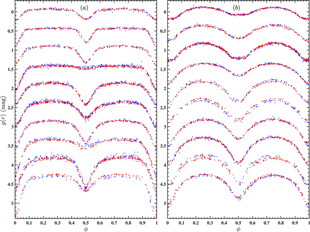
Figure 11. Example LCs for (a) EA- and (b) EW-type eclipsing binaries. The blue filled circles and red plus signs are LCs in the g and r bands, respectively. From top to bottom, the variation amplitudes increase.
Download figure:
Standard image High-resolution imageIn Figure 5, about 90,000 EW-type eclipsing binaries with <20% Gaia parallax uncertainties are found to also follow a PLR. In theory, the PLR of EW-type eclipsing binaries is driven by both Roche lobe theory and the mass–luminosity relation. Based on this PLR and a sample of several 100,000 EW-type eclipsing binaries, a better study of the detailed structure of the Milky Way will be possible. Except for distance determination, EW-type eclipsing binaries can also provide age information based on their periods. In addition, kinematic properties derived from Gaia data can provide constraints on the binaries' ages (Hwang & Zakamska 2020). We expect that the eight-dimensional parameter space pertaining to EW-type eclipsing binaries can be established and used to constrain the Milky Way's evolution. Without strict constraints on the secondary components, the PLR of EB-type eclipsing binaries exhibits more significant scatter. Less evolved, EA-type eclipsing binaries are the best objects to obtain absolute parameters from the orbital equations. By analyzing both their LCs and radial velocity curves, late-type EA-type eclipsing binaries can yield distances with 1% accuracy (Pietrzyński et al. 2019).
6.4. SRs and Miras
SRs and Miras are most likely red giants, red supergiants, or AGB stars exhibiting long-period–luminosity variations. They are important distance tracers in the context of the cosmological distance scale since they are brighter than classical Cepheids in infrared bands. However, LPVs follow multisequence PLRs, and each PLR sequence exhibits larger scatter (Lebzelter et al. 2019) than the classical Cepheid PLRs. To become a reliable distance indicator, LPV properties must be studied in more detail, particularly in the Milky Way and M31. The PLRs of red supergiants belonging to the LMC, SMC, M31, and M33 have been well studied, and their 1σ accuracy is 10%–15% in infrared bands (Yang & Jiang 2011, 2012; Ren et al. 2019). However, in the Milky Way, the number of red supergiants with reliable distances is too small to establish reliable PLRs (Chatys et al. 2019).
Oxygen-rich Miras also follow tight PLRs. In infrared bands, the 1σ scatter about their PLRs is around 10% (Yuan et al. 2017, 2018). Compared with red supergiants, Miras are 0–4 mag fainter but several times more numerous. All of these LPVs are potential tracers to measure the Hubble parameter (Huang et al. 2020). In the Milky Way, LPVs are young and intermediate-age structure tracers, complementary to Cepheids and RR Lyrae. Similarly to eclipsing binaries, the ages of each LPV subtype can be inferred from their periods (Mowlavi et al. 2018). As such, LPVs are also tracers that can constrain the evolution history of our Galaxy.
LCs of SRs and Miras are shown in the left and right panels of Figure 12, respectively. In the ZTF, several Miras are found with r-band amplitudes exceeding 6 mag. Since the total time span of the ZTF DR2 is 470 days, many Miras only have LCs available for at most one period. We detected about 130,000 LPVs, with the majority belonging to our Galaxy or to nearby dwarf galaxies. To better understand the physics of these LPVs, we also show them in color–magnitude and color–color diagrams (Figures 13(a), (b)). WISE W1, W1 − W2, and W2 − W3 magnitudes with good photometric signal-to-noise ratios (S/NW1 > 5, S/NW2 > 5, S/NW3 > 10) and quality were adopted to indicate LPV magnitudes and colors. This choice reduces the effects of the significant extinction in the Galactic plane. By comparison with massive stars in the LMC in color–absolute magnitude space (Yang et al. 2018), we find that SRs (blue filled circles in Figure 13) are composed of red giants, red supergiants, oxygen- and carbon-rich AGB stars, and extremely carbon-rich AGB stars. Miras (red filled circles) contain a few oxygen-rich, a few extremely carbon-rich, and many carbon-rich AGB stars.
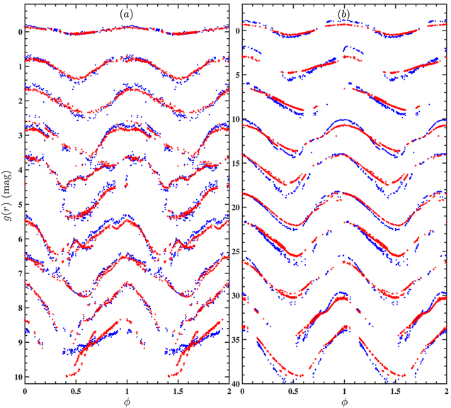
Figure 12. Example LCs for (a) SRs and (b) Miras. The blue filled circles and red plus signs are LCs in the g and r bands, respectively. From top to bottom, the variation amplitudes increase. The mean magnitudes are fixed at 1.0i and 4.0i (i = 0, 1, ..., 9) in the g and r bands, for SRs and Miras, respectively.
Download figure:
Standard image High-resolution image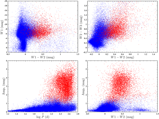
Figure 13. LPVs in the ZTF catalog. (a) Color–absolute magnitude diagram. (b) Color–color diagram. (c) Period–amplitude diagram. (d) Color–amplitude diagram. SRs and Miras are shown as red and blue filled circles, respectively.
Download figure:
Standard image High-resolution imageAGB populations are characterized by an absolute magnitude of about −8 mag in the mid-infrared, and the bright end of the red supergiant population is around −12 mag. Therefore, data points with magnitudes brighter than −12 mag in the left panel ( ) or brighter than −9 mag in the right panel (W1 − W2 > 0) are stars that may have larger parallax uncertainties. In Figure 13(c), the amplitudes grow monotonously as the periods increase. In particular, some sequences are found in the SR distribution, referred to as the A, B, and C' (third-, second-, and first-overtone) sequences (Trabucchi et al. 2017). Miras and some SRs form sequence C, which is the location of high-amplitude fundamental pulsators. In Figure 13(d), SRs and Miras are separated by a boundary, with Miras being high amplitude and red. The detailed subtype classification of these LPVs is not further discussed in this paper, as it requires access to better periods and parallaxes.
6.5. δ Scuti Stars
Among the variables in the ZTF, δ Scuti stars have the shortest periods. δ Scuti stars are main-sequence pulsators located in the instability strip, so they follow a PLR similar to RR Lyrae and Cepheids. Different from RR Lyrae and Cepheids, a fraction of δ Scuti stars is thought to exhibit multiple periods. The PLRs of δ Scuti stars are not well studied, even for HADs, because of their fainter magnitudes and limited sampling in the past. In the LMC, the magnitude range of δ Scuti stars ranges from 20 to 22 mag in the R band (Garg et al. 2010), which is close to the limiting magnitude of many time-domain surveys. PLRs of δ Scuti stars are therefore best studied in the Milky Way. Ziaali et al. (2019) tried to establish a V-band PLR based on 1100 δ Scuti stars in the Kepler field with good Gaia DR2 parallaxes; however, their PLR is not as tight as the equivalent PLRs pertaining to other tracers. Recently, Jayasinghe et al. (2020b) derived multiband PLRs for fundamental and overtone pulsators, based on ∼8400 δ Scuti stars from ASAS-SN, and found a 1σ scatter around 10%.
Our ZTF sample is several times larger and more homogeneously distributed across the northern sky, which paves the way to improve the δ Scuti PLRs. In Figure 5, we show that the Wesenheit PLR of δ Scuti stars is tight, with few outliers. A simple estimation shows that the 1σ scatter of the HADs is around 10%. This means that the δ Scuti PLR is tighter in infrared bands. This is similar to the situation for other variables that follow PLRs. A forthcoming paper will investigate the multiband PLRs of a large sample of δ Scuti stars. As distance indicators, δ Scuti stars cover a wide age range (according to their masses). Old δ Scuti (SX Phoenicis) stars can be used to measure the distances to globular clusters and nearby dwarf galaxies (McNamara 2011). Young or intermediate-age δ Scuti stars are found in open clusters (Wang et al. 2015), and they are potential tracers for studies of the Milky Way disk's structure.
In Figure 14, HADs exhibit sawtooth-shaped LCs similar to RR Lyrae and Cepheids (left panel), while LADs show various types of LCs. Based on their LCs (Figures 3 and 4) alone, it is difficult to separate fundamental-mode and first-overtone δ Scuti stars. However, similarly to RR Lyrae and classical Cepheids, first-overtone δ Scuti stars are generally brighter than fundamental-mode δ Scuti stars. The boundary between HADs and LADs is not clear. In the period–luminosity diagram (Figure 5), LADs also follow a PLR and are a little brighter than HADs. All these features imply that HADs and LADs are first-overtone and fundamental-mode δ Scuti stars, respectively, while their boundary is rather obscure. More properties of δ Scuti stars will be revealed by high-order frequency analysis with increased sampling in the next ZTF DR.

Figure 14. Example LCs for (a) HADs and (b) LADs. The blue filled circles and red plus signs are LCs in the g and r bands, respectively. From top to bottom, phase differences ϕ21 increase. The mean magnitudes are fixed at 0.4i and 0.2i (i = 0, 2, ..., 9) in the g and r bands, for HADs and LADs, respectively.
Download figure:
Standard image High-resolution image6.6. RS CVn and BY Dra
Both RS CVn and BY Dra exhibit periodic but noncharacteristic LCs (Figure 15). Their amplitudes or luminosities can be used to classify them. The LCs of RS CVn and BY Dra in the two different bands are similar. However, the overall shapes of their LCs are no longer symmetric about phase ϕ = 0.5 or ϕ = 1.5 (in most cases). A number of these variables have been detected in the ASAS-SN Catalog of the Southern Hemisphere (Jayasinghe et al. 2020a), where the authors treat them as rotational stars. Iwanek et al. (2019) also studied 12,660 spotted variable stars along the line of sight to and inside the Galactic bulge, based on OGLE data. Most of their variables are giant stars. In this paper, we divided these variables based on their different luminosities. RS CVn are F- to G-type eclipsing binaries with strong chromospheric activity. Their spectra show Ca ii H and K emission (Hall 1976). The LCs of RS CVn are a combination of eclipses and spot modulation. RS CVn have thus far only been studied based on small sample sizes (Zhang et al. 2014). Therefore, our catalog of ∼80,000 RS CVn is the best sample to investigate these objects' properties statistically. A new discovery already resulting from this enlarged sample is that RS CVn have a wider period distribution than previously inferred (Hall & Kreiner 1980; Dempsey et al. 1993; Donati et al. 1997). In Figure 2, for all periods, eclipsing binaries have the highest probability of having RS CVn features. Nevertheless, the peak of the RS CVn logP distribution occurs around a few days, which is much longer than that for eclipsing binaries (0.3–0.4 days).
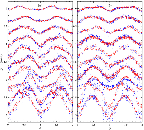
Figure 15. Example LCs for (a) RS CVn and (b) BY Dra stars. The blue filled circles and red plus signs are LCs in the g and r bands, respectively. From top to bottom, the variation amplitudes increase. The mean magnitudes are fixed at 0.3i (i = 0, 1, ..., 9) in the g, r bands for both RS CVn and BY Dra stars.
Download figure:
Standard image High-resolution image
BY Dra stars are also variables featuring chromospheric activity, but they are of K–M type and fainter than RS CVn. Several papers have studied BY Dra and some RS CVn stars based on samples of a few hundred objects (Strassmeier et al. 1993; Eker et al. 2008; Hartman et al. 2011). However, criteria to separate the two types of variables are not well established. In our sample, with the help of Gaia parallaxes, BY Dra stars are predominantly distributed in a narrow magnitude range,  mag (Figure 5). The period range of BY Dra stars is narrower than that of RS CVn variables. As for the overall distributions of periods and amplitudes, both types of variables exhibit similar features. A better study of RS CVn and BY Dra variables will be achieved with a combination of LCs and spectra.
7. Conclusions
ZTF DR2 contains about 0.7 billion objects with more than 20 exposures each. As such, ZTF DR2 represents a highly suitable database for the detection and exploration of new variable stars. In this paper, we have adopted the Lomb–Scargle periodogram approach to search for periodic variables. We obtained a sample of 1.4 million candidates with  . Following exclusion of candidates with aliased periods and poor-quality LCs, ∼1.0 million candidates remained for classification. Classification was done using the DBSCAN method based on the distributions of the objects' periods, LC parameters, and luminosities. We classified 781,602 periodic variables into δ Scuti, EW- and EA-type eclipsing binaries, RRab and RRc Lyrae, classical Cepheids, Type II Cepheids, SRs, and Miras. After cross-matching with known variables, 621,702 of the 781,602 objects turned out to be newly detected variables. This high new detection rate highlights both the high quality of the ZTF photometry and the improvement of our classification method.
Checks of the periods and types contained in our catalog show that they are better than or as good as the same parameters contained in previously published catalogs. The sampling completeness is not homogeneous in the northern sky owing to the observation mode adopted, ranging from 76% at high declinations to 50% in low-declination regions (decl. < 0°). The completeness of LPVs is 30% lower than that of the full sample. For each variable type, our catalog represents a significant increase in sample size. The new variables will aid studies of the physics of variable stars as such, of the Milky Way's structure and evolution, and of the cosmological distance scale, particularly based on a combination of LCs and spectra.
Future ZTF DRs will cover both increased time spans and larger numbers of exposures. These aspects will help improve the determination of the LPV periods and increase the completeness of the catalog. LCs associated with double modes or amplitude (period) modulation will be reanalyzed when enhanced sampling becomes available. In addition to the main types of variables discussed here, there are many cataclysmic variables, low-amplitude pulsating stars, binaries with compact objects, and stars with exoplanets in the ZTF database. These variables will be identified to construct a large sample for further study based on future ZTF DRs.
We thank the anonymous referee for comments that helped us improve the paper. This publication is based on observations obtained with the Samuel Oschin 48-inch Telescope at the Palomar Observatory as part of the Zwicky Transient Facility project. ZTF is supported by the National Science Foundation under grant AST-1440341 and a collaboration including Caltech, IPAC, the Weizmann Institute for Science, the Oskar Klein Center at Stockholm University, the University of Maryland, the University of Washington, Deutsches Elektronen-Synchrotron and Humboldt University, Los Alamos National Laboratories, the TANGO Consortium of Taiwan, the University of Wisconsin at Milwaukee, and Lawrence Berkeley National Laboratories. Operations are conducted by COO, IPAC, and UW. We are grateful for research support from the National Natural Science Foundation of China through grants 11903045, U1631102, and 11633005. This work was supported by the National Key Research and Development Program of China through grant 2017YFA0402702. We also thank Dr. Changqing Luo and Dr. Fan Yang for providing computing time.
Footnotes
- 7
- 8
The period determination process produces half periods for the majority of eclipsing binaries because the two eclipses over a full period are too similar to be separated. Only very few eclipsing binaries with significantly modulated LCs yield full periods.
- 9
The full catalog and LCs can be accessed at http://variables.cn:88/ztf or doi:10.5281/zenodo.3886372.