


Abstract
We describe the PDFI_SS software library, which is designed to find the electric field at the Sun's photosphere from a sequence of vector magnetogram and Doppler velocity measurements and estimates of horizontal velocities obtained from local correlation tracking using the recently upgraded Fourier Local Correlation Tracking code. The library, a collection of FORTRAN subroutines, uses the "PDFI" technique described by Kazachenko et al., but modified for use in spherical, Plate Carrée geometry on a staggered grid. The domain over which solutions are found is a subset of the global spherical surface, defined by user-specified limits of colatitude and longitude. Our staggered grid approach, based on that of Yee, is more conservative and self-consistent compared to the centered, Cartesian grid used by Kazachenko et al. The library can be used to compute an end-to-end solution for electric fields from data taken by the HMI instrument aboard NASA's SDO mission. This capability has been incorporated into the HMI pipeline processing system operating at SDO's Joint Science Operations Center. The library is written in a general and modular way so that the calculations can be customized to modify or delete electric field contributions, or used with other data sets. Other applications include "nudging" numerical models of the solar atmosphere to facilitate assimilative simulations. The library includes an ability to compute "global" (whole-Sun) electric field solutions. The library also includes an ability to compute potential magnetic field solutions in spherical coordinates. This distribution includes a number of test programs that allow the user to test the software.
Export citation and abstract BibTeX RIS
1. Introduction
The goal of this article is to describe the mathematical and numerical details of our software (http://cgem.ssl.berkeley.edu/cgi-bin/cgem/PDFI_SS), which we call PDFI_SS, to derive electric fields in the solar photosphere from a time sequence of vector magnetogram and Doppler shift data (an archived version of the software, available as a gzipped tar file, is also available from Zenodo Fisher et al. 2020b). By reading this paper carefully, the reader should have enough information to understand how to use the software, and also to understand the physical, mathematical, and numerical assumptions that the software employs. For detailed usage of the software, this article is meant to be used in combination with the source code documentation included within each subroutine of the library, along with additional material distributed within the doc folder of the distribution. All source code files include a detailed description of the subroutine arguments, along with expected dimensions and units. For this reason, we do not include the details of subroutine arguments within this article, but we do discuss each important subroutine by name and describe its purpose. It is very easy to view the source code for any subroutine in the PDFI_SS library in a web browser by first going to the above software repository URL, clicking on the "Files" link, and then clicking on the "fortran" folder and then clicking on the links to any of the subroutines.
The PDFI_SS software is based on the PDFI technique for deriving electric fields that is described in detail in Kazachenko et al. (2014, hereafter KFW14). The acronym "PDFI" stands for "poloidal–toroidal decomposition (PTD) plus Doppler plus Fourier local correlation tracking (FLCT) plus ideal" contributions to the electric field. The physical significance of these four electric field contributions will be elaborated in Section 2 of this article. The "_SS" suffix in the name "PDFI_SS" stands for "spherical staggered," because the fundamental differences between the techniques described in KFW14 and those described here are that (1) we use spherical Plate Carrée coordinates instead of Cartesian coordinates, to allow for realistic solar geometries for large domains of the Sun, and (2) we have switched to a staggered grid description of the scalar and vector field variables in the domain. While the basic concepts of KFW14 still apply, there are many differences in the details, which are described in this article.
The development of the PDFI_SS software was motivated by the Coronal Global Evolutionary Model (CGEM), a Strategic Capability Project (http://cgem.ssl.berkeley.edu) funded by NASA's Living With a Star (LWS) Program and by the National Science Foundation (NSF; Fisher et al. 2015). The core activity of the CGEM project is to drive large-scale and active-region-scale magnetofrictional (MF) and magnetohydrodynamic (MHD) simulations of the solar corona using time cadences of vector magnetogram data and electric fields inferred at the photosphere. The PDFI_SS software is what CGEM uses to derive the photospheric electric fields from vector magnetogram and Doppler data that are then used by the MF (Cheung & DeRosa 2012) and RADMHD (Abbett 2007; Abbett & Fisher 2012; Abbett & Bercik 2014) models.
The PDFI_SS software is written as a general purpose library, which can be easily linked to other programs. It is designed to be modular, making it easy for users to customize the software for their own purposes, rather than being written for a single narrow purpose. The PDFI_SS library is written in FORTRAN, primarily because of its extensive use of the FORTRAN library FISHPACK, an elliptic equation package that is well suited to solutions of the 2D Poisson equations that make up the core of the PDFI technique (KFW14). Once compiled, it is straightforward to link the PDFI_SS library to other FORTRAN, C/C++, and Python programs. The SDO Joint Science Operations Center (JSOC) magnetic field pipeline software, which is written in C, calls one of the high-level FORTRAN subroutines within PDFI_SS to compute electric fields within each "CGEM patch" (similar to the "space-weather HMI active region patch," or SHARP; Bobra et al. 2014). Thus, in addition to being a software library, many of the data products that can be computed by PDFI_SS are also available to all users of the SDO JSOC.
The primary purpose of the PDFI_SS library is to compute electric fields in the solar photosphere from time sequences of the input magnetic and Doppler data. The domain of the solutions is a subset of the global solar surface, defined by limits on colatitude and longitude, which we will refer to as the base of a "spherical wedge" domain. However, the software also includes a set of subroutines for performing vector calculus operations on subsets of a spherical surface, it has the ability to compute "nudging" electric fields in a numerical simulation for assimilative purposes, and it also includes the ability to compute 3D potential magnetic field solutions for spherical wedge domains. Within the context of the electric field inversions, the user can customize the electric field solutions by choosing to include or neglect the various contributions to the total PDFI electric field described by KFW14.
In Section 2, we discuss other recently published electric field inversion methods. We then review the PDFI equations for determining electric fields in the solar photosphere from assumed input HMI vector magnetogram and Doppler measurements, along with estimates of flows along the photospheric surface determined from optical flow techniques. We mention spherical geometry corrections to expressions in KFW14 where applicable.
In Section 3, we discuss in detail the numerical implementation of the PDFI solutions, including the staggered grid based on the concepts of Yee (1966), the finite-difference representations, the necessary coordinate transformations and interpolations, and all the other details needed to understand and use the PDFI_SS software to compute electric fields in the photosphere.
In Section 4, we describe the data processing upstream of using PDFI_SS that the software expects to have done before the PDFI electric fields are computed, including corrections for solar rotation and the temporal evolution of the transverse magnetic field from HMI data, corrections to the Doppler velocity from the convective blueshift bias, and the calculation of horizontal velocities from optical flow methods (using FLCT). We include a description of upgrades we have made to the FLCT code for computing horizontal flows. We describe the interpolation of the results to a Plate Carrée grid and the addition of "padding," which improves the properties of the electric field solutions. While the discussion in Section 4 is specific to HMI data, this could be used as a guideline for preparing data sets from other instruments.
In Section 5, we describe broader applications of the PDFI_SS software, beyond the calculation of electric fields described in Section 3. These include the use of "nudging" electric fields for data assimilation in numerical models of the solar atmosphere, the use of curl-free solutions of the electric field to match boundary conditions in other models, and the calculation of global (whole-Sun) solutions for the "PTD" electric field solution.
In Section 6, we describe how to use PDFI_SS to compute potential magnetic field solutions in a spherical wedge domain with a given range in radius between the photosphere and a "source surface." This software differs from most treatments of potential fields in spherical coordinates in that it uses a finite-difference approach rather than spherical harmonic expansion. This same software can be used to compute a 3D distribution of the electric field due to a temporally evolving potential magnetic field in a coronal volume lying above the photosphere, based on the time-dependent behavior of the radial component of the magnetic field at the photosphere.
In Section 7, we describe how to use the PDFI_SS library to compute solutions in Cartesian coordinates, by mapping a small Cartesian patch onto the surface of a very large sphere, with the patch straddling the equator.
In Section 8, we first lay out the development history of the PDFI_SS library and then describe in detail how to compile the PDFI_SS library and then how to link the library to other FORTRAN, C/C++, Python, and legacy IDL software.
In Section 9, we describe test program calculations that are included in the software distribution, including tests of the PDFI_SS solutions using HMI data from NOAA Active Region 11158, an analysis of the ANMHD test data discussed in KFW14 and Schuck (2008), test programs for the potential magnetic field software, tests of the global PTD electric field solutions, and tests of usage of the software from C and Python.
Section 10 contains an alphabetically ordered table (Table 3) of the most important subroutines in the PDFI_SS library, along with lists and descriptions of important commonly used calling argument variables in these subroutines. Table 3 includes a brief description of each subroutine task, along with a link to the section of this article that describes the subroutine in more detail. The objective is to provide the user with an easy-to-use index for specific material within the article.
This article is lengthy, because it is intended to describe in detail all the important aspects of the software. Depending on the reader's goals, it may not be necessary to read the entire article.
If one is simply interested in understanding the "big picture" regarding the PDFI_SS software, one can read KFW14, Section 2, and the first four subsections of Section 3.
If one is interested in using PDFI_SS results obtained from the SDO JSOC, namely, electric field data products computed for selected active regions (ARs), we recommend reading KFW14, plus Sections 2–4.
If one is interested in installing and using the PDFI_SS software to compute electric field solutions from magnetic field data, we recommend reading Sections 2–4 and 7–9.
If one is mainly interested in using PDFI_SS for computing "nudging" electric fields for "data-driving" applications, we recommend reading Sections 2–3, 5, and 8.
If one is only interested in using the potential magnetic field software, we recommend reading Sections 2.1, 6, and 8–9.
If one is only interested in installing and testing the PDFI_SS software, one can simply read Sections 8–9.
2. Review of the PDFI Electric Field Inversion Equations
In their presentation of the PDFI method, KFW14 reviewed the current state of electric field inversions in the literature at the time that paper was published. Since the publication of KFW14, a number of other published efforts for electric field inversions have been done. Here, we first briefly summarize these efforts.
Mackay et al. (2011) and Yardley et al. (2018) solve a Poisson equation for what is effectively a poloidal potential using the time rate of change of the normal magnetic field as a source term, from which one can derive horizontal components of the electric field (expressed in this case by the time derivative of a vector potential). Weinzierl et al. (2016a, 2016b) presented solutions for the horizontal components of the electric field that combined a solution for the "inductive" contributions to the horizontal electric field components, determined from the time derivative of the radial magnetic field, with a noninductive contribution that was determined from surface flux transport models. Yeates (2017) derived electric field solutions that combine solutions for the same inductive contribution as those above, but with the noninductive contribution to the electric field determined from a "sparseness" constraint, to minimize unphysical artifacts of the horizontal electric field from the purely inductive solution. Lumme et al. (2017) and Price et al. (2019) used solutions for all three components of the electric field using time derivatives for all three components of  , as described for the "PTD" solutions in KFW14, using a centered grid formalism. For the noninductive contribution to
  , they used the ad hoc treatments suggested in Cheung & DeRosa (2012). The data-driven MHD simulations of Hayashi et al. (2018, 2019) used solutions for the PTD equations derived in KFW14, evidently including some depth-dependent information for the horizontal electric fields. In Lumme et al. (2019), the full PDFI solutions for all three components of the electric field were determined using the methods described in this article to study the dependence of electric field solutions on time cadence. Lumme et al. (2019) also studied the effect of cadence on solutions determined from the DAVE4VM method (Schuck 2008).
Because of the importance of the curl operator evaluated in spherical coordinates within PDFI_SS, we now explicitly write out each component of the curl before heading into the details of PDFI_SS. This can be found in many standard texts in mathematics, such as Morse & Feshbach (1953). Here we use standard spherical polar coordinates, where the unit vectors are  , pointing in the colatitude direction (i.e., from north to south),
  , pointing in the longitudinal or azimuthal direction (i.e., toward the right, when looking at the equator of the Sun from outside its surface), and
  , pointing in the radial direction (i.e., outward from the center of the Sun). The quantities θ and r are colatitude and radius, respectively. The quantities Uθ, Uϕ, and Ur are the colatitudinal, longitudinal, and radial components of
  , respectively:

and
Since the derivation and discussion of the equations that define the PDFI electric field solutions have already been described in detail in KFW14, we simply review below the equations necessary to define each contribution to the PDFI electric field. The main difference here between KFW14 and these equations is the use of spherical coordinates. The fact that we are using spherical coordinates makes little difference to the overall structure of the equations, but where spherical geometry does change things from Cartesian coordinates, we mention it.
2.1. The PTD Contribution to the Electric Field
We start with the PTD for the magnetic field  in spherical coordinates (Chandrasekhar 1961; Backus 1986) in terms of the poloidal potential P and the toroidal potential T:

where  is the unit vector in the radial direction. Here, in a change from the notation used in KFW14, we use P for the poloidal potential, instead of
  , and T for the toroidal potential, instead of
  . This change was made for notational simplicity and also corresponds with the notation used by Lumme et al. (2017). We also note another useful form for Equation (4), namely,

The operator  is the horizontal Laplacian, i.e., the full Laplacian but omitting the radial derivative contribution, and
  represents the horizontal components of the gradient of the radial derivative of P. By uncurling Equation (4), it is clear that the vector potential
  can be written in terms of P and T as

where we have omitted an explicit gauge term.
The PTD, or "inductive" electric field  , is related to the magnetic field
  through Faraday's law:

where c is the speed of light, and where we use the overdot to denote a partial time derivative. Substituting Equation (4) into Faraday's law and uncurling, we find

where  and
and  are the partial time derivatives of P and T. The general description of the electric field will also include the gradient of a scalar potential in addition to the inductive solution in Equation (8), but we omit any explicit gradient contributions to
  here, and we discuss the gradient contributions in subsections further below.
By evaluating the radial component of Equation (7) when substituting Equation (8) for  , we find that
  obeys the 2D Poisson equation

where Br is the radial magnetic field component. Here, the right-hand side of Equation (9) is viewed as a source term that can be evaluated from the magnetogram data. By taking the radial component of the curl of Equation (7), we find that  obeys the Poisson equation

where  are the horizontal components of
  . A third useful Poisson equation can be found by taking the divergence of the horizontal components of Equation (7):
The quantity  is important because it allows one to evaluate the radial derivative of the horizontal electric field components. To see this, one can evaluate the quantity

where  represents the horizontal components of
  from Equation (8):

The θ and ϕ components of the curl in Equation (13) both contain leading factors of 1/r, as can be seen from the first term of Equation (1) and the second term of Equation (2). The radial derivative in Equation (12) therefore is applied directly to  , resulting in

Expanding the radial derivative on the left-hand side of Equation (14), we then arrive at this expression for the radial derivative of  :
:

Here, the quantity r is the radius of the surface upon which the 2D Poisson equations are solved, which for nearly all of our purposes can be taken as the radius of the Sun R⊙. Equation (15) was not given in KFW14 but, as shown here, is easy to derive. Note that the second term on the right-hand side of Equation (15) goes to zero as  , meaning that in the Cartesian limit, this term vanishes. The radial derivative of the horizontal inductive electric field is useful because it allows one to compute the horizontal components of
  ×
×  .
.
The availability of time cadences of vector magnetic field measurements, such as from the HMI instrument on NASA's SDO Mission (Scherrer et al. 2012), enables the evaluation of the time derivatives as the source terms in the above Poisson equations, making such electric field solutions possible. With the data in hand, evaluation of  becomes a matter of solving the above Poisson equations on a region of the Sun's surface and then evaluating Equation (8).
2.2. Doppler Contributions to the Noninductive Electric Field
The Doppler velocity, when combined with the magnetic field measurements, provides additional information about the electric field beyond the inductive contribution  (Ravindra et al. 2008). The relationship between the measured line-of-sight (LOS) velocity vector
  and the true plasma velocity
  is given by

where  is the LOS unit vector pointing toward the observer from the surface of the Sun. Note that
  is a function of position on the solar surface, since the Sun's surface is curved. Near an LOS polarity inversion line (PIL), the
  flow carrying transverse components of the magnetic field perpendicular to
  results in an electric field contribution

where  represents the components of
  transverse to
  .
.
When we are not near an LOS PIL, a nonzero Doppler velocity is less certain to be coming from a flow that transports  , and instead could be a signature of flows parallel to
  , which have no electric field consequences. To account for this uncertainty away from LOS PILs, the electric field in Equation (17) is modulated by an empirical factor wLOS given by the following expression:

where BLOS is the LOS component of  , and σPIL is an empirically adjustable parameter, commonly taken as unity.
To the extent that the Doppler contribution to the electric field contributes magnetic evolution, that contribution should already have been included in the inductive contribution described in Section 2.1. We therefore want to include any additional curl-free contribution to the electric field from the Doppler term. To do this, we will represent the Doppler contribution in Equation (17) by the gradient of a scalar potential, which we will call ψD:

where we note that this form automatically results in zero curl.
The details of how the equation defining ψD is derived are provided in Section 2.3.3 in KFW14. Here, we will simply write down the result, modified slightly to account for working in spherical, rather than Cartesian, coordinates:
where  is the unit vector pointing in the same direction as
  ×
×  , qr is the radial component of
  , and
, and  are the horizontal components of
  . Equation (20) is solved using the "iterative" technique developed by coauthor Brian Welsch, initially described in Section 3.2 of Fisher et al. (2010), with subsequent changes discussed in Section 2.2 of KFW14. In this article, the current version of the iterative technique for PDFI_SS is described in Section 3.9.2. The iterative technique involves repeated solutions of a 2D Poisson equation that tries to best represent the Doppler electric field from the observed data by the gradient of ψD in the
  -direction.
2.3. FLCT Contributions to the Noninductive Electric Field
There are many techniques currently available to estimate velocities in the directions parallel to the solar surface by solving the "optical flow" problem on pairs of images closely adjacent in time to estimate these flows (see, e.g., reviews by Welsch et al. 2007; Schuck 2008; Tremblay et al. 2018). Here we estimate horizontal flow velocities  using the FLCT local correlation tracking code (Fisher & Welsch 2008) applied to images of Br from the vector magnetogram sequence. The choice of FLCT is somewhat arbitrary; any other existing technique could be used as an alternative. We chose FLCT because we are very familiar with the algorithm and the code and have spent years making the code as computationally efficient as possible.
The use of FLCT in spherical geometry introduces some complications, since the FLCT algorithm is based strictly on assumptions of Cartesian geometry. We adopt the solution proposed in the appendix of Welsch et al. (2009), in which the Br images are mapped to a Mercator projection, FLCT is run, and then the velocities are interpolated and rescaled back to spherical geometry. The FLCT code has been updated to perform this operation automatically if the input data are specified as being equally spaced in longitude and latitude, i.e., on a Plate Carrée grid. More details on recent versions of FLCT can be found in Section 4.4 and in the updated source code and documentation for FLCT, available at the software repository http://cgem.ssl.berkeley.edu/cgi-bin/cgem/FLCT/home.
Horizontal velocities  estimated from FLCT, and acting on the radial component of the magnetic field, provide an additional contribution to the electric field:

We have neglected an additional term, contributing to Er, coming from  in Equation (21). In KFW14, we showed that in Cartesian coordinates this term is already accounted for by the inductive contribution to
  . The same argument applies here, except the contribution is to
  , the radial component.
In regions where the radial magnetic field component is small compared to the horizontal magnetic field components, we trust the FLCT velocities less because the radial magnetic field evolution is less likely to be due to advection by horizontal flows. Therefore, we introduce an empirical modulation function (1−wr) that multiplies the right-hand side of Equation (21) and that reduces the amplitude of the electric field when the magnetic field is mostly horizontal. The quantity wr is given by the expression

where Br is the radial magnetic field component and  are the horizontal magnetic field components. The empirical factor σPIL is the same empirical factor (typically unity) used in the above discussion of the electric field from the Doppler velocity.
To avoid including inductive electric fields that are already accounted for by  , we remove any inductive contributions by writing the FLCT-derived electric field in terms of the gradient of a scalar potential ψF:

To derive an equation for ψF, we can take the horizontal divergence of  and set it equal to the divergence of
  , where
  is taken from Equation (21):

Once this Poisson equation is solved for ψF,  can be evaluated from Equation (23).
2.4. "Ideal" Corrections to the Electric Field Solutions
Most of the time, we expect that electric fields in the solar photosphere will be largely determined by the electric field in ideal MHD, namely,  , where
  is the local plasma velocity. A consequence of this is that we expect
  . However, we found that if the PTD (inductive) contribution, Doppler contribution, and FLCT contribution are added together, the resulting electric field can have a significant component parallel to the direction of
  . We therefore want to find a way to add a scalar potential electric field

such that

where  is the sum of the PTD (inductive), Doppler, and FLCT electric field contributions. When
  is added to the electric field, the result should have
  , where
  is now the complete PDFI electric field solution. In Section 2.2 of KFW14, the equation that ψI and its depth derivative obey is given in Equation (19) of that article. The form of the equation is changed only slightly in spherical coordinates and is

Here,  is the unit vector pointing in the direction of
  , and br and
  are the radial and horizontal components of
  , respectively. As described in Section 2.2 of KFW14, Equation (27) is solved using the "iterative" technique, also mentioned earlier in Section 2.2 of this article, with further details given in Section 3.9.2. Once ψI and ∂ψI/∂r have been found, the full PDFI solution is given by
It is important to note that this same procedure to "perpendicularize"  with respect to
  can be performed with any combination of the other electric field contributions. For example, in cases where there are no Doppler or FLCT velocity flows available, one can substitute
  for
for  in Equations (27)–(28) to generate an electric field solution that should still minimize
  . This is described in detail in Section 2.3.4 of KFW14 (see also Table 1 of KFW14).
Once the PDFI electric fields have been computed, we can use them to estimate the Poynting flux of energy in the radial direction:

We can also compute the helicity injection rate contribution function, hr:

where  , and the poloidal potential P is found from Equation (9) but without the time derivative in the source term. The relative helicity injection rate was derived by Berger & Field (1984) in terms of a surface integral of Equation (30). Schuck & Antiochos (2019) argue that integrating over a finite area, as we do here, and neglecting the other surfaces of our spherical wedge volume domain may result in a loss of gauge invariance. For the time being, we ignore this possible complication and simply use Equation (30) as an integrand to estimate the helicity injection rate. Berger & Hornig (2018) have pointed out that using the PTD formalism for describing the magnetic field, which we employ for computing the inductive contribution to the electric field, has some useful properties. The magnetic helicity in a volume can be understood in terms of the linkage between the contribution to the magnetic field generated by the poloidal potential and that generated from the toroidal potential. That analysis also leads to the same surface integral of the quantity in Equation (30) for the relative helicity injection rate, assuming that the volume integral of
  is zero if the coronal plasma is described by ideal MHD, and that the contributions from the other surfaces surrounding the volume can be neglected.
KFW14 studied the accuracy of the PDFI electric field solutions, as well as the Poynting flux and Helicity injection rates, for the case of an MHD simulation of magnetic flux emergence in a convecting medium, originally described by Welsch et al. (2007). They found that including the PTD, Doppler, FLCT, and ideal electric field contributions (in other words, the full PDFI electric field) resulted in the most accurate reconstruction of the electric field from the MHD simulation. The comparison is described in detail in Section 4 of KFW14. For details of tests of the PDFI solution from these simulation data using PDFI_SS, see Section 9.2.
3. Numerical Solution of PDFI Equations in PDFI_SS
The fundamental mathematical operations of the PDFI software are the solution of the Poisson equation in finite domains in a 2D geometry, where the source terms depend on observed data, and then the evaluation of electric field contributions that are either the curl of the solution multiplying  or the gradient of the solution in two dimensions. Since solving the Poisson equation plays such a central role in PDFI_SS, it is worth noting and describing the software we have chosen.
In KFW14, and in this article, we have chosen version 4.1 of the FISHPACK FORTRAN library to perform the needed solutions of the Poisson equation. FISHPACK is a package that was developed at NCAR many years ago for the general solution of elliptic equations in two and three dimensions. We find that the code is extremely efficient and accurate and includes many different possible boundary conditions that are ideally suited for use on the PDFI problem. In KFW14, we used subroutines from the package that were designed for Cartesian geometry; for PDFI_SS, we use subroutines from FISHPACK designed for the solution of Helmholtz or Poisson equations in subdomains placed on the surface of a sphere. The partial differential equations are approximated by second-order-accurate finite-difference equations; the solutions FISHPACK finds are of the corresponding finite-difference equations.
Version 4.1 of FISHPACK can be downloaded from NCAR at https://www2.cisl.ucar.edu/resources/legacy/fishpack/documentation. A copy of the tarball for version 4.1 can also be downloaded from http://cgem.ssl.berkeley.edu/~fisher/public/software/Fishpack4.1/. The source code has well-documented descriptions of all the calling arguments used by the subroutines contained in the software. A very useful document describing an older version of the software is the NCAR Tech Note IA-109 (Swarztrauber & Sweet 1975), which contains valuable technical information about FISHPACK that is not described elsewhere. The numerical technique of "cyclic reduction" for solving the Poisson equations in general, as well as on the surface of a sphere, is described by Sweet (1974), Swarztrauber (1974), and Schumann & Sweet (1976).
A notable feature of the FISHPACK software for Cartesian and spherical domains is that there exist different subroutines for solving Poisson equations that use either a centered or a staggered grid assumption, that is, whether the equations are solved at the vertices of cells or centers of cells, respectively. This ability is very useful for PDFI_SS, as will be described in further detail below in the remainder of Section 3.
3.1. FISHPACK Domain Assumptions and Nomenclature Used in PDFI_SS
The Helmholtz/Poisson equation subroutines for spherical coordinates in FISHPACK are named HSTSSP (the staggered grid case) and HWSSSP (the centered grid case). Important input arguments to these subroutines include the source term for the Poisson equation (a 2D array) and boundary conditions applied to the four edges of the problem domain (four 1D arrays). Note that the FISHPACK software assumes that the Poisson equation is multiplied by r2 (where r is the radius), meaning that the source terms of all Poisson equations in PDFI_SS must also be multiplied by r2 before calls to HSTSSP and HWSSSP. The boundary conditions most useful to PDFI_SS include the specification of derivatives of the solution in the directions normal to the domain boundary edges (Neumann boundary conditions). The problem domain is described further below. Both of these subroutines make certain assumptions about the geometry of the domain, the array dimensions, and how the arrays are ordered. To avoid confusion, we adopt exactly the same nomenclature that is used in FISHPACK throughout our software to describe the domain, its boundaries, and the grid spacing.
Spherical coordinates in FISHPACK assume spherical polar coordinates, with the first independent variable θ being colatitude and the second independent variable ϕ being azimuthal angle (longitude). See Section 3.2 and the figures in Section 3.4 for a comparison between spherical polar coordinates and the longitude–latitude coordinate system typically used to display magnetic field data.
Both colatitude and longitude are measured in radians. Colatitude θ ranges from 0 (North Pole) to π (South Pole). Longitude ϕ ranges from 0 to 2π, with negative values of longitude not allowed within these two subroutines. The finite-difference approximations to the Poisson equations are solved in a domain where the edges of the domain are defined by lines of constant colatitude and constant longitude. The northern edge of the domain is defined by θ = a and the southern edge of the domain by θ = b, where 0 < a < b < π. The leftmost edge of the domain is defined by ϕ = c, and the rightmost edge of the domain is defined by ϕ = d, where 0 < c < d < 2π.
In the colatitude direction, there are a finite number of cells, denoted m. In the longitude direction, there are a finite number of cells, denoted n. The angular extent of a cell in each direction is assumed constant, and these angular thicknesses are given by the following expressions:

and

If we are using the staggered grid case, the number of variables in each direction is the number of cell centers; so in this case, solution arrays (without ghost cells) will have dimensions of (m, n). If we are assuming the centered grid case, the number of variables in each direction is the number of cell edges, which is one greater than the number of cell centers. In that case, the solution arrays (without ghost zones) will have dimensions of (m + 1, n + 1).
The quantities a, b, c, d, m, n, Δθ, and Δϕ will retain the meanings defined here throughout the rest of this article.
3.2. Transposing between Solar and Spherical Polar Array Orientation
Given the implicit assumption in FISHPACK of spherical polar coordinates (colatitude and longitude) and the default assumption used nearly universally in solar physics of longitude–latitude array orientation, we are led immediately to the need for frequently transforming back and forth between longitude–latitude and colatitude–longitude array orientations. Thus, an important part of the PDFI_SS software consists of the ability to perform these transpose operations easily and routinely. Detailed discussion of the subroutines that perform these operations is described in Section 3.6 of this article; here we simply present a high-level view of where these transpose operations must be done.
First, if we are using vector magnetogram and Doppler data from HMI on SDO, these data are automatically provided in longitude–latitude orientation. Therefore, a first step is to transpose all the input data (vector magnetograms, velocity maps, LOS unit vectors) to colatitude–longitude orientation. Then, the PDFI solutions are obtained using FISHPACK software in colatitude–longitude order. Essentially all mathematical operations on the data and electric field solutions are done in colatitude–longitude orientation. Finally, because users expect the solutions to be in the same orientation as the HMI data, we must transpose computed results in the other direction to provide the electric field solutions and other related quantities in longitude–latitude order.
For further details, see Section 3.6.
3.3. Advantages of Using a Staggered Grid over a Centered Grid for PDFI
In KFW14, we used a centered grid definition for finite-difference expressions for first derivatives (Equations (14)–(15) in KFW14) in the horizontal directions in our definitions for the curl and gradient. On the other hand, we also used a standard five-point expression for the Laplacian (Equation (16) in KFW14, also used by the Cartesian FISHPACK Poisson solver), which uses centered grid expressions for second derivatives. However, Equation (16) from KFW14 implicitly uses first-derivative finite-difference expressions that are centered half a grid point away from the central point. This means that there is an inconsistency between Equations (16) and (14)–(15) in KFW14. This inconsistency shows up when one uses the centered finite-difference expressions to evaluate  and compares it to
  using Equation (16) in KFW14. In the continuum limit, the two expressions should be identical, but the finite-difference approximations are not equal; the double curl expression using centered finite differences for first derivatives yields an expression like Equation (16) of KFW14, but with the grid points separated by 2Δx and 2Δy. If the grid resolves the solution well, the two different expressions will not differ greatly. This, in fact, is the case with the ANMHD simulation data analyzed in KFW14. But if the solution has structure on the same scale as the grid separation, the double curl expression and the horizontal Laplacian expression can differ significantly, rendering solutions to the PDFI equations quite inaccurate. This problem exists for both the Cartesian and spherical versions of the PDFI equations.
To illustrate the problem quantitatively, we have constructed a solution in spherical coordinates to the Poisson Equation (9) using a centered grid formulation of the finite differences, then evaluated  from the horizontal components of Equation (8), and then evaluated
  , which should be equal to the input source term,
  . In this case, the input source term is taken to be a field of random numbers ranging from −0.5 to 0.5, which has significant structure on the scale of the grid. Figure 1 shows an image of the original field of the assumed
  . Figure 2 shows a point-by-point scatterplot of the "recovered" versus original values of
  , showing about half the correct slope, and random errors of roughly 50%. The recovered values of
  were computed as described above using the centered grid finite-difference expressions. Examination of Figure 2 shows that the centered grid finite-difference expressions do a poor job of describing the correct solution for this test case. The behavior of this test case is similar to what we might expect if the source term has significant levels of pixel-to-pixel noise, which is the case with real magnetogram data in weak-field regions.
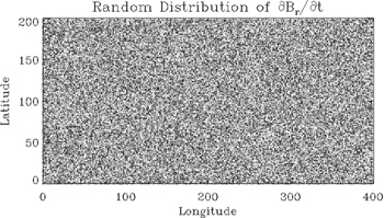
Figure 1. Input distribution of the test  configuration, displayed in longitude–latitude order. This case has m = 200, n = 400, a = π/2 − 0.1, b = π/2 + 0.1, c = 0, and d = 0.4. The input distribution is a field of random numbers distributed between −0.5 and 0.5.
Download figure:
Standard image High-resolution image
Figure 2. Recovered field of  plotted vs. the input field of
  for the centered grid case shown in Figure 1.
Download figure:
Standard image High-resolution imageBy changing the definition of how finite-difference approximations to spatial derivatives are defined, and where different variables are located within the grid, we can improve this behavior dramatically. In the centered grid case, all variables are colocated at the same grid points. By defining the radial magnetic field and its time derivative to lie at the centers of cells, with the electric field components lying on the edges (or "rails") surrounding the cells, the finite-difference approximations to the derivatives can be made to obey Faraday's law to floating-point roundoff error. Figure 3 shows the analogous scatterplot shown in Figure 2, but using the staggered grid definition described above. The relationship is a straight line. Figure 4 shows the difference between the recovered and original values of  . Note that the amplitude of the error is multiplied by 1 × 10¹², so that the error term is visible in the scatterplot. These two plots clearly show that solutions for the electric fields in a staggered grid formulation can do a far better job of representing the observed data than can the centered grid formulation.

Figure 3. Recovered field of  plotted vs. the input field of
  for the staggered grid test case.
Download figure:
Standard image High-resolution image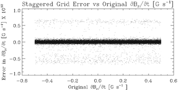
Figure 4. Difference between recovered  and input
  as a function of the input
  for the staggered grid case.
Download figure:
Standard image High-resolution imageThese figures motivate the development of our more detailed staggered grid formalism, which is described in Section 3.4.
3.4. The Staggered Grid Formulation for PDFI_SS
In three dimensions, Yee (1966) worked out a second-order-accurate finite-difference formulation for Maxwell's equations, pointing out that if one places different variables into different locations within the grid, the governing continuum equations (the curls in Maxwell's equations) become conservative when written down in a finite-difference form. In recent years, "mimetic methods" have been developed, which are higher-order analogs to the Yee grid, in that different variables are defined at different locations within a voxel (such as at interiors, faces, or edges), and with some internal structure in these voxel subdomains allowed. The locations of the variables depend on which integral conservation law is being applied (see, e.g., Candelaresi et al. 2014 and references therein). For our work, the second-order-accurate Yee grid is sufficient. The Yee grid is the basis for the numerical implementation of the MF code described by Cheung & DeRosa (2012).
In PDFI_SS, we have a slightly different situation, where most of the calculations are defined on a subdomain of a spherical surface, so that the domain is 2D, rather than 3D. Nevertheless, the exercise shown in Section 3.3 shows that we want to use the advantages of a staggered grid description of the finite-difference equations, which is inspired by the Yee grid. This is complicated by the fact that in addition to needing curl contributions to the electric field (see Section 2.1), we also need to represent gradient contributions to the electric field (Sections 2.2–2.4). This must be done in such a way that both contributions are colocated along the rails that surround a cell center. We found a way to satisfy these constraints with a specific staggered grid arrangement of the physical and mathematical variables within our 2D domain, summarized below.
First, we define six different grid locations for variables in PDFI_SS, illustrated schematically in Figures 5 and 6. For the moment, we use colatitude–longitude array index order in this discussion. We define the CE grid locations as being the centers of the 2D cells; the CE grid variables are dimensioned (m, n). Next, we define the interior corner grid locations, the "CO" grid, as residing at all the corners, or vertices of the cells, but specifically not including the vertices that lie along the domain edges. Variables lying on the CO grid will have dimension (m − 1, n − 1). Next, we define the "COE" grid, which is also located along corners of cells, but in this case the corners that lie along the domain edges are included. Variables lying on the COE grid will have dimension (m + 1, n + 1). Variables that lie along cell edges that have constant values of ϕ (or longitude) but are at midpoints in θ (or colatitude) lie on the "PE" (phi-edge) locations of the domain. Variables at PE locations have dimension (m, n + 1). Variables that lie along edges with constant θ (or colatitude) but are at midpoints in ϕ lie on the "TE" (theta-edge) grid locations. Variables at TE locations have dimension (m + 1, n). Finally, if we are describing these grid locations, but using longitude–latitude index order, the dimensions of the variables are just the reverse of the dimensions given above.
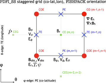
Figure 5. Schematic diagram of our staggered grid, based on the Yee grid concept, oriented in spherical polar (colatitude–longitude) orientation. This figure shows the grid near the leftmost, northern domain corner, oriented in the θ–ϕ (colatitude–longitude) directions. The x-axis increases in the colatitude direction, and the y-axis increases in the longitude direction. The CE, CEG, CO, COE, TE, and PE grid locations are shown, along with where some of the physical variables are located on these grids.
Download figure:
Standard image High-resolution image
Figure 6. Schematic diagram of our staggered grid, based on the Yee grid concept, oriented in longitude–latitude (i.e., "solar") orientation. This figure shows the grid near the leftmost and southern domain corner. The x-axis increases in the longitude direction, and the y-axis increases in the latitude direction. The CE, CEG, CO, COE, TE, and PE grid locations are shown, along with where some of the physical variables are located on these grids.
Download figure:
Standard image High-resolution imageHere are some examples of where different physical and mathematical variables are located using these grid definitions: Br and  are located on the CE grid, Bθ and Eϕ are located on the TE grid, Bϕ and Eθ are located along the PE grid, Er and
  are located along the COE grid, and
  is located along the CO grid. The scalar potentials defined in the PDFI equations (Sections 2.2–2.4) are located on the COE grid. The poloidal potential
  is in principle located along the CE grid (with dimensions (m, n)), but we find it convenient to add ghost zones to
  to implement Neumann (derivative-specified) boundary conditions. When that is done, we refer to this grid as a "CEG" grid (CE plus ghost zones).
  is on the CEG grid and has dimensions of (m + 2, n + 2).
The placement of variables into the staggered grid locations described above is very similar to the placement used in the "constrained transport" MHD model of Stone & Norman (1992a, 1992b) and the filament construction model of van Ballegooijen (2004). Table 1 contains a list of variables in PDFI_SS and where they reside in terms of these grid locations.
Table 1. PDFI_SS Variable Locations and Dimensions
| Quantity | Grid | Dimension (tp) | Dimension (ll) |
|---|---|---|---|
| Input Data | COE | (m + 1, n + 1) | (n + 1, m + 1) |

|
CE | (m, n) | (n, m) |

|
TE | (m + 1, n) | (n, m + 1) |

|
PE | (m, n + 1) | (n + 1, m) |
| Vθ | TE | (m + 1, n) | (n, m + 1) |
| Vϕ | PE | (m, n + 1) | (n + 1, m) |
| VLOS | COE | (m + 1, n + 1) | (n + 1, m + 1) |

|
COE | (m + 1, n + 1) | (n + 1, m + 1) |
| Er | COE | (m + 1, n + 1) | (n + 1, m + 1) |
| Eθ | PE | (m, n + 1) | (n + 1, m) |
| Eϕ | TE | (m + 1, n) | (n, m + 1) |

|
CEG | (m + 2, n + 2) | (n + 2, m + 2) |

|
CEG | (m + 2, n + 2) | (n + 2, m + 2) |

|
COE | (m + 1, n + 1) | (n + 1, m + 1) |
| ψ | COE | (m + 1, n + 1) | (n + 1, m + 1) |

|
CE | (m, n) | (n, m) |

|
CO | (m − 1, n − 1) | (n − 1, m − 1) |

|
CE | (m, n) | (n, m) |

|
CO | (m − 1, n − 1) | (n − 1, m − 1) |
| Sr | CE | (m, n) | (n, m) |
| Hm | CE | (m, n) | (n, m) |
| MCOE | COE | (m + 1, n + 1) | (n + 1, m + 1) |
| MCO | CO | (m − 1, n − 1) | (n − 1, m − 1) |
| MTE | TE | (m + 1, n) | (n, m + 1) |
| MPE | PE | (m, n + 1) | (n + 1, m) |
| MCE | CE | (m, n) | (n, m) |
Download table as: ASCIITypeset image
3.5. Units Assumed by PDFI_SS Software Library
It is assumed by the PDFI_SS library that all magnetic field components on input to the library subroutines are in units of Gauss (G). Units of length are determined by the radius of the Sun, which is assumed to be given in kilometers (km). For solar calculations in spherical coordinates, we expect R⊙ to be 6.96 × 10⁵ km, although in the software the radius of the Sun is an input parameter that can be set by the user. Units of time are assumed to be in seconds (s). Velocities are assumed to be expressed in units of km s−1. For the "working" units of the electric field, the electric field is evaluated as  , i.e., the speed of light times the electric field vector, with each component having units of G km s−1. The subroutines that compute the Poynting flux and the Helicity injection rate contribution function are exceptions to this rule and assume that electric field components on input are expressed in units of volts per cm (V cm−1). To convert from G km s−1 to V cm−1, one can simply divide by 1000. To convert units in the opposite direction, one would multiply by 1000.
3.6. Time Derivatives, Transpose, Interpolation, and Masking Operations in PDFI_SS
We mentioned in Section 3.2 that transpose operations from longitude–latitude array orientation to spherical polar coordinates (and the reverse) would need to be done frequently. Now that we have introduced our staggered grid definitions, we will describe in detail how these operations are done, as well as how the interpolation from the input data grid to the staggered grid locations is done. We will discuss how time derivatives are estimated, as well as the calculation of the strong magnetic field masks, designed to decrease the effects of noise from the magnetic field measurements in weak-field regions on the electric field solutions.
The source terms for the PTD contribution to the electric field (Section 2.1) consist of time derivatives of magnetic field components. To estimate these time derivatives from the data, we simply difference the magnetic field values at their staggered grid locations between two adjacent measurement times and divide by the cadence time period, Δt. Thus, if we have magnetic field measurements at times t0 and t1 = t0 + Δt, then our electric field solution will be evaluated at time  and will be assumed to apply over the entire time interval between t0 and t1. Furthermore, we assume that the magnetic field values needed to evaluate the other electric field contributions (Sections 2.2–2.4) will be the magnetic field values at
  , which will be an average of the input values at the two times. Similarly, the other input variables that affect the calculation of
  will also be an average of the variables at the two adjacent times. If our electric field solutions are conservative and accurately obey Faraday's law, then the computed electric field solutions should correctly evolve
  from t0 to t0 + Δt = t1 with minimal error.
Thus, for a single time step, the needed input data to evaluate the PDFI solutions are arrays of Br, Bθ, Bϕ, VLOS, Vθ, Vϕ, ℓr, ℓθ, and ℓϕ at two adjacent measurement times, for a total of 18 input arrays. Because of the FISHPACK spherical coordinate solution constraints, the data will have to be evaluated using equally spaced colatitude and longitude grid separations, meaning constant spacing in Δθ and Δϕ, referred to as a "Plate Carrée" grid. In the case of HMI data from SDO, this is one of the standard mapping outputs for the magnetic field and Doppler measurements. For CGEM calculations of the electric field supported by the SDO JSOC, the values of Δθ and Δϕ are set to 0 03 in heliographic coordinates (converted to radians), coinciding closely with an HMI pixel size near disk center. The PDFI_SS software can accommodate values of Δθ and Δϕ that differ, but the FLCT software used upstream of PDFI_SS needs to have these values equal to one another. The JSOC software produces Plate Carrée data with Δθ = Δϕ.
We now briefly digress to describe the relationship between the mathematical coordinate system used by PDFI_SS, with angular domain limits a, b, c, and d, and the standard WCS keywords CRPIX1, CRPIX2, CRVAL1, CRVAL2, CDELT1, and CDELT2 that describe the position of the HMI data on the solar disk (Thompson 2006). We want the ability to concisely relate these two descriptions to each other. The quantities CRPIX1 and CRPIX2 denote longitude and latitude reference pixel locations (the center of the field of view measured from the lower left pixel at (1,1)), CRVAL1 and CRVAL2 denote the longitude and latitude (in degrees) of the reference pixel, and CDELT1 and CDELT2 denote the number of degrees in longitude and latitude between adjacent pixels. From the above description, we expect that CDELT1 and CDELT2 will be equal to 003 pixel–1. We have written three subroutines, abcd2wcs_ss, wcs2mn_ss, and wcs2abcd_ss, the first of which converts a, b, c, d, m, and n to the WCS keywords CRPIX1, CRPIX2, CRVAL1, CRVAL2, CDELT1, and CDELT2; and in the reverse direction, wcs2mn_ss, which finds m and n from CRPIX1 and CRPIX2 for the COE grid, and wcs2abcd_ss, which converts the keywords CRVAL1, CRVAL2, CDELT1, and CDELT2 to a, b, c, and d. The subroutine abcd2wcs_ss computes the reference pixel locations CRPIX1 and CRPIX2 for all six grid cases, namely, the COE, CO, CE, CEG, TE, and PE grids. These results for the reference pixel locations are returned as six-element arrays, in the order given above.
Returning the discussion to how the input data arrays are processed, the data arrays, in longitude–latitude order, are assumed to be dimensioned (n + 1, m + 1), with all nine input arrays for each of the two times being colocated in space. The parameter a is the colatitude of the northernmost points in these arrays, and the parameter b is the colatitude of the southernmost points in the arrays. The parameters c and d are the leftmost and rightmost longitudes of the input arrays, respectively.
The first task is to transpose all 18 arrays from longitude–latitude to colatitude–longitude (spherical polar coordinates, or θ − ϕ order.) Basically, the transpose operation looks like

where j ∈ [0, n] and i ∈ [0, m], and where Atp is the array in θ − ϕ index order and Aℓℓ is the array in longitude–latitude order. Here "tp" in the subscript is meant as a shorthand for "theta-phi," and "ℓℓ" is meant as a shorthand for "longitude–latitude." An exception is for those arrays that represent the latitude components of a vector (like Blat), in which case when transforming to Bθ the overall sign must also be changed since the unit vectors in latitude and colatitude directions point in opposite directions.
PDFI_SS has several subroutines to perform these transpose operations (and their reverse operations) on the COE grid, namely, brll2tp_ss bhll2tp_ss brtp2ll_ss bhtp2ll_ss.
Here the subroutines starting with "br" perform the transpose operation on scalar fields, while the subroutines starting with "bh" perform the transpose operations on pairs of arrays of the horizontal components of vectors. Subroutines containing the substring "ll2tp" perform the transpose operation going from longitude–latitude order to theta-phi (colatitude–longitude) order, while those with the substring "tp2ll" go in the reverse direction. When going from the input data to colatitude–longitude order, we use the subroutines containing ll2tp within their name. When examining the source code, the expressions will differ slightly from that in Equation (33) to conform with the default FORTRAN index range (where index numbering starts from 1).
Once the input data arrays on the COE grid have been transposed to colatitude–longitude order, we then interpolate the data to their staggered grid locations. Br is interpolated to the CE grid, Bθ and Vθ to the TE grid, and Bϕ and Vϕ to the PE grid. In addition, to evaluate the FLCT electric field contribution, we also need to have Br and  interpolated to both the TE and PE grids. Here, we use a simple linear interpolation, as given in these examples for the magnetic field components:

and

The interpolations from the input data arrays on the COE grid to the staggered grid locations can be accomplished with the subroutines interp_data_ss interp_var_ss.
The linear interpolation is a conservative choice and results in a slight increase in signal-to-noise ratio if there is a high level of pixel-to-pixel noise variation. This interpolation slightly decouples the PDFI_SS electric field from the original input data on the COE grid: the near-perfect reproduction of  applies for the interpolations to cell center, but not necessarily for the original input Br at COE locations.
The Doppler velocity and the LOS unit vector input data arrays are kept at the COE grid locations, so no interpolation of these data arrays is necessary.
In addition to interpolating the input data to the staggered grid locations, we must also construct masks, based on the input data, that reflect regions of the domain where we expect that noise in the magnetic field measurements will make the electric field calculation unreliable. In PDFI_SS the criterion for masks on the magnetic field variables is determined by a threshold on the absolute magnetic field strength, including radial and horizontal components. The mask value is set to unity if the absolute value of the magnetic field in the input data is greater than a chosen threshold for both of the time steps; otherwise, the mask value is set to zero. This calculation is done on the COE grid, after the transpose from longitude–latitude to theta-phi array order. The subroutine that does this is
find_mask_ss.
Subroutine find_mask_ss was originally written assuming that we were using data from three separate time steps, rather than the two time steps we now use. We now simply repeat the array inputs for one of the two time steps, which then results in the correct behavior. For HMI vector magnetogram data, we currently use a threshold value bmin of 250 G. The threshold value is a calling argument to the subroutine and thus can be controlled by the user.
We need to have mask arrays for all the staggered grid locations, not just the COE grid. To get mask arrays for the CE, TE, and PE locations and array sizes, we use a two-step process. First, we use the subroutine interp_var_ss to interpolate the COE mask array to the other staggered grid locations. Those interpolated points where input mask values transition between 0 and 1 will have mask values that are between 0 and 1. The subroutine fix_mask_ss can then be used to set intermediate mask values to either 0 or 1, depending on the value of a "flag" argument to the subroutine, which can be either 0 or 1. Setting flag to 0 is the more conservative choice, while setting flag to 1 is more trusting of the data near the mask edge values.
Once the strong magnetic field mask arrays have been computed, they can be used to multiply the corresponding magnetic field or magnetic field time derivative arrays on input to the subroutines that calculate electric field contributions. This can significantly reduce the impact of magnetogram noise on the electric field solutions in weak magnetic field regions of the domain.
We denote the mask arrays coinciding with different grid locations with the following notation: MCOE is the mask on the COE grid, MCO denotes the mask on the CO grid, and MTE, MPE, and MCE denote the masks for the TE, PE, and CE grid locations, respectively. The mask arrays are also shown in Table 1.
Once electric field solutions have been computed in spherical polar coordinates, we need the ability to transpose these arrays, as well as the staggered grid magnetic field arrays, back to longitude–latitude order. Because the array sizes are all slightly different depending on which grid is used for a given variable, we have written a series of subroutines designed to perform the transpose operations on our staggered grid, depending on variable type and grid location. There are subroutines to go from theta-phi (colatitude–longitude) order to longitude–latitude order, as well as those that go in the reverse direction. The subroutines that perform the transpose operations on staggered grid locations all have the substring "yee" in their name. As before, subroutine names that include a substring of "tp2ll" transpose the arrays from theta-phi to longitude–latitude array order, while those with "ll2tp" go in the reverse direction. The subroutines are bhyeell2tp_ss bryeell2tp_ss bhyeetp2ll_ss bryeetp2ll_ss ehyeell2tp_ss eryeell2tp_ss ehyeetp2ll_ss eryeetp2ll_ss.
3.7. Vector Calculus Operations Using the PDFI_SS Staggered Grid
Now that we have established how to generate input data on the staggered grid locations in spherical polar coordinates, we are ready to discuss how to perform vector calculus operations on those data. These operations are used inside the software that evaluates various electric field contributions, and they can also be used to perform other calculations using the electric field solutions.
The following expressions are the continuum vector calculus operations in spherical polar coordinates that are important in evaluating the PDFI equations of Section 2:
where Ψ is a scalar function defined in the θ, ϕ domain,


where  is an arbitrary vector field and
  represents the divergence in the horizontal directions, and finally
Here Uθ and Uϕ are the θ and ϕ components of  .
.
We now convert these differential expressions to finite-difference expressions, evaluated at various different grid locations in our staggered grid system. Many of these expressions must be evaluated separately depending on where the variables are located, or where we want the expression to be centered. For example, we will need to evaluate Equation (41) at both cell centers (the CE grid) and interior corners (the CO grid), and the exact expressions will differ depending on where the equations are centered.
The subroutines that evaluate the finite-difference expressions corresponding to the above equations are curl_psi_rhat_co_ss curl_psi_rhat_ce_ss gradh_co_ss gradh_ce_ss divh_co_ss divh_ce_ss curlh_co_ss curlh_ce_ss delh2_ce_ss delh2_co_ss.
These subroutines are discussed in more detail below.
In the following equations, we will use this notation to distinguish quantities lying along an edge, versus halfway between edges: an index denoted i or j denotes a location at a θ or ϕ edge, respectively, while an index denoted i +  or j +
  denotes a location halfway between edges. For example, a quantity defined on the CO grid will have indices i, j, while a quantity defined on the CE grid will have indices
  . Similarly, a quantity defined on the TE grid will have the mixed index notation
  , and one along the PE grid would have an index notation of
  .
.
We will start by evaluating Equation (38) assuming that the scalar field Ψ lies on the COE grid. An example of this case is evaluating the curl of the toroidal potential T times  to find its contribution to the horizontal components of the magnetic field (see Equation (4)). Setting
  , we find

for i ∈ [0, m] and for ![$j+\tfrac{1}{2}\in \left[\tfrac{1}{2},n-\tfrac{1}{2}\right]$](https://content.cld.iop.org/journals/0067-0049/248/1/2/revision1/apjsab8303ieqn135.gif) and
and
for ![$i+\tfrac{1}{2}\in \left[\tfrac{1}{2},m-\tfrac{1}{2}\right]$](https://content.cld.iop.org/journals/0067-0049/248/1/2/revision1/apjsab8303ieqn136.gif) and for j ∈ [0, n]. Here, Uθ is dimensioned (m + 1, n) and is defined on the TE grid, while Uϕ is dimensioned (m, n + 1) and lies on the PE grid. To evaluate Equations (42) and (43), one can use subroutine curl_psi_rhat_co_ss from the PDFI_SS library.
and for j ∈ [0, n]. Here, Uθ is dimensioned (m + 1, n) and is defined on the TE grid, while Uϕ is dimensioned (m, n + 1) and lies on the PE grid. To evaluate Equations (42) and (43), one can use subroutine curl_psi_rhat_co_ss from the PDFI_SS library.
If Ψ is defined on the CEG grid, this has an array size of (m + 2, n + 2), and we then have
for ![$i+\displaystyle \frac{1}{2}\in \left[\displaystyle \frac{1}{2},m-\displaystyle \frac{1}{2}\right]$](https://content.cld.iop.org/journals/0067-0049/248/1/2/revision1/apjsab8303ieqn137.gif) and for j ∈ [0, n] and
and for j ∈ [0, n] and
for i ∈ [0, m] and for ![$j+\tfrac{1}{2}\in \left[\tfrac{1}{2},n-\tfrac{1}{2}\right]$](https://content.cld.iop.org/journals/0067-0049/248/1/2/revision1/apjsab8303ieqn138.gif) .
.
Here, Uθ is dimensioned (m, n + 1) and lies on the PE grid, while Uϕ is dimensioned (m + 1, n) and lies on the TE grid. In these expressions, array values of ΨCEG at  and
and  refer to the ghost zone values (with similar expressions for i +
  ). To evaluate Equations (44) and (45), one can use subroutine curl_psi_rhat_ce_ss.
Note that these expressions require the evaluation of  at both edge locations and at cell centers in θ. The need for these geometric factors is ubiquitous in PDFI_SS, so we have written a subroutine sinthta_ss
to precompute these array values before calling many of the vector calculus subroutines.
Turning now to the discretization of Equation (39), namely, evaluating  , the finite-difference expressions for Ψ lying on the COE grid are

where ![$i+\tfrac{1}{2}\in \left[\tfrac{1}{2},m-\tfrac{1}{2}\right]$](https://content.cld.iop.org/journals/0067-0049/248/1/2/revision1/apjsab8303ieqn144.gif) and j ∈ [0, n], and
and j ∈ [0, n], and

where i ∈ [0, m] and ![$j+\tfrac{1}{2}\in \left[\tfrac{1}{2},n-\tfrac{1}{2}\right]$](https://content.cld.iop.org/journals/0067-0049/248/1/2/revision1/apjsab8303ieqn145.gif) . In this case Uθ is dimensioned (m, n + 1) and lies on the PE grid, while Uϕ is dimensioned (m + 1, n) and lies on the TE grid. These two equations are relevant for computing electric field contributions from the gradients of scalar potentials; subroutine gradh_co_ss can be used to compute these arrays.
. In this case Uθ is dimensioned (m, n + 1) and lies on the PE grid, while Uϕ is dimensioned (m + 1, n) and lies on the TE grid. These two equations are relevant for computing electric field contributions from the gradients of scalar potentials; subroutine gradh_co_ss can be used to compute these arrays.
When Ψ lies on the CEG grid, we have
for i ∈ [0, m] and ![$j+\tfrac{1}{2}\in \left[\tfrac{1}{2},n-\tfrac{1}{2}\right]$](https://content.cld.iop.org/journals/0067-0049/248/1/2/revision1/apjsab8303ieqn146.gif) and
and
for ![$i+\tfrac{1}{2}\in \left[\tfrac{1}{2},m-\tfrac{1}{2}\right]$](https://content.cld.iop.org/journals/0067-0049/248/1/2/revision1/apjsab8303ieqn147.gif) and j ∈ [0, n]. Here Uθ is dimensioned (m + 1, n) and lies on the TE grid, while Uϕ is dimensioned (m, n + 1) and lies on the PE grid. To compute Uθ and Uϕ from Ψ lying on the CEG grid, one can use subroutine gradh_ce_ss.
and j ∈ [0, n]. Here Uθ is dimensioned (m + 1, n) and lies on the TE grid, while Uϕ is dimensioned (m, n + 1) and lies on the PE grid. To compute Uθ and Uϕ from Ψ lying on the CEG grid, one can use subroutine gradh_ce_ss.
Moving on now to the discretization of Equation (40), the horizontal divergence of a vector field, this can be evaluated on either the CO grid or the CE grid. Setting  , we find for the CO grid locations
where i ∈ [0, m − 2] and j ∈ [0, n − 2]. Here, Φ lies on the CO grid and is dimensioned (m − 1, n − 1), the input array Uθ lies on the PE grid and is dimensioned (m, n + 1), and Uϕ lies on the TE grid and is dimensioned (m + 1, n). Subroutine divh_co_ss can be used to evaluate the horizontal divergence on the CO grid.
To evaluate the horizontal divergence on the CE grid, we have
where ![$i+\tfrac{1}{2}\in \left[\tfrac{1}{2},m-\tfrac{1}{2}\right]$](https://content.cld.iop.org/journals/0067-0049/248/1/2/revision1/apjsab8303ieqn149.gif) and
and ![$j+\tfrac{1}{2}\in \left[\tfrac{1}{2},n-\tfrac{1}{2}\right]$](https://content.cld.iop.org/journals/0067-0049/248/1/2/revision1/apjsab8303ieqn150.gif) . Here, Φ lies on the CE grid and has dimensions of (m, n). The arrays Uθ and Uϕ lie on the TE and PE grids, respectively, with dimensions (m + 1, n) and (m, n + 1). Subroutine divh_ce_ss can be used to evaluate the horizontal divergence on the CE grid.
. Here, Φ lies on the CE grid and has dimensions of (m, n). The arrays Uθ and Uϕ lie on the TE and PE grids, respectively, with dimensions (m + 1, n) and (m, n + 1). Subroutine divh_ce_ss can be used to evaluate the horizontal divergence on the CE grid.
Finally, we address the discretization of Equation (41). Setting  , we can evaluate Φ on the CO or the CE grid. For the CO grid, we have
for i ∈ [0, m − 2] and j ∈ [0, n − 2], with the output dimensioned (m − 1, n − 1). The input array Uθ is dimensioned (m + 1, n) and lies on the TE grid, and Uϕ is dimensioned (m, n + 1) and lies on the PE grid. Subroutine curlh_co_ss can be used to evaluate Equation (52).
Evaluating Φ on the CE grid, we have
for ![$i+\tfrac{1}{2}\in \left[\tfrac{1}{2},m-\tfrac{1}{2}\right]$](https://content.cld.iop.org/journals/0067-0049/248/1/2/revision1/apjsab8303ieqn152.gif) and
and ![$j+\tfrac{1}{2}\in \left[\tfrac{1}{2},n-\tfrac{1}{2}\right]$](https://content.cld.iop.org/journals/0067-0049/248/1/2/revision1/apjsab8303ieqn153.gif) , with the output dimensioned (m, n). The input array Uθ is dimensioned (m, n + 1) and lies on the PE grid, and Uϕ is dimensioned (m + 1, n) and lies on the TE grid. Subroutine curlh_ce_ss can be used to evaluate Equation (53).
, with the output dimensioned (m, n). The input array Uθ is dimensioned (m, n + 1) and lies on the PE grid, and Uϕ is dimensioned (m + 1, n) and lies on the TE grid. Subroutine curlh_ce_ss can be used to evaluate Equation (53).
Note that we have not written down a finite-difference expression for the horizontal Laplacian, Equation (37). The finite-difference expression can be found in FISHPACK documentation, in Swarztrauber & Sweet (1975), and in Section 6. The horizontal Laplacian of Ψ, when Ψ is on the COE grid, can be computed with subroutine delh2_co_ss.
This subroutine just uses a call to gradh_co_ss, followed by a call to divh_co_ss. The result is the Laplacian of Ψ evaluated on the CO grid. Similarly, the horizontal Laplacian of P, which lies on the CEG grid, can be computed with subroutine delh2_ce_ss.
This just uses a call to gradh_ce_ss, followed by a call to divh_ce_ss. The result is the Laplacian of P evaluated on the CE grid. Solutions of Poisson's equation found from FISHPACK can be tested with these subroutines in PDFI_SS and then the results compared with the source terms used on input to the Poisson equation. In all cases tested, we find agreement that is close to floating-point roundoff error.
When closely examining the source code for the above subroutines, one may find that the index range differs from the ranges mentioned above; this is done to adhere to default array index ranges in FORTRAN. However, the array dimensions and grid locations will be consistent with those described above.
3.8. Consistency with Applied Neumann Boundary Conditions Using Ghost Zones
When normal derivative (Neumann) boundary conditions are input into FISHPACK subroutines, the solution is computed only on the "active" part of the grid. To ensure that the finite-difference expressions given in Section 3.7 are consistent with the boundary conditions, we add extra "ghost zones" to the solutions that ensure that the boundary conditions are obeyed within these expressions. The clearest example of how this is done are the two extra ghost zones added in θ and in ϕ to get values of  on the CEG grid from the solution returned by FISHPACK on the CE grid. In this case, we are using subroutine HSTSSP, for which the first active point in ϕ is at
  , while the boundary is at ϕ = c. Thus, for
  , we add a row of m cells centered at
  , for which
where  is the derivative of
  specified at ϕ = c for the m points along the left boundary in the call to HSTSSP. There is a similar operation to determine ghost cell values for the other three domain boundaries. See Section 3.9.1 for a discussion of the Neumann boundary conditions for
  and
and  .
.
Because the CEG grid is dimensioned (m + 2, n + 2), there are four unused "corner" values for the  array at CEG locations. These four values could be set to any value, but for display purposes we set the corner values to be the average of the two closest neighbor points, so that the
  array can be viewed as a continuous function when visualized.
3.9. Computing the Contributions to the PDFI Electric Field
In this section, we describe in detail how the four different electric field contributions to the PDFI electric field can be computed with various subroutines within PDFI_SS. We first describe the calculation of the PTD (inductive) electric field. Next, we discuss the software for performing the "iterative" method, necessary to evaluate the Doppler and ideal contributions to the electric field. Following this, we discuss the calculation of the Doppler electric field, followed by the contribution from FLCT (or other "optical flow" derived horizontal velocities) to the electric field. Finally, we discuss the calculation of the "ideal" contribution to  .
.
3.9.1. Numerical Solution for EP in PDFI_SS
The calculation of  (the PTD, or inductive contribution to
  ) depends exclusively on time derivatives of
  . In Section 3.6 we described the estimation of time derivatives in terms of simple differences in the magnetic field components that take place between two successive times in an assumed time cadence. Once the data have been interpolated to the staggered grid locations, we will simply define
  from the data as

where Δt is the assumed time separation of the cadence. Here, the subtraction is understood to apply in a whole array sense, i.e., to all the points in the CE grid locations for both arrays of Br, with similar expressions for  and
and  , defined for their own array sizes and locations (see Table 1). If no masking for weak magnetic field regions is desired, this definition for the time derivatives can then be used to derive the PTD solution. However, we have found that in weak-field regions the PTD solution
  can be strongly affected by noise. One can suppress much of this noise by multiplying
  ,
,  , and
, and  by their respective strong magnetic field mask arrays MCE, MTE, and MPE as defined in Section 3.6. Whether the input is masked or not, the resulting electric field contributions for
  are computed by two subroutines, called in succession: ptdsolve_ss e_ptd_ss.
Subroutine ptdsolve_ss solves the three Poisson Equations (9)–(11) for  ,
,  , and
, and  . Once these have been computed, subroutine e_ptd_ss uses
  and
and  to compute the three components of
  . If desired, one can then use a third subroutine dehdr_ss to use
  to compute the radial derivatives of
  .
.
There are a lot of assumptions made about boundary conditions and equation centering in subroutine ptdsolve_ss that need to be mentioned. First, the Poisson equations for  and
and  are centered on the CE grid, since their source terms
  and
and  are both centered on the CE grid, meaning that FISHPACK subroutine HSTSSP will be used for the solution. Second, the Poisson equation for
  is centered on the CO grid, since its source term
  is located on the CO grid. This means that FISHPACK subroutine HWSSSP will be used for its solution.
A physically meaningful boundary condition for  is to specify the electric field component tangential to the domain boundary. The tangential electric field is directly related to the derivatives of
  in the directions normal to the boundary. During the development phase of the PDFI_SS software, we initially assumed zero tangential electric field along the domain boundary. However, this assumption was in conflict with the actual HMI data: for many regions, the net radial magnetic flux is not balanced and can increase or decrease in time, which was inconsistent with our assumptions. Therefore, we have modified our assumed boundary conditions for
  , and we now specify a boundary condition on Et (the electric field tangential to the boundary) that is consistent with the observed increase or decrease in the net radial magnetic flux.
We first evaluate the time rate of change of the net radial magnetic flux in the domain:
where the sum is over the cell centers of the domain (i.e., over the CE grid). Next, we evaluate the perimeter length of the domain along the north and south edges:

Assuming that the tangential electric field is zero along the left and right edges of the domain, we can then use Stokes's theorem to integrate Faraday's law over the domain to find a constant amplitude of the electric field on the north and south edges,  :
:

where it is understood that  along the domain edges points in the counterclockwise direction if it is positive. The minus sign in Equation (58) comes from the minus sign in Faraday's law. We assign the normal derivatives of
  to either zero (left and right boundaries) or
  (north and south boundaries) in FISHPACK subroutine HSTSSP after accounting for the spherical geometry factors (see Equation (38)) and the sign of
  relative to the ϕ unit vector along the domain boundaries:


We still have, in the PDFI_SS library, the subroutine that assumes zero tangential electric field along boundary edges if the user wants to use this assumption. That subroutine is named ptdsolve_eb0_ss.
Assuming that the boundary is far away from the most rapid evolution of the data, and that there is no significant change in the net radial current density in the domain, we set the electric field  to zero at the boundary. Since this is proportional to
  , we use homogeneous Dirichlet boundary conditions for
  (
( is set to zero at θ = a, θ = b, ϕ = c, and ϕ = d).
The physical boundary condition for  is to specify the component of
  normal to the domain boundary, since the gradient of
  is equal to
  when
when  is zero on the boundary, as can be seen from Equation (5). This leads to these Neumann boundary conditions (see Equation (39)) for this Poisson equation:


Note that the use of a staggered grid decouples the boundary conditions for  and
and  that existed for the centered grid, as described in Fisher et al. (2010) and KFW14.
The solutions for  and
and  are returned by ptdsolve_ss on the CEG grid, which means that there is an extra row of ghost zones returned along each of the four sides of the boundary (see discussion above in Section 3.8).
Subroutine ptdsolve_ss can also be used to find the poloidal potential P, the toroidal potential T, and the radial derivative of the poloidal potential ∂P/∂r, if, instead of inputting the time derivatives of the magnetic field components, one inputs the magnetic field components themselves. The vector potential  can be computed from subroutine e_ptd_ss, but a minus sign must be applied to the output.
3.9.2. Implementation of the "Iterative" Method in PDFI_SS
The "iterative" method for finding a scalar potential whose gradient is designed to closely match a given vector field was developed by coauthor Brian Welsch and initially described in Section 3.2 of Fisher et al. (2010). In KFW14, the method was used to derive the scalar potential representing the Doppler electric field, as well as the ideal electric field contribution, which has the goal of setting  . Applying the technique was relatively simple because, using the centered grid formalism,
  and
and  were colocated. In PDFI_SS, however, the various components of
  and
and  all lie in different locations, making the algorithm less straightforward to implement directly. We now describe our current solution to the problem.
We describe the iterative technique in terms of generating the ideal component of the electric field (rather than the Doppler contribution), because we think that the logic is easier to follow in that case, but the solution method applies equally well to both the Doppler and ideal electric field contributions.
In PDFI_SS the subroutine that computes solutions using the iterative method is called relax_psi_3d_ss.
Our approach is to perform the iterative procedure on a temporary, centered grid, coinciding with the CO grid, but computed using centered grid finite-difference expressions, centered on cell vertices. On input to relax_psi_3d_ss, we need values of  and
and  lying on the CO grid. To construct values of
  on that grid from their native staggered grid locations, we can use linear interpolation, computed from subroutine interp_eh_ss, to interpolate the horizontal electric field contributions to the CO grid. The solutions for Er are already given on the COE grid, from which the CO grid is just a subset. For magnetic field values on the CO grid, we note that the original input magnetogram data were initially provided on the COE grid, so no interpolation to CO is necessary. Subroutine relax_psi_3d_ss assumes a domain size that is smaller in extent than our overall domain boundary, with its boundaries given by a' = a + Δθ, b' = b − Δθ, c' = c + Δϕ, and d' = d − Δϕ. Internal to relax_psi_3d_ss, boundary conditions assumed at a', b', c', and d' are that the normal derivatives of the scalar potential ψ are zero (homogeneous Neumann boundary conditions). This is implemented by assigning ghost zone values for ψ that enforce this boundary condition under the centered grid assumption, resulting in the array for ψ, including the ghost zones, lying on the COE grid. Once the iterative procedure has been completed, but before exiting the subroutine, a final set of boundary conditions are applied using ghost zones for ψ implemented on the edges of the COE grid, in which the homogeneous Neumann boundary conditions for En (the normal components of
  ) are applied using the staggered grid formalism, at a boundary halfway between the edges of the CO and COE grids, at
  ,
,  ,
,  , and
, and  . This results in slight changes to the ghost zone values of ψ located at the edges of the COE grid, compared to their values computed as ghost zones using the centered grid formalism. We then also set boundary conditions for ∂ψ/∂r = 0 at the regular domain boundaries, a, b, c, and d. After exiting relax_psi_3d_ss, gradients of ψ are then computed using the staggered grid formalism of Section 3.7, rather than using the centered grid description that is used internally within that subroutine.
We now summarize the details of how ψ and ∂ψ/∂r are computed in the subroutine, combining material originally in Section 3.2 of Fisher et al. (2010) and Section 2.2 of KFW14 and using spherical coordinates. The procedures described here are slight updates of the original iterative method, as the code has evolved from its original formulation:
Step 1:
Decompose  as
as

where s1, s2, and s3 are understood to be functions of θ and ϕ. Here  is the unit vector pointing in the same direction as
  . Quantities
  and br, used below, denote the horizontal and radial components of
  , respectively, and
  is the square of the amplitude of
  .
.
Step 2:
Set


and

The quantities ψ and ∂ψ/∂r are both regarded as functions of θ and ϕ, and subscript 0 denotes the "zeroth" iterative approximation to ψ. Equation (72) should result in cancellation of the component of  parallel to
  if
if  is added to it. To obtain the guess for ψ0, we can take the divergence of Equation (72):

The horizontal divergence operation on the right-hand side of Equation (73) is computed using a centered grid formalism using subroutine divh_sc.
We can solve this Poisson equation for ψ0 using FISHPACK subroutine HWSSSP, subject to homogeneous Neumann boundary conditions at the "primed" values for a, b, c, and d noted above. The quantity s1 will be held fixed throughout the iterative sequence. Once we have a solution for ψ0, we can evaluate  using the centered grid subroutine gradh_sc.
Step 3 (the beginning of the iterative sequence):
Given the current guess for ψ and  , evaluate

and

Equations (74) and (75) can be derived by dotting both sides of Equation (67) with the vectors  and
and  , respectively.
Step 4:
Given s2 and s3 from Step 3, evaluate the horizontal divergence of Equation (67)

and then solve this Poisson equation for the next iterative solution for ψ. The update for ∂ψ/∂r is given by the following expression:

Step 5:
If the number of iterations is less than the maximum number (current default value is 25), go back to Step 3. If the maximum number is exceeded, then exit the iteration procedure. The resulting arrays of ψ and ∂ψ/∂r on the CO grid are the final arrays for the iterative solution. We note again that the ghost zone values, located on the edges of the COE grid, are adjusted from the values computed from the centered grid finite differences to make them consistent with the use of the staggered grid finite differences.
We now remark on several properties of the iterative technique described above. First, as noted in Section 3.2 of Fisher et al. (2010) and Section 2.2 of KFW14, the mathematical problem that the iterative method is designed to solve has no unique solution; nevertheless, this method appears to find a unique solution, meaning that most likely the method imposes other hidden constraints, which makes it behave like a unique solution. See Section 2.2 of KFW14 for further discussion.
Second, the iterative improvement in the solution is rapid for the first few iterations, and then improvement slows dramatically. We have found that implementing an error convergence criterion, as originally suggested in Fisher et al. (2010), has proven unreliable and difficult. We follow the suggestion of KFW14 that setting a fixed number of iterations is a better implementation. We adopt the suggestion from KFW14 of 25 iterations. Experiments we have done have shown that using much larger numbers of iterations (100 or 1000, for example) actually makes the solution worse.
Third, in contrast to the error in, e.g., Faraday's law, which is near the floating-point roundoff error, the ability of the iterative technique to exactly cancel the component of  in the direction of
  is much less precise. We find in PDFI_SS that the typical angle between
  and
and  once
once  has been added to
  for a number of different test cases is within 2° of 90°. Histograms of the cosine of the angle between the two vectors are sharply peaked at zero (see Figure 7), but with significant tails in the distribution. Examination of where the outlier points are located shows a concentration near the boundaries of the strong magnetic field mask, suggesting that the iterative procedure has its worst performance near the mask boundaries.
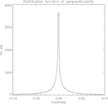
Figure 7. Distribution function for the cosine of the angle between  and
and  for test PDFI solution for AR 11158 at 2011.02.14_23:35–23:47.
Download figure:
Standard image High-resolution imageFourth, the iterative technique is sensitive to noisy input data in  . For example, if we compute a solution to
  using unmasked magnetic field time derivatives and then try to find an electric field contribution that attempts to make
  and
and  perpendicular, the iterative technique can diverge, rather than converge. For this reason, we strongly recommend using masking for the magnetic field time derivative arrays on input to ptdsolve_ss, if the iterative method will then be used to compute the "ideal" contribution.
Finally, we note again that once the solutions for ψ and ∂ψ/∂r are obtained after exiting relax_psi_3d_ss, the resulting contribution from  to
to  is evaluated at the staggered grid locations. This has the advantage of producing a curl-free contribution to
  , but at the cost of losing the direct connection to the angle between
  and
and  , since the vectors are no longer colocated. To evaluate the angle between
  and
and  , the electric fields must once again be interpolated to the CO grid before this comparison can be done. Subroutine angle_be_ss can be used to interpolate electric field components to the CO grid and then evaluate the cosine of the angle between the
  and
and  vectors on the CO grid.
3.9.3. Implementing the Doppler Electric Field Contribution
Given the existence of subroutine relax_psi_3d_ss, the evaluation of Equations (19)–(20) is fairly straightforward, given the input LOS unit vector information, the magnetic field arrays (as input on the COE grid), and the Doppler velocity, also on the COE grid. The Doppler electric field contribution is computed by subroutine e_doppler_ss.
Once all the terms in Equation (20) have been evaluated, subroutine relax_psi_3d_ss is called, and then the gradient of the resulting scalar potential is evaluated.
A few remarks are in order on the resulting electric field contribution. First, in weak-field regions, the behavior of the  unit vector can be very noisy, if the underlying magnetic field is noisy. For this reason, we find much better results if the Doppler velocity and the magnetic field components are multiplied by strong-field masks on input to subroutine e_doppler_ss.
Second, if the region on the Sun being studied is significantly away from disk center, we sometimes find strong contamination of the Doppler velocity from Evershed flows, which then can result in spurious Doppler electric field contributions near LOS PILs at the edges of sunspots.
We have written an alternative subroutine to compute Doppler electric fields based on a different concept, subroutine e_doppler_rpils_ss,
which uses the locations of radial and LOS PILs to try to eliminate these artifacts. Early tests of the effectiveness and accuracy of this subroutine were inconclusive, but it is available for experimentation in the software library.
For now, we retain the original version of e_doppler_ss as the default version, in spite of the above-mentioned defects, as it seems to work well near disk center and behaves correctly for the ANMHD test case described in KFW14 (see also Section 9.2).
3.9.4. Computing the FLCT Contribution
The subroutine that computes the FLCT contribution to the PDFI electric field is e_flct_ss.
The input data for computing the source terms for Equation (24) are the  electric field contributions located on the PE and TE grids, along with interpolated values of Br and
  . We find that it is frequently useful to multiply the Br and
  input arrays by the strong-field mask to reduce the role of noise in the weak magnetic field regions. The divergence on the right-hand side of Equation (24) is then evaluated from the input data onto the CO grid using subroutine divh_co_ss. The Poisson equation for ψF is then solved on the CO grid, but with the Poisson equation domain boundaries defined to be halfway between the edges of the CO and COE grids:
  ,
,  ,
,  , and
, and  . Applying a zero normal-gradient boundary condition at this boundary then allows us to compute ghost zone values for ψF along the edges of the COE grid, resulting in the output scalar potential being defined on the COE grid. Because the Poisson equation boundary is staggered relative to the variables on the corners or vertices, we use the staggered grid version for FISHPACK, subroutine HSTSSP in subroutinee_flct_ss. Once ψF has been computed, the electric field components are computed on the TE and PE grids by taking
  using subroutine gradh_co_ss.
3.9.5. Computing the Ideal Contribution to the PDFI Electric Field
The calculation of the "ideal" contribution to the PDFI electric field is computed by subroutine e_ideal_ss.
On input, the values of Bθ, Bϕ, and Br are provided on the COE grid. Input values of  ,
,  , and
, and  are also provided on their staggered grid locations. The horizontal components of
  are then interpolated to CO grid locations using subroutine interp_eh_ss. To reduce the impact of noise from the weak-field regions, we strongly recommend multiplying the input magnetic field arrays by the strong-field mask array MCOE when calling e_ideal_ss. Next, the hard work for computing the ideal contribution to PDFI is handled by subroutine relax_psi_3d_ss, described earlier in Section 3.9.2, which returns the scalar potential ψI and its radial derivative ∂ψI/∂r, both computed on the COE grid. Finally, the electric field contribution
  is computed on the staggered grid locations by calling subroutine gradh_co_ss for the horizontal components and using the array −∂ψI/∂r for the radial component.
3.10. Poynting Flux and Helicity Injection from PDFI Solutions
Once the PDFI electric field has been computed, there are a number of other useful quantities that can be computed with it, including the radial component of the Poynting flux, as well as the contribution function to the relative helicity injection rate.
These quantities are computed by the subroutines sr_ss and hm_ss.
The subroutine sr_ss takes as input the horizontal components of both the electric field and magnetic field in their staggered grid locations on the TE and PE grids and computes the radial component of the Poynting flux at cell centers (the CE grid). While most of the PDFI_SS software assumes that electric fields are computed as  , in units of G km s−1, subroutine sr_ss assumes that the input electric fields do not include the factor of c and are given in units of V cm−1. To convert from
  in units of G km s−1 to
  in units of V cm−1, one can simply divide by a factor of 1000.
We find that in the weak-field regions, the Poynting flux can be quite unreliable, so we recommend that after output from subroutine sr_ss the resulting Poynting flux array should be multiplied by the strong magnetic field mask for the CE grid, MCE. If the strong-field masks have been used to compute the electric field contributions, then, for consistency, the masks should also be applied on either the input horizontal magnetic fields or the Poynting flux output (which is what we do). The assumed units on output from sr_ss for the Poynting flux are erg cm−2 s−1.
To compute the total magnetic energy input rate from the radial component of the Poynting flux, one can use subroutine srtot_ss
to integrate the radial Poynting flux contribution over area. The output is a single value, computed in units of erg s−1.
The subroutine hm_ss is used to compute the contribution function for the relative helicity injection rate. On input, it uses the poloidal potential P computed from the radial component of the magnetic field using subroutine ptdsolve_ss and the horizontal components of  from the PDFI solution. We typically compute P using arrays of Br that are multiplied by the strong-field mask MCE before ptdsolve_ss is called, so that the vector potential for the potential magnetic field
  does not contain contributions from the weak-field regions. The vector potential
  is computed from P using subroutine curl_psi_rhat_ce_ss within hm_ss. Values of
  and
and  components are then interpolated to the CE grid, and then the quantity
  is computed on the CE grid. The input units for the horizontal electric field are assumed to be in units of V cm−1, and the units for P are assumed to be G km2. The output array is computed in units of Mx2 cm−2 s−1.
One can integrate the contribution function to get a total relative helicity injection rate by calling subroutine hmtot_ss using the output from hm_ss as input. The output is a single value, given in units of Mx2 s−1.
3.11. Putting It All Together: Subroutine pdfi_wrapper4jsoc_ss
The preceding parts of this section have described in detail how the HMI input data are transposed, interpolated, and then used to compute the various contributions to the PDFI electric field, and how that can then be used to create maps of the Poynting flux and the contribution function for the relative helicity injection rate. We have written a subroutine in the PDFI_SS library, pdfi_wrapper4jsoc_ss, that combines all of these pieces together. The SDO JSOC calls this subroutine to compute the electric field and related variables to create the CGEM data series that is distributed by the JSOC. The subroutine is also useful, in that it can serve as a template for a customized calculation of the electric field, allowing a user to eliminate unwanted terms, experiment with various masking strategies for input data, or experiment with new electric field contributions.
The list of major tasks performed by pdfi_wrapper4jsoc_ss, along with the subroutines used for these tasks, is given in order below:
- 1.Transpose the 18 input arrays from longitude–latitude order to colatitude–longitude (theta-phi) order (brll2tp_ss, bhll2tp_ss).
- 2.Convert Doppler velocities from m s−1 to km s−1 and change sign convention to positive for upflows.
- 3.Compute strong-field mask arrays for staggered grid locations from arrays of input magnetic field arrays on the COE grid (find_mask_ss, fix_mask_ss).
- 4.Interpolate input data to staggered grid locations (interp_data_ss, interp_var_ss).
- 5.Compute
 arrays at colatitude edges and cell centers (sinthta_ss).
 - 6.Compute, , and P, T, ∂P/∂r (ptdsolve_ss).
- 7.Compute PTD electric field contribution (e_ptd_ss).
- 8.Compute Doppler electric field contribution (e_doppler_ss, relax_psi_3d_ss).
- 9.Compute FLCT electric field contribution (e_flct_ss).
- 10.Compute ideal electric field contribution (e_ideal_ss, relax_psi_3d_ss).
- 11.Add all four contributions for, convert units to V cm−1.
- 12.Compute radial derivatives of horizontal components of electric field (dehdr_ss).
- 13.Compute Poynting flux and its area integral (sr_ss, srtot_ss).
- 14.Compute contribution function for helicity injection and its area integral (hm_ss, hmtot_ss).
- 15.Transpose all output arrays to longitude–latitude array order (bhyeetp2ll_ss,bryeetp2ll_ss, ehyeetp2ll_ss, eryeetp2ll_ss).
- 16.Return as calling arguments the staggered grid arrays of all three magnetic field components, all three electric field components, the radial derivative of the horizontal electric field components, the radial component of the Poynting flux, the relative helicity injection contribution function, the energy input rate into the upper atmosphere, and the relative helicity injection rate. Note that for the radial electric field component, we output both the total radial electric field and the purely inductive component. The inductive component is used when computing the horizontal components of the curl of, whereas the total radial electric field would be used for the evaluation of, e.g., × , or for evaluating the angle between and (subroutine angle_be_ss). The strong-field mask arrays for the COE, CO, CE, TE, and PE grids are also returned. All returned arrays are oriented in longitude–latitude index order.


The input data sets to and the output data sets from pdfi_wrapper4jsoc_ss are archived and publicly available through the SDO data center with the series names cgem.pdfi_input and cgem.pdfi_output, respectively. They can be directly accessed through the SDO JSOC website http://jsoc.stanford.edu, as are all SDO/HMI and AIA data, or through a variety of other means, including the Solarsoft IDL packages or the SunPy Python package. Users are referred to the SDO data analysis guides for data query and retrieval methods, such as http://jsoc.stanford.edu/How_toget_data.html and https://www.lmsal.com/sdouserguide.html. Each record in these two data series can be uniquely identified via two keywords, CGEMNUM and T_REC, which indicates the CGEM identification number and the nominal observation time, respectively. The CGEMNUM is currently defined to be identical to the NOAA AR number when the CGEM region coincides with a single named active region, and 100,000 plus the SHARP number (Bobra et al. 2014), when the CGEM region consists of multiple active regions or no named active regions. For cgem.pdfi_output, the nominal T_REC is designated at 06, 18, 30, 42, and 54 minutes after the hour. For example, users can find a pair of input records for AR 11158 at the beginning of 2011 February 15 with cgem.pdfi_input[11158][2011.02.15_00:00-2011.02.15_00:12], which includes vector magnetic field, the FLCT velocity field, the Doppler velocity, and the local unit normal vectors. The corresponding PDFI output can be found with cgem.pdfi_output[11158]. The processing necessary to prepare the input data (cgem.pdfi_input) is described in Section 4.
3.12. Errors in Electric Field Inversions
There is currently no formal way for deriving errors in the electric fields within the PDFI_SS software. The fact that the electric field solutions are derived from solutions of elliptic equations means that any magnetic field or Doppler velocity errors result in nonlocalized errors in the resulting electric fields, making analytic error propagation studies difficult. The effects of random errors in the magnetic field measurements and how these propagate into the PDFI electric field inversions in HMI data have been studied by Kazachenko et al. (2015) and Lumme et al. (2019). In Kazachenko et al. (2015), given estimated errors in the radial (30 G) and the two horizontal components (100 G) of the magnetic field determined from the width of distribution functions in the weak-field regions of NOAA AR 11158, this resulted in estimated relative errors of 15%–20% in the three electric field components at a given pixel location for a given pair of AR magnetograms. These results were derived by applying Monte Carlo techniques. Lumme et al. (2019) performed a more detailed error analysis on the PDFI electric fields that was focused primarily on global quantities such as the spatially and/or temporally integrated Poynting flux and helicity injection rate contribution functions. They showed that spatial averaging and temporal integration resulted in significantly lower relative errors than one obtained for individual pixel values for a pair of magnetograms.
Neither of these studies addresses another source of error, the systematic effects to the velocity and magnetic field signals that are due to incomplete corrections for the daily orbital motion of the SDO spacecraft around Earth. These effects appear to generate a false temporal signal at the first few harmonics of the orbital frequency in the magnetic and velocity signals. A false temporal signal in the magnetic field will generate a false electric field through Faraday's law. These systematic errors in the observed quantities from orbital artifacts are characterized by Hoeksema et al. (2014) and Schuck et al. (2016). Schuck et al. (2016) provide a suggested correction for the Doppler velocity that appears to remove much of the artificial temporal signal, but as of yet, no similar correction for the magnetic field components is available. While these systematic errors can affect the electric field solutions over several-hour timescales, short-term variations are small, and the work of Lumme et al. (2019) indicates that they do not greatly affect the time evolution on longer timescales. Nevertheless, the results of the PDFI_SS electric field solutions would be improved if these artifacts could be removed.
3.13. Interpolation of Input Data to Other Resolutions
It is possible that the user may wish to obtain electric field solutions at a different resolution than the 003 resolution provided by the JSOC upstream processing (described in Section 4). One might be tempted to simply interpolate the output electric field results to a different resolution, but doing so will generally destroy the adherence of the solutions to Faraday's law (an exception to this rule is the flux-preserving "downsampling" subroutines, described in Section 5.1, but these only work for certain specified cases to decrease the resolution). We have found that if one wants electric field inversions with an arbitrary change of the resolution, the best solution is to interpolate the input data to the desired resolution and then compute the solutions from scratch from, e.g., subroutine pdfi_wrapper4jsoc_ss.
The interpolation technique we have used for this process is the ninth-order B-spline, a subset of interpolation solutions described by Thevenaz et al. (2000). The low-level source code for this interpolation procedure was written by coauthor Dave Bercik, inspired by Thevenaz et al. (2000) and the accompanying C source code at http://bigwww.epfl.ch/thevenaz/interpolation/. It is implemented in subroutine bspline_ss.
To interpolate a single one of the 18 input data arrays to a different resolution (either coarser or finer), one can use subroutine interp_hmidata_ll,
where the original and desired array dimensions can be specified. In this subroutine, the degree of the B-spline can be specified, but we recommend setting degree to 9. To interpolate the entire 18-level stack of arrays, input as a 3D array, interpolated to a new 18-level 3D array, one can use subroutine interp_hmidata_3d_ll.
This subroutine assumes degree=9. The latter two subroutines assume that the domain boundaries a, b, c, and d remain the same in the output interpolated data arrays as those values for the input arrays.
4. Upstream Data Processing Necessary for PDFI_SS
Before the PDFI_SS software can be run, the full-disk HMI data must be processed into a form where PDFI_SS can use the data. Basically, five procedures are necessary to get the data into a suitable form: (1) Estimate the full-disk Doppler velocity data "convective blueshift" bias, arising because hot upwelling plasma contributes more to the observed intensity than cooler downflowing plasma. (2) The data surrounding an AR of interest must be isolated from the full-disk data and tracked with a rotation rate defined by the center of the AR and mapped into a corotating reference frame. (3) The azimuth angles of pixels' transverse magnetic fields are smoothed in time by flipping any ambiguity choices that produce large, short-lived azimuth changes ("top hats" in the time series of changes in azimuth)—and then the resulting magnetic field, Doppler, and LOS unit vector data are mapped onto a Plate Carrée grid. (4) Successive radial field magnetograms are then used to estimate apparent horizontal motions using the FLCT algorithm. (5) We add a ribbon of data surrounding each of the input data arrays that is set to zero. We find that this "zero padding" improves the quality of the electric field inversions. The source code that performs these tasks can be viewed at http://jsoc2.stanford.edu/cvs/JSOC/proj/cgem/prep/apps/. We now describe these five procedures in more detail.
4.1. Doppler Velocity Correction for Convective Blueshift
The Doppler velocity calibration software that computes the convective blueshift (Welsch et al. 2013) was initially written in FORTRAN by coauthor Brian Welsch and then modified by coauthor Xudong Sun to be called from an HMI module written in C. The module uses full-disk vector magnetograms and Doppler data as input and estimates a "bias" that we later subtract from the Doppler shift measurement. Additional output includes both LOS and radial PIL masks for the LOS magnetic field Bℓ and the radial field Br. The source code for this module can be seen by clicking on the "view" link at http://jsoc.stanford.edu/cvs/JSOC/proj/cgem/prep/apps/doppcal_estimate.f90. We have chosen to work with the Doppler data derived from the full spectral inversion rather than the traditional Doppler data derived from the LOS field pipeline, following the recommendation of the HMI Team. We have performed a comparison between the "vector Doppler" and "LOS Doppler" data. The comparison was done in a cutout that tracked NOAA AR 11158 in full-disk Doppler velocity maps, and it revealed that the two types of raw uncalibrated Doppler maps have systematic differences, with median difference oscillating in phase with the radial velocity of the SDO spacecraft. The removal of the convective blueshift using the method of Welsch et al. (2013) reduces the median difference between the two velocities significantly, particularly in strong-field pixels ( ). Subsequent tests of the impact of the differences between Doppler velocities from the two different data sets on the calculation of the integrated Poynting flux and helicity injection rate showed only a modest difference. We conclude that while there are differences in the results using the two different data sets, our processing reduces these differences, and there is not a substantial difference in the final results.
Once the convective blueshift has been computed, it is used to correct the Doppler velocity measurements during the step described in Section 4.3 below.
4.2. Active Region Extraction
This module extracts a series of AR vector field patches in native coordinates from full-disk data, with constant center latitude (rounded to the nearest pixel), and tracks them at a constant rotation rate. These patches are given a unique "CGEM number" as an identifier and are used as input for the subsequent modules.
4.3. Azimuth Correction and Remapping
This module takes a series of AR patches from Section 4.2; flips ambiguity choices that create large, transient changes in azimuth (see Welsch et al. 2013 for a detailed description); corrects the Doppler velocity with the bias computed in Section 4.1, computes the LOS unit vector; and maps these quantities onto a Plate Carrée (uniformly spaced in longitude and latitude) coordinate system with a pixel spacing of 0.03 heliographic degrees (coinciding closely with the HMI pixel size near disk center). We remove differential rotation based on the fit of Snodgrass (1984), remove the spacecraft velocity, and then correct for the Doppler bias computed from Section 4.1.
4.4. FLCT Horizontal Velocity Estimate
We currently use the local correlation tracking code FLCT (Fisher & Welsch 2008) to estimate horizontal flow velocities, which are then used to compute the noninductive contribution to the horizontal electric field described in Sections 2.3 and 3.9.4. The original idea for local correlation tracking was first described by November & Simon (1988).
The basic idea of the FLCT code is to link small changes in two images taken at two closely spaced times to a 2D flow velocity that moves features in the first image toward the corresponding features in the second image. To compute the "optical flow" velocity at a given pixel location, both images are multiplied by a windowing function, assumed to be a Gaussian of width σFLCT, centered at that given pixel location, to de-emphasize parts of the two images that are far away from the given location. The cross-correlation function of the resulting subimages is computed using Fourier transform techniques, and the location of the peak of the cross-correlation function is found to subpixel accuracy. The difference between the location of the peak and the original pixel location is assigned to be the distance of the pixel shift (in both horizontal directions), and this shift, divided by the time difference between images, is identified with the horizontal flow velocity at that pixel. This procedure is then repeated for all pixel locations in the two images. To compensate for noisy data in the images, the algorithm allows one to select a threshold parameter thr. If the average image value has an absolute value less than thr, no velocity is computed, and a mask value for that pixel is set to zero, to indicate that no value was computed. The velocity itself is then set to zero as well at that pixel. The code also allows the user to filter the images with a low-pass filter before computing the cross-correlation function, if there is a large-degree small-scale noise.
The FLCT algorithm as originally conceived was described in Welsch et al. (2004), with major improvements to the algorithm described in Fisher & Welsch (2008). Since the publication of that article, coauthors Fisher and Welsch have made a number of improvements to the algorithm and the code to increase the accuracy and speed of FLCT. The developer site for the FLCT code is a fossil repository, located at http://cgem.ssl.berkeley.edu/cgi-bin/cgem/FLCT/index. The latest version can always be downloaded there. We have also published a recent snapshot of the FLCT software from the above repository as an archive on Zenodo (Fisher & Welsch 2020).
First, the original C code as described in Fisher & Welsch (2008) was written as a stand-alone executable, intended to be used while running in an IDL session. To read in the image data, and to write out the resulting velocity fields, the information was communicated with IDL using disk I/O. While this works fine for an IDL session, it is inefficient and does not allow the FLCT method to be easily incorporated into other software. Therefore, the current version of FLCT has been rewritten as a library of functions, easily callable from C, FORTRAN, or Python programs. There is still also a stand-alone FLCT executable that has the same user interface as the original version, but this stand-alone code now consists mainly of I/O tasks and calls functions from the FLCT library to perform the main computation. The construction of the library was done in consultation with coauthors Erkka Lumme and Xudong Sun to make sure it could be used from the ELECTRICIT (Lumme et al. 2017, 2019) Python software, from the JSOC's HMI software, and from other FORTRAN test programs.
Second, the FLCT algorithm was rewritten so that the means of the subimages described above are subtracted from the subimages before the cross-correlation function was computed. We found that this resulted in more accurate results.
Third, while the FLCT algorithm as written strictly only applies in Cartesian coordinates, Welsch et al. (2009) described in an appendix of that article how data on a spherical surface can be mapped into a conformal Mercator projection. FLCT can then be run in this projection, and once the velocities are derived, they can be scaled and mapped back onto the spherical surface. We have now modified the FLCT code so that if the input images are given on a Plate Carrée grid, the code itself handles the mapping to the Mercator projection, runs the FLCT algorithm to find the velocities on the Mercator map, and then rescales and remaps the data back to the Plate Carrée grid.
Fourth, we have we performed a study of biases in the calculation of velocities using the FLCT code. A number of published studies have shown that FLCT tends to underestimate flow velocities in cases where the flow velocities are known. Two especially insightful articles on this topic are Freed et al. (2016) and Löptien et al. (2016). The appendix of Freed et al. (2016) quantifies this behavior as a function of FLCT input parameters. Our own study identifies a likely reason for the systematic velocity underestimates, in that the Gaussian windowing function at the heart of the algorithm is centered at the same pixel location in both images, even though the second image has been slightly shifted. We have developed an experimental technique to correct for this bias, which is an input option to the FLCT library functions.
Further details regarding these changes can be viewed in the README file in the latest FLCT distribution, along with documentation files in the doc folder within the distribution. A more complete discussion of the updated FLCT code will be described in a future article.
To compute the FLCT flow velocities in the Plate Carrée data for input to PDFI_SS, for each time, we use pairs of images of Br that are one time step behind and one time step ahead of the current time. So, for the nominal HMI cadence of 12 minutes, the images are 24 minutes apart. The parameter σFLCT is chosen to be 5 pixels. The value of the threshold thr is set to 200 G. We also have chosen not to apply any low-pass filtering of the images in the FLCT code, as we find we get better results overall. For now, we have not implemented the experimental bias correction, but we may apply it in the future.
4.5. Zero Padding the Input Data
We have found that the properties of the electric field solutions are improved by adding a region of "padding" around the input data, in which a ribbon of data with a width of approximately 50–60 pixels is added to each of the four boundaries, with the values of the padded data for all 18 input arrays set to zero. The exact width for each padded region varies slightly, such that the resulting values of m and n are each divisible by 12. This property of the resulting data arrays facilitates the use of the electric field data by the CGEM magnetofrictional model of Cheung & DeRosa (2012), because this property of m and n makes it easier to set up computational runs that use many processors.
Adding the padding is done as the last step before defining the input data for the electric field inversions, and it is performed as part of the HMI magnetic pipeline. To mimic the padding operation within the PDFI_SS library, we have written several FORTRAN subroutines that do the same thing as the JSOC padding process. The subroutine pad_int_gen_ss
takes as input the unpadded values of m and n and "first-guess" values of the amounts of latitude and longitude padding, mpad0 and npad0, and computes output values of m and n and also outputs the exact amounts of padding that will be applied along each of the four boundaries, such that the output values of m and n are divisible by 12.
The adjusted values of a, b, c, and d are computed from the original values of a, b, c, and d, plus the four padding amounts returned by pad_int_gen_ss, by subroutine pad_abcd_as_ss. The padded arrays themselves can then have their interiors filled with the original, unpadded input data, by calling subroutine add_padding_as_ss.
In the test_wrapper.f test program (see Section 9.1), which mimics the call of pdfi_wrapper4jsoc_ss from the JSOC software, these three padding subroutines are called to mimic the same padding procedure performed by the JSOC software. The trial padding values mpad0 and npad0 are set to 50 pixels.
5. Other Applications of the PDFI_SS Electric Field Software
Beyond the calculation of the PDFI electric field solutions in ARs, described in Sections 3 and 4, there are a number of other uses for electric field solutions that use the PDFI_SS library. These can be summarized as (1) curl-free electric field solutions, useful for boundary condition matching; (2) "nudging" electric field solutions for both one- and three-component data-driving in numerical simulations; (3) global (4π sr) PTD electric field solutions; and (4) evaluation of the curl of  , useful for checking electric field distributions for their fidelity in the solution of Faraday's law. These topics will be addressed in this section of the article.
5.1. Curl-free Electric Field Solutions for Boundary Condition Matching
One of the important components of the CGEM project is an electric-field-based Surface Flux Transport Model (SFTM), developed by coauthors DeRosa and Cheung, the details of which will be described in a future publication. A summary can be found in the CGEM final report at http://cgem.ssl.berkeley.edu. The SFTM computes the global horizontal electric field in spherical coordinates based on differential rotation and meridional flows acting on the radial component of the magnetic field, along with a term that describes the dispersal of magnetic flux by supergranular motions. The electric field in the two horizontal directions is then used to evolve the radial magnetic field at the photosphere. The SFTM is used in regions of the Sun for which no PDFI electric fields have been computed, mainly outside of ARs. Where PDFI solutions are computed with PDFI_SS, the model inserts the PDFI solutions into the global domain and evolves Br by using the PDFI solutions, rather than the SFTM solutions. There are two complications to doing this: first, the SFTM generally uses a coarser grid than is used by the PDFI solutions, and second, there will generally be a solution mismatch at the boundary between the PDFI_SS domain and the global SFTM model. Such a mismatch, if not corrected, results in a large, spurious curl of  at the boundaries, which will then result in a spurious evolution of Br at the boundaries or "seams" where the PDFI electric fields are inserted. We now describe how we cope with these two complications.
In general, the SFTM is run with considerably coarser resolution than the 003 resolution computed by default with, e.g., pdfi_wrapper4jsoc_ss in PDFI_SS. Before the PDFI_SS solutions can be inserted into the SFTM model, both solutions must have the same grid resolution. Our approach is to perform a flux-preserving "downsampling" of the higher-resolution electric field results to the same grid resolution that is used by the SFTM. This must be done in such a way that the magnetic flux evolution in the coarser grid is physically consistent with that in the finer grid.
Our solution is to define "macropixels" for the coarser grid in terms of the fine grid, such that there is a whole integer number of fine grid edges fitting within the macropixel edges, in both horizontal directions, and that the line integral of the electric field around the edges of a macropixel is equal to the line integral of the electric field along those fine grid pixels that touch the macropixel boundary. This condition is illustrated schematically in Figure 8.
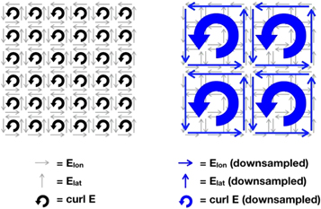
Figure 8. Illustration of downsampling from the high-resolution grid to a coarser resolution grid that is used by the SFTM, where the "circulation" symbol  represents the curl of
  as calculated by taking the line integral of Elon and Elat around the corresponding cell boundary. The electric field on the boundaries of the macropixels is defined such that the line integral of
  is the same as that from the high-resolution grid, and the evolution of
  is consistent between the coarse grid and the high-resolution grid.
Download figure:
Standard image High-resolution imageThe downsampling, considering only horizontal components of the electric field, can be accomplished with subroutine downsample_ss
when using colatitude–longitude array orientation, or subroutine downsample_ll
when using longitude–latitude array orientation, which is the relevant case for the SFTM model. Once downsample_ll has been called, then the coarse-resolution PDFI_SS horizontal electric fields can be inserted into the SFTM model results.
For completeness, we have also written two additional subroutines, downsample3d_ss and downsample3d_ll, which downsample not only the horizontal components of the electric field but also the radial component Er and the radial derivatives of the horizontal components of the electric field. This additional information is needed to create a downsampled three-component electric field that can be used to compute all three components of Faraday's law in the coarser grid in a way that is consistent with the solutions on the original finer grid.
Now we discuss the problem of the mismatch between electric fields in the SFTM and the PDFI solutions, once the latter have been downsampled to the same grid resolution in SFTM. The idea is to add a solution to the PDFI results that has zero curl, but which then matches the SFTM results at the PDFI domain boundaries.
For a curl-free electric field with specified values of the tangential electric field on its boundaries,  obeys the Laplace equation

where the tangential component of the horizontal electric field on the boundaries is related to  by Equation (13). It thus follows that the Neumann boundary conditions needed by the FISHPACK subroutine HSTSSP are given by

for the n points along the north and south boundaries at θ = a and θ = b, respectively, and

for the m points along the left and right boundaries at ϕ = c and ϕ = d, respectively. Once the Laplace equation for  is solved with these boundary conditions, the horizontal components of the electric field within the domain are evaluated by taking minus the curl of
  . These operations are performed by subroutine e_laplace_ss
for arrays in colatitude–longitude orientation and by e_laplace_ll,
where the input electric field components at the boundaries and the output electric fields within the domain are computed in longitude–latitude orientation. The latter case is the one relevant to SFTM, which uses longitude–latitude orientation exclusively.
In the SFTM model, the electric field components at the boundaries on input to these subroutines in Equations (79) and (80) are defined by the difference between the initial SFTM electric field values and the downsampled PDFI electric field values at the boundary locations.
Another useful application of our curl-free electric field solutions is to match boundary conditions assumed in computational models for the solar atmosphere. The PDFI electric field solutions computed by subroutine pdfi_wrapper4jsoc_ss can have nonzero electric field components parallel to the domain boundaries, originating from the contributions from gradients in the scalar potentials. If a computational model requires that the electric field parallel to the boundary is zero, and if the radial magnetic field data are flux balanced, then subroutines e_laplace_ss or e_laplace_ll can be used to compute a curl-free electric field solution that exactly matches the PDFI solution for the tangential component of  on the boundary. That solution can then be subtracted from the PDFI solution, yielding solutions for
  that have zero tangential electric field on the boundaries but still obey all three components of Faraday's law.
5.2. Nudging Electric Field Solutions
Imagine that we have a computational model for the temporal evolution of  in a volume, with the lower boundary surface of the volume coinciding with the photosphere, where we have evaluated Br at the centers of cells in a Plate Carrée grid, and for which we have computed electric field solutions on the edges or rails that surround the cells, using PDFI_SS solutions. The HMI data and the electric field solutions together define a time sequence of magnetic field and electric field solutions that are consistent with one another, at least in terms of Faraday's law. However, the computational model will in general be based on an additional set of physical or mathematical assumptions that can contain far more constraints on how
  behaves in the model. Given some initial condition for
  at t = 0 that matches Br at the photosphere, is there any guarantee that the model's evolution for
  will be consistent with how the HMI magnetic field behaves at the photosphere? In general, the answer to this is no. Given that, sooner or later, the computational model will "go off the rails" as compared to how the observed magnetic field changes over time, what can we do to "nudge" the model to get back on track?
In PDFI_SS, we have developed a series of subroutines that are designed to compute a nudging electric field, in effect giving the computational model a "kick" to make its evolution behave more consistently with the observed magnetic field data. The idea is to use the mismatch between the computational model and the data to compute an electric field that is designed to return the model's magnetic field evolution to match the photospheric magnetic field evolution.
To illustrate this in the simplest way, we consider the computational model to be the spherical version of the magnetofrictional coronal model developed by Cheung & DeRosa (2012). In this model, the observed values of the horizontal components of the magnetic field are not used, and the model is constrained to match the observed evolution of Br at the centers of the photospheric cells, i.e., on the CE grid at the photosphere:

where  . We can use the PTD approximation to compute
  , where

and  obeys the 2D Poisson Equation (9), with the source term equal to the left-hand side of Equation (81). The boundary conditions assumed are the same as those employed in determining
  in subroutine ptdsolve_ss (Section 3.9.1).
A useful way to think about this is to imagine what happens over a single time step Δt taken by the model, assuming that both the target and model magnetic field values are equal at time t:
The vector quantity  is the electric field that must be added to the model's electric field to return Br to its observed value at time t + Δt.
Depending on the details of the computational model, such a nudging step could be taken within the model's own time-advancing algorithm, or alternatively, if the error is small, it can just be added to the model's electric field on output and applied to the calculation of Br for the next time step evolution. The latter case is how the nudging electric field is used within CGEM's spherical magnetofrictional model.
We must add an additional comment on the use of nudging when using electric fields determined from PDFI solutions, as described in Section 3, to drive numerical models. The procedure described in that section recommends using strong-field masks for computing solutions for the electric field. From the perspective of deriving electric fields from the data that are physically meaningful in the presence of magnetic field noise, this is the correct thing to do. However, using these electric fields to drive a numerical model without also using nudging can result in inconsistencies when particular regions of the domain move from being within the strong-field mask region to being in the weak-field region, as time evolves: a given pixel initially within the strong-field region that has a nonzero curl of  will suddenly have zero curl, meaning that the magnetic field at that point will no longer evolve forward in time if only the PDFI solutions of Section 3 are used to drive the model. The use of an additional nudging electric field step, with no strong-field masks applied, will then allow regions of the domain that move between strong-field and weak-field regions to evolve in a way that is consistent with the magnetic field data in both regions. This is how the CGEM magnetofrictional model uses nudging electric fields to address this particular problem.
The nudging electric field in Equation (81) is formally just the horizontal components of the PTD (inductive) electric field from  . It can be computed with subroutine enudge_ss
for input Br error terms in Equation (83), and with outputs Eθ and Eϕ. If the Br error term is oriented in longitude–latitude array order, one can use subroutine enudge_ll
to compute the corresponding components Elon and Elat in longitude–latitude array order.
Another useful application of enudge_ll is within the CGEM SFTM for handling the magnetic field evolution of ARs rotating onto the disk from the east limb of the Sun. The magnetic field observations, if incorporated directly into the SFTM, have unwanted impacts on global magnetic flux balance and other distortions due to the extreme viewing angle. Once the magnetic structure of the rotating AR becomes clearer a couple of days after the AR has rotated onto the disk, the nudging software can be used to reconstruct an artificial but physically reasonable evolution, by using as input to enudge_ll the term on the left-hand side of Equation (81) equal to the difference of the magnetic field 2 days after rotating onto the disk and an initial δBr of 0. The value of Δt in Equation (81) is then set to 2 days. This allows the AR to grow in a natural way within the SFTM without having the unwanted global impacts on the SFTM solution. At that point, the PDFI_SS solutions can begin to be inserted directly into the SFTM as described in Section 5.1.
The concept of nudging can be generalized to include the calculation of all three components of  , in response to evolution in a computational model that computes all three components of
  , instead of just the evolution of Br(t). The same general concept is used: differences between a model's temporal evolution of
  versus a "target" observed evolution can be used to derive corrective values for all three components of
  using the PTD solutions. The primary difference is that in the latter case the electric field components are computed on all the edges (rails) in a 3D layer of voxels bisected by the photosphere, in contrast with the 2D case, in which the horizontal electric fields are computed along the edges surrounding the photospheric face with Br computed on the CE grid. The subroutine enudge3d_ss
can be used to compute the electric fields on all the edges of the voxels, given source term time derivatives for Br, Bθ, and Bϕ and the radial thickness of the voxels. This subroutine assumes that all arrays are in colatitude–longitude order.
5.3. Global PTD (Nudging) Solutions for E
The emphasis of most of the software in PDFI_SS is for spherical wedge domains that subtend only a subset of the full spherical domain. However, for completeness, we have written some electric field software for the global domain (4π sr), including PTD solutions that could also be used for computing nudging solutions in a global domain. This software takes advantage of the special case of "global" boundary conditions available in some of the FISHPACK Helmholtz/Poisson equation subroutines, plus some additional constraints to be applied at the north and south poles in PDFI_SS subroutines. A good discussion of the "global" boundary conditions at the poles can be found in the description of the FISHPACK subroutine PWSSSP in Swarztrauber & Sweet (1975).
The global versions of enudge_ss and enudge_ll, which compute horizontal electric field components from a global distribution of  , are computed by subroutines enudge_gl_ss, and enudge_gl_ll,
for arrays oriented in colatitude–longitude and longitude–latitude order, respectively. Note that with  defined on the CE grid, there are no values of Br defined at the north or south poles. On the other hand, the output arrays of the azimuthal or longitudinal component of the electric field are defined at the poles. Note, however, that physical considerations demand that this component of
  must be zero at the poles, or else the behavior of Br would become singular. The colatitudinal (or latitudinal) component of
  is not defined at the poles. The global solutions for the poloidal potential
  within these two subroutines do not include ghost zones, in contrast to the spherical wedge solutions.
While localized spherical wedge solutions can have a flux imbalance, the global solutions must be flux balanced, to avoid a monopole term in Br or  . Any existing monopole term in the input data is removed before the electric fields are computed. The subroutines fluxbal_ss and fluxbal_ll are used to compute a corrected input field that is flux balanced. The flux balance is corrected in such a way that the locations of preexisting PILs are not moved. The algorithm can be summarized as follows: The positive and negative magnetic fluxes within the domain are summed separately. Whichever polarity is the minority polarity then has the flux in each of its constituent pixels enhanced by a constant relative factor such that the total net radial flux is zero. This is similar to a technique proposed by Yeates (2017), except that in the latter case both polarity regions are adjusted.
In an analogy with the subroutine enudge3d_ss, we can also compute global PTD solutions for all three components of  , given the time derivatives
  ,
,  , and
, and  given on a global, staggered grid. The electric field components are computed on all the edges (rails) of a global set of spherical voxels, similar to the geometry assumed in enudge3d_ss. The solutions are computed by subroutines enudge3d_gl_ss and enudge3d_gl_ll,
for arrays oriented in colatitude–longitude and longitude–latitude order, respectively. The poloidal and toroidal potentials are solved using the "global" FISHPACK boundary conditions mentioned earlier.
There are a number of specific considerations for the north and south poles and the left and right boundaries that must be mentioned. First, the toroidal potential  is defined at the north and south poles. Physically,
  is related to
  at the poles through the Poisson Equation (10), so we need to evaluate the radial current density at the poles. We estimate this quantity by using Ampere's law for
  along the highest latitudes and then dividing by the area subtended by this small disk to estimate
  at the poles. Similarly, we can use periodic boundary conditions for
  to evaluate
  at the left and right boundaries in ϕ. Second, the quantity
  can be defined at the north and south poles, but its value has no effect on the calculation of electric fields from Faraday's law, because the amount of magnetic flux across the θ faces at the poles is zero. Therefore, we assume that
  is zero at the north and south poles, for simplicity. Internal to these subroutines, there are no ghost zones used in the solutions for the poloidal or toroidal potentials.
5.4. Evaluating the Curl of Electric Field Solutions
In order to test the accuracy with which electric field solutions obey Faraday's law, we need to be able to calculate the curl of  . Here we describe a number of subroutines we have written to do this.
One simple and common example is taking the radial component of the curl of the horizontal components of  . Given arrays of Eθ and Eϕ on the PE and TE grids, respectively, subroutine curlehr_ss
will compute  evaluated on the CE grid. This can be compared directly to
  , the radial time derivative of Br (they should be equal and opposite). This subroutine assumes that the arrays are all in colatitude–longitude order.
There are several approaches to computing the curl of  for all three components. If the components of
  are computed on all the rails of a layer of voxels, subroutines curle3d_ss and curle3d_ll
can compute all three components of the curl of  . The quantities returned by these subroutines are actually minus the curl of
  , so they can be compared directly with the time derivative of the three components of the magnetic field and should be equal. It is important that the radial component of
  contain only the inductive contribution to Er. The subroutine curle3d_ss assumes that arrays are in colatitude–longitude order, while curle3d_ll assumes that arrays are in longitude–latitude order. Both of these subroutines can handle either spherical wedge electric field solutions or global electric field solutions.
If one is dealing strictly with electric fields defined at the photosphere, and not in a layer of spherical voxels bisected by the photosphere, there is a different approach that can be used. First, if radial derivatives of the horizontal electric field components have been computed at the photosphere, as is the case when using, e.g., subroutine pdfi_wrapper4jsoc_ss, or when downloading the electric field solutions from the JSOC, one can use subroutine curle3dphot_ss to compute all three components of the curl of  , evaluated at the photosphere. If using quantities downloaded from the JSOC, you will need to (1) transpose the arrays from longitude–latitude to colatitude–longitude array order, (2) convert the units of the radial and horizontal E-fields from V cm−1 to G km s−1 by multiplying by 1000, and (3) convert the units of ∂Eθ/∂r and ∂Eϕ/∂r from V cm−2 to G s−1 by multiplying by 108. It is essential that Er include only the inductive contribution to Er when evaluating the curl. The three components returned by the subroutine are actually minus the curl of
  , so they can be compared directly with the time derivatives of the three magnetic field components.
If the radial derivatives of Eθ and Eϕ are not available, they can be computed with subroutine dehdr_ss,
which uses as input the solutions for the poloidal potential and its radial derivative, as returned from, e.g., ptdsolve_ss.
6. A Potential Magnetic Field Model for Spherical Subdomains with PDFI_SS
For many reasons, it is useful to compute solutions for potential (current-free) magnetic field models in a 3D domain that is consistent with the domain we use for our electric field solutions at the photosphere. Because of our need for these solutions in spherical coordinates for the CGEM project, we include the ability to compute them within the PDFI_SS library. We now discuss the equations for a potential magnetic field model using the same PTD formalism we use to compute the inductive electric field solution at the photosphere.
The electric current density,  , can be derived from the magnetic field,
  , by taking its curl:

We can then substitute the decomposition for  in terms the poloidal and toroidal potentials P and T, using Equation (5), yielding

Focusing for the moment on the middle term on the right-hand side of Equation (85), we note that the net contributions to the curl from horizontal derivatives of  are zero, but there are contributions to the curl of
  from radial derivatives (see Equations (1) and (2)). Evaluating these contributions explicitly yields

Using this result, the expression for  becomes

The first two terms on the right-hand side of Equation (87) represent the horizontal components of the current density  , and the last term represents the radial component of the current density.
For a current-free magnetic field distribution, both the horizontal and radial contributions to  must be zero. Although a number of solutions to this condition involving both P and T are possible, we choose a particularly simple one, namely,

and

Thus, the magnetic field solution is determined entirely by the poloidal potential P, which obeys Equation (88). Note that this equation is not Laplace's equation, in contrast to the case in Cartesian coordinates, where the poloidal potential for a current-free field does obey Laplace's equation (Appendix A of Fisher et al. 2010). We call Equation (88) "Bercik's equation," since to our knowledge it was first derived by coauthor Dave Bercik. This solution will also be a potential magnetic field solution, since a magnetic field distribution with no currents can also be expressed as the gradient of a scalar potential.
It is useful to compare our formulation for the potential magnetic field in terms of P with the similar PTD formulation of Backus (1986) in spherical coordinates. He defines a poloidal potential that we will call  here, but which differs from our P by a factor of r:
  . Backus (1986) shows in Section 4.4 of his article that for a potential magnetic field,
  , i.e.,
  obeys the Laplace equation. Substituting P/r for
  , one finds that P obeys Equation (88), showing that the two PTD formulations for a potential magnetic field are consistent.
Deriving the potential magnetic field distribution from the poloidal potential P has this useful property: if one needs to know either the scalar potential or the vector potential, both are easy to derive from P, whereas converting directly from the scalar potential to the vector potential, or vice versa, can be cumbersome.
Getting the vector potential from P is particularly straightforward: when T = 0, Equation (6) results in

where  denotes the vector potential for the potential magnetic field.
To derive the scalar potential, we first note that the first term in Bercik's equation,  , is equal to −Br. Since the left-hand side of Bercik's equation must be zero, it follows that
Note also from Equation (5) that with T = 0, the horizontal components of  are given by the horizontal gradient of ∂P/∂r. Therefore, all three components of
  can be expressed as the gradient of ∂P/∂r, meaning that the scalar potential Ψ is given by

where we use the conventional definition for the scalar potential Ψ,  . In contrast to the poloidal potential P, Ψ does obey the Laplace equation, as can be seen by setting
  when using
  .
.
The volume domain over which we will find a solution for P will be defined at the bottom by the photospheric boundary at r = R⊙ and will extend up to a radial height of an assumed "source surface" (r = RSS), where the horizontal components of the magnetic field will go to zero. The side walls of the volume will coincide with the same colatitude and longitude boundaries we use for the electric field solutions, θ = a, θ = b, ϕ = c, and ϕ = d. At the photospheric surface, the radial component of the magnetic field will be defined by the observed photospheric radial field. For boundary conditions on the north and south side walls (θ = a and θ = b, respectively) we assume homogeneous Neumann (zero-gradient) boundary conditions for P. For the left and right side walls (ϕ = c and ϕ = d, respectively), we provide two possible boundary conditions: (1) periodic boundary conditions in P, or (2) homogeneous Neumann boundary conditions in P. The side-wall boundary conditions are tantamount to defining the behavior of the vector potential at the boundaries.
In contrast to most spherical potential field models, our solutions use a finite-difference methodology, rather than the more commonly used spherical harmonic decomposition. The spherical harmonic decomposition method is not well suited to high-resolution data, such as those from HMI, and would require the spherical harmonic number ℓ to be several thousand to resolve the 360 km pixels that HMI provides.
Other existing techniques for potential field models in spherical coordinates that do not use spherical harmonic decomposition include the potential field model of Appendix B in van Ballegooijen et al. (2000), the FDIPS finite-difference code (Tóth et al. 2011), the method described by Jiang & Feng (2012), the Green's function approach of Sadykov & Zimovets (2014), and the finite-difference model of Yeates (2018). The FDIPS code uses an iterative approach that applies a Krylov technique, the method of Jiang & Feng (2012) uses a combination of spectral derivatives in the azimuthal direction along with the BLKTRI subroutine from FISHPACK for handling the other two dimensions, and the method of Sadykov & Zimovets (2014) derives a Green's function for the Laplace equation in a portion of the sphere and then integrates this with the observed radial field on the photosphere. Our own technique, described below in detail, resembles that of Jiang & Feng (2012), except that instead of using spectral derivatives in the azimuthal direction, we use second-order-accurate finite differences in azimuth. The finite-difference code of Yeates (2018) also appears to be very similar to our approach, employing the poloidal potential P. Yeates (2018) assumes that grid points in r are distributed logarithmically, rather than linearly.
The FISHPACK library has a capability, through the subroutine BLKTRI, for solving general second-order elliptic finite-difference equations in two dimensions, when they can be expressed in a block-triadiagonal form. This turns out to be the key for deriving a 3D potential field solution using the poloidal potential P in a computationally efficient manner. By Fourier transforming the finite-difference contribution to the horizontal Laplacian from the azimuthal term, the 3D potential field problem can be converted to a series of n 2D finite-difference equations, each of which can then be solved with BLKTRI. Here n is the number of cells in the azimuthal (longitude) direction.
6.1. The Solution for the Poloidal Potential P
The broad outline of the procedure for finding the poloidal potential P is as follows: (1) convert the continuum version of Bercik's Equation (88) to a second-order-accurate finite-difference equation for P; (2) convert the finite-difference version of the azimuthal second derivative term in the horizontal Laplacian to an eigenvalue problem, by Fourier transforming the second-order finite-difference contribution in the azimuth (longitude) direction; (3) derive a 2D finite-difference expression as a function of colatitude and radius for the amplitude of each Fourier mode, with each mode obeying specified boundary conditions in r and θ; (4) solve each one of these resulting 2D elliptic problems using the BLKTRI subroutine in FISHPACK, and (5) inverse transform the resulting solution back to a function in 3D space.
These tasks are all performed within subroutine scrbpot_ss,
which returns the solution P as a 3D array. We now describe these steps in detail.
6.1.1. The Continuum Equation for P and Defining the Finite-difference Grid
The model is based on a solution for P in a 3D domain, where P obeys Bercik's Equation (88). We first multiply Equation (88) by r2 and can then write the resulting equation as

where we have decomposed the left-hand side of the equation into three operators acting on the poloidal potential P. Using Equation (37) for  , we can write these operators as


and

The locations where P is defined must be consistent with the 2D staggered grid locations defined in Section 3.4. In three dimensions, we have 3D voxels instead of 2D cells. P must be defined on the radial faces of the voxels and in the center of these faces, to be consistent with the location of P on the CE grid at the surface of the photosphere. We will therefore denote the indices for P with i +  as the θ index, j +
  as the ϕ index, and q for the index of radial faces, in keeping with the index notation described in Section 3.7. We will place the source surface as the last radial face of the active part of the domain. If there are p + 1 radial faces in the r-direction, it means that the radial spacing Δr is given by

where p is the number of voxels between R⊙ and RSS. The dimension of P is therefore (m, n, p + 1) in the θ-, ϕ-, and r-directions, respectively. Figure 9 shows a diagram of a voxel in this 3D grid.

Figure 9. Schematic diagram showing one voxel of our staggered 3D spherical grid for the potential field solutions, based on the Yee grid concept. The poloidal potential P lies at radial face centers of each voxel. Br is located at radial face centers, Bθ at θ face centers, and Bϕ at ϕ face centers.
Download figure:
Standard image High-resolution imageIn this section of the article, where describing finite-difference expressions, we assume index ranges that start at 0 and go to p in the radial direction for P, from  to m −
  in the θ-direction, and from
  to n −
  in the ϕ-direction. But keep in mind that when examining these expressions in the source code we have used default index ranges in FORTRAN, where the first index starts from 1.
6.1.2. Fourier Transform P in Azimuth and Derive Finite-difference Equations for Each Fourier Mode
We now make the assumption that the solution for P can be separated into a product of eigenfunctions in the azimuthal direction multiplied by coefficients that are a function of colatitude θ and radius r, where each eigenfunction can be enumerated by a wavenumber index, j'.
Let

where  are a series of orthogonal basis functions in ϕ' and
  are the amplitudes for each one of these n basis functions. Here, the azimuthal variable ϕ' has its range normalized to be from 0 to 2π, instead of from c to d:

The expression for Lϕ operating on P when using second-order-accurate finite differences in ϕ becomes, for each Fourier mode j',
Here, the factor of (2π/(d−c))2 accounts for the scaling of the second derivative between ϕ and ϕ', and the quantity Δϕ'2 is the square of the corresponding spacing between grid points in ϕ' (Δϕ' = 2π/n).
If we let the basis functions  be complex exponentials

(or sines and cosines over the same range of ϕ'), then it is straightforward to show that the above finite-difference expression becomes
Note that the factors of (2π/(d−c))2 and the expression for Δϕ'2 = (2π/n)2 occuring in Equation (100) result simply in division by Δϕ2 in Equation (102). Equation (102) depends explicitly on wavenumbers k(j'), whose values depend on the details of the Fourier transform implementation. In the limit of low wavenumber, the cosine expression in Equation (102) results in the second derivative term being proportional to −k(j')2, as one would expect, but as the wavenumber increases, the behavior deviates from this, also as one might expect since the finite-difference expression begins to deviate from the spectral derivative result.
The most important point is that the result of applying the Lϕ operator to  is simply multiplication by a factor (the eigenvalue of the operator) times that same function. Since the other two operators Lθ and Lr that define Bercik's equation do not depend on ϕ at all, the result will be a common factor of
  for all three operators, which can then be factored out. Furthermore, since the
  are all orthogonal to each other, the sum of the three operators for the Bercik equation acting on the solution must be zero not only for the entire solution but also for each individual term in the expansion (98). Therefore, for each value of the Fourier mode j', we need to determine only the coefficients
  . When evaluating the finite-difference versions of Lθ and Lr, we will therefore consider their action only on
  .
.
Evaluating Equation (95) using second-order-accurate finite differences, applied to  , we find
for i +  that is not adjacent to the θ = a or θ = b boundaries. For
  , adjacent to the θ = a boundary, the homogeneous Neumann boundary condition on P means that the ghost zone value
  must be equal to
  . Since the expression for the operator that will be input into BLKTRI cannot involve ghost zones, we can make that substitution into the operator equation to eliminate
  and then find
Doing a similar exercise for  , adjacent to the θ = b boundary, after applying the homogeneous Neumann boundary condition we have
For the finite-difference version of the Lr operator Equation (96) acting on  we have
The boundary condition at the last radial point, rp = RSS, is determined by the outer boundary condition that Ψ is a constant we can set to 0, meaning that the radial derivative of  is zero. The ghost zone value,
  , must therefore be equal to
  , which then results in the equation for the operator acting on the last radial point
6.1.3. Getting the Finite-difference Equations into Block Tri-diagonal Form
The finite-difference Equations (102)–(107) for each Fourier mode j' can be written in a block tri-diagonal form, which can then be used as input for the FISHPACK subroutine BLKTRI. The block tri-diagonal form means that for each of the given values of i +  and q the finite-difference expressions for
  involve only points at i −
  , i +
, i +  , and i +
  in the θ-direction and only points at q − 1, q, and q + 1 in the r-direction. Subroutine BLKTRI expects the coefficients for the finite-difference equations to be input through six 1D arrays, am, bm, cm (each dimensioned m), and an, bn, cn (each dimensioned p + 1). The array am specifies the coefficients multiplying
  for each of the m values of i +
  , bm specifies the diagonal coefficient (the one multiplying
  ), and cm specifies the coefficient multiplying
  . These can be found by inspection of Equations (103)–(105). The array bm, the diagonal coefficients, must also include the term from Lϕ multiplying
  in Equation (102). Note that for
  , am = 0, and for
  , cm = 0. The arrays an, bn, cn are the coefficients multiplying
  ,
,  , and
, and  in Equations (106) and (107). Note that at q = p, cn = 0. As described in more detail in Section 6.1.5, at the photospheric level q = 0, the values of an, bn, cn will all be zero.
6.1.4. Fourier Transform Details: Applying Azimuthal Boundary Conditions and Determining Wavenumbers
So far, we have said little about the eigenfunctions  . If we use the standard Fourier transform expansion of complex exponentials, or equivalently pairs of sines and cosines, then the eigenfunctions obey periodic boundary conditions, and the wavenumbers in the expansion assume their conventional values. This is one of the options available in our software. The other expansion we have assumed is the half-wave cosine transform, in which all of the eigenfunctions are cosines and have zero derivative at either end of the ϕ domain. In this case, the homogeneous Neumann boundary condition is achieved, and the range of ϕ' goes from 0 to π instead of from 0 to 2π (in Equation (99)
  ).
).
The choice of boundary conditions in ϕ is made through an input argument bcn, to subroutine scrbpot_ss. Periodic boundary conditions are chosen by setting bcn=0, while homogeneous Neumann boundary conditions are chosen by setting bcn=3. These values correspond with the same boundary condition values used in other FISHPACK subroutines.
In both cases, we have adopted the Fast Fourier Transform (FFT) software that is already included in FISHPACK, called FFTPACK. We make this choice primarily for convenience. The wavenumbers k(j') needed in Equation (102) are computed with subroutine kfft_ss
for the periodic boundary condition case and with subroutine kcost_ss
for the homogeneous Neumann boundary condition case. We find that the overall speed of scrbpot_ss does depend on the choice of boundary condition: the compute time for homogeneous Neumann boundary conditions is roughly twice that for periodic boundary conditions.
6.1.5. Matching the Solution to Observed Br at Photosphere, and Photospheric Boundary Conditions for Fourier Coefficients
At the photospheric layer (q = 0, or r = R⊙) we specify the arrays an, bn, cn so that at the first array elements all three array values are set to 0. This means that at this layer we ignore the radial variation of  and instead will set the horizontal Laplacian (determined by the am, bm, cm arrays) to match the observed values of Br. To do this, we must determine from the observed data what the value of each Fourier coefficient
  is at the photosphere.
The procedure is straightforward. Given the observed photospheric array of Br on the CE grid  , we first solve the horizontal Poisson equation

using FISHPACK subroutine HSTSSP. Once we have the solution, we then Fourier transform the solution in the ϕ-direction. The Fourier transform then results in the values of  . Applying the horizontal Laplacian operator (from arrays am, bm, cm) will result in the Fourier transform of −r2Br at the photosphere,
  . This can be used to specify a 2D source term array expected by BLKTRI, y, which is dimensioned (m, p + 1). For each Fourier mode j', we can set y(0:m-1,0)=
 . All the other values of y for q > 0 are set to 0, consistent with the right-hand side of Bercik's equation being set to 0 for all radial layers above the photosphere. In principle, one should be able to Fourier transform the observed array Br directly and do the same thing, but in practice this produces significant artifacts mainly due to the effects of flux imbalance in the input data. The procedure as described above, on the other hand, appears to be robust and accurate.
6.1.6. Assembling the 3D Solution from BLKTRI
Once the photospheric values  are known for each value of j', we can then perform a loop over j' and call BLKTRI to get the solutions for
  for all the radii from R⊙ to RSS and all the colatitudes between a and b. After each solution is obtained, we store the results in a 3D array dimensioned (m, p + 1, n), which is basically the Fourier transform of P, but stored with the Fourier transform index j' as the last index for the array. We then perform a final loop and both inverse Fourier transform the results back to real space and transpose the index order such that the result is the 3D array
  . The output array P is dimensioned (m, n, p + 1).
6.1.7. Testing the Accuracy of scrbpot_ss
We have written a subroutine to test the accuracy with which the finite-difference version of Bercik's equation is satisfied: subroutine berciktest_ss,
which computes minus the horizontal Laplacian of P and the radial second derivative of P and provides these two quantities as output variables. We find that these two computed quantities agree closely with one another, with an accuracy that approaches roundoff error. Having this subroutine available was extremely useful in developing and debugging the code in subroutine scrbpot_ss.
6.2. Computing the Vector Potential and Magnetic Field Components from P
We first make some general comments about the properties of the solution for P determined from subroutine scrbpot_ss: (1) for well-resolved solutions, the resulting 3D array P can be huge; (2) if the input radial magnetic field at the photosphere has a net flux imbalance, the P solution will not reflect the flux imbalance (i.e., it is consistent with a net radial magnetic flux of zero); and (3) the solution for P includes no ghost zones. Part of the reason for not constructing ghost zones is because the array is already so large. In addition, we find that where ghost zones are needed to evaluate curls or gradients, we can add them on an as-needed, layer-by-layer basis. All of the subroutines we discuss here perform this operation internally when necessary.
While the solution for P computed by scrbpot_ss has no net radial flux, we feel that it is important for the potential field solutions to include a net flux when the user desires it. We therefore include a subroutine, mflux_ss, which can be used to compute the net radial flux from the input radial magnetic field data. The resulting net radial flux is then used to augment the solution for P to result in a potential magnetic field solution that is consistent with the data. The output from mflux_ss is a single value of the net radial flux ΦM over the photospheric domain defined by the values of R⊙, a, b, c, and d.
The vector potential  within the 3D volume can be computed in a straightforward way from P and from ΦM. The radial component of
  is zero, so only the horizontal components of
  are computed.
The vector potential  is computed by subroutine ahpot_ss, using P and ΦM on input, and on output computing the two components of
  , Aθ and Aϕ, each of which are 3D arrays of dimension (m, n + 1, p + 1) and (m + 1, n, p + 1), respectively. The quantity Aθ is computed along radial faces of the voxels, on the PE (phi-edge) grid locations in the horizontal directions, and Aϕ is also on radial faces but on the TE (theta-edge) grid locations in the horizontal directions. To compute
  , there is an outer loop over the radial index q. Then, for each radial layer, ghost zones are added to P that correspond to the boundary conditions assumed at the θ and ϕ edges of the domain. Then,
  is computed for that given radius using subroutine curl_psi_rhat_ce_ss, populating the Aθ and Aϕ arrays at that radius. After that, an additional term is added to Aϕ:

where B0 = Φm/Aphot and θi are the colatitude values of the cell edges in the θ-direction. Here, the photospheric area of the domain is given by

After adding  to Aϕ, the vector potential preserves any radial net flux that is included with the observed radial magnetic field data. If zero net radial flux is desired, one can simply set ΦM = 0 on input to ahpot_ss.
Once the vector potential has been computed with ahpot_ss, it can be used to compute all three components of the potential magnetic field by using subroutine curlahpot_ss.
The outputs from this subroutine are Bθ, Bϕ, and Br, with each component of  computed at the corresponding face centers of each voxel: Bθ is computed at the θ face centers, Bϕ is computed at the ϕ face centers, and Br is computed at radial face centers. Bθ is computed from radial derivatives of Aϕ, Bϕ from radial derivatives of Aθ, and Br using subroutine curlh_ce_ss acting on Aθ and Aϕ. The dimensions of these arrays are (m + 1, n, p) for Bθ, (m, n + 1, p) for Bϕ, and (m, n, p + 1) for Br.
We also have the ability to compute the magnetic field components directly from P and ΦM, if desired, with subroutines brpot_ss and bhpot_ss.
Subroutine brpot_ss does an outer loop over radial index q. For each radial layer, ghost zones are added to P to make the solution consistent with the applied boundary conditions on the θ and ϕ edges of the domain. Then, the pair of subroutines curl_psi_rhat_ce and curlh_ce_ss are called in succession to compute the horizontal Laplacian of P, which then results in the values of Br within that radial layer. An additional term is then added to the solution,  , where, as before, B0 = ΦM/Aphot, to account for any net radial magnetic flux. The radial magnetic field component lies in the center of radial voxel faces.
Subroutine bhpot_ss does an outer loop over the radial index q, and first differences P between two adjacent levels in r to evaluate ∂P/∂r, after ghost zones have been added to each of the two layers. This derivative is evaluated at voxel centers in radius and also in θ and ϕ. Then, both Bθ and Bϕ are evaluated by using subroutine gradh_ce_ss to take the horizontal gradient of ∂P/∂r. Here, a net radial magnetic flux plays no role in the result and so is ignored. The output arrays Bθ and Bϕ are computed at θ and ϕ face centers, respectively.
The array dimensions of Bθ, Bϕ, and Br when computed by brpot_ss and bhpot_ss are identical to those computed by curlahpot_ss. The values of all three magnetic field components computed using the two different methods agree with each other to a high degree of accuracy, with an error level just slightly worse than roundoff error.
One defect of the staggered grid formalism used here is that the horizontal magnetic field components computed with the model at the lowest radial layer do not lie on the photosphere, where we have the magnetic field measurements, but instead lie half a voxel above the photosphere. We would like to compare and contrast horizontal magnetic field components from the data with their potential field counterparts lying on the photosphere. Fortunately, we can use the finite-difference form of Bercik's equation to infer the photospheric values of the horizontal magnetic field components. Equation (91) shows that
where  would be the ghost zone value for ∂P/∂r just below the photosphere. We know Br at the photosphere from the data, and from the solution for P, we can difference P to find
  , so we can solve for the ghost zone value below the photosphere:

Once this has been done, we can then interpolate (average) ∂P/∂r between values at  and
and  to get the photospheric value of ∂P/∂r,
Then, the horizontal gradient of this quantity yields the potential field values of Bθ and Bϕ at the photosphere. These operations are carried out by subroutine bhpot_phot_ss.
The subroutine uses the solution P computed by scrbpot_ss and observed photospheric values of Br on input and computes Bθ and Bϕ at the photosphere on output. Bθ lies along the TE grid, and Bϕ lies along the PE grid. These arrays can be compared directly to the staggered grid values of the observed data, for comparisons of the differences and similarities between the observations and what the potential field model predicts. Figures 10–13 show test results of the potential field software, using data from a vector magnetogram of AR 11158 taken on 2011 February 15, 22:47 UT. The values of m, n, and p for this calculation are 632, 654, and 1000, respectively. The value of the assumed source surface was RSS = 2 R⊙. Here, the homogeneous Neumann boundary condition in ϕ was used to compute the solution. On an Apple MacBook Pro (early 2015), with 16 GB of RAM and an SSD disk drive, these solutions can be derived and written to disk on timescales of roughly 10 minutes, using a single processor, with the compute time noticeably shorter for periodic boundary conditions in ϕ as compared to homogeneous Neumann boundary conditions. The compute time is dominated by subroutine scrbpot_ss. Once the solution for P has been obtained, evaluating the magnetic field components takes a small fraction of the total compute time. In the horizontal directions, the angular resolution is close to that of HMI; in the radial direction, Δr is roughly 700 km, about twice the horizontal spacing as that at the photosphere.
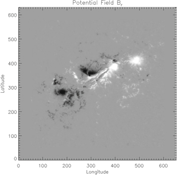
Figure 10. Here we display, in longitude–latitude order, the image of Br from the potential field solution at the photosphere computed from subroutines scrbpot_ss, ahpot_ss, and curlahpot_ss. The vector magnetogram data were taken from HMI data of AR 11158 on 2011 February 15, 22:47 UT. The maximum error between the given observed values of Br and the model values are less than 10−6 G. The linear grayscale range in the figure is from −2000 to 2000 G.
Download figure:
Standard image High-resolution image
Figure 11. Images of Bϕ, both from the observed vector magnetogram data (top) and from the potential field solution at the photosphere (bottom), plotted in longitude–latitude orientation. The potential field solution at the photosphere is computed from subroutines scrbpot_ss and bhpot_phot_ss. The vector magnetogram data were taken from HMI data of AR 11158 on 2011 February 15, 22:47 UT. Note the significant differences between the Bϕ values at the sheared neutral line and the similar behaviors at the sunspots. The linear grayscale range in the figure is from −2000 to 2000 G.
Download figure:
Standard image High-resolution image
Figure 12. Images of Bθ, converted to Blat, both from the observed vector magnetogram data (top) and from the potential field solution at the photosphere (bottom), plotted in longitude–latitude orientation. The potential field solution at the photosphere is computed from subroutines scrbpot_ss and bhpot_phot_ss. The vector magnetogram data were taken from HMI data of AR 11158 on 2011 February 15, 22:47 UT. Note the significant differences between the Blat values at the sheared neutral line and the similar behaviors at the sunspots. The linear grayscale range in the figure is from −2000 to 2000 G.
Download figure:
Standard image High-resolution image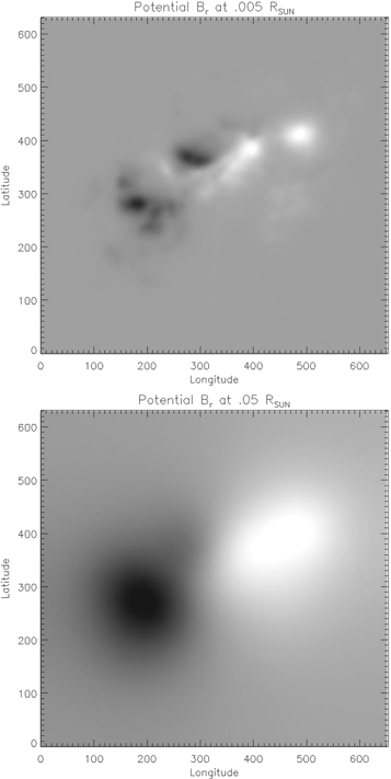
Figure 13. Images of the potential field solution for Br, plotted in longitude–latitude orientation, at distances above the photosphere of 0.5% (top) and 5% of R⊙ (bottom). The potential field solution above the photosphere is computed from subroutines scrbpot_ss, ahpot_ss, and curlahpot_ss. The vector magnetogram data were taken from HMI data of AR 11158 on 2011 February 15, 22:47 UT. The linear grayscale range in the figure is from −1200 to 1200 G for the top image and from −80 to 80 G for the bottom image.
Download figure:
Standard image High-resolution image6.3. Nearly Global Potential Field Source Surface (PFSS) Models
While our potential field software was designed for deriving solutions on AR-sized portions of the Sun, it can also be used for deriving solutions that lie above a very large fraction of the solar disk. First, the range of ϕ can be extended to the entire circumference of the Sun by simply choosing c = 0 and d = 2π and then choosing the periodic boundary condition option in ϕ (bcn=0) when calling scrbpot_ss. Second, we have tested the software by choosing very small values of a and values of b that approach π, with no major ill effects or artifacts near the poles. In particular, we have chosen a and b such that their values differ from 0 and π by only 001 without difficulty. We then compared the morphology of the solutions at various radii computed with the spherical-harmonic-based PFSS model of D. J. Bercik & J. G. Luhmann (2019, in preparation), using moderate numbers for maximum spherical harmonic degree, with solutions from the software in PDFI_SS described here, using compatible resolution for the finite-difference equations presented here. The solutions seemed compatible overall at several different radii between the photosphere and the source surface.
6.4. Using the Potential Field Software to Compute Electric Field Solutions in the Coronal Volume
If, instead of specifying the radial magnetic field at the photosphere, one specifies the partial time derivative of the radial magnetic field at the photosphere, subroutine scrbpot_ss will find  instead of P. In that case, if one then calls subroutine ahpot_ss with
  as input, the output will be the electric field components cEθ and cEϕ (both with a minus sign) throughout the coronal volume. These are the electric fields that correspond to the time derivative of the corresponding potential magnetic fields in the volume. Calling subroutine curlahpot_ss will then compute the time derivative of all the magnetic field components in the volume defined by the potential field software. If homogeneous Neumann boundary conditions in ϕ are chosen (bcn=3), these solutions will be compatible with the PTD solution for
  at the photosphere computed from ptdsolve_ss and e_ptd_ss, apart from the minus sign. It then becomes possible to perform detailed investigations of how the electric field corresponding to the changing potential magnetic field distributions behaves in the coronal volume.
Electric fields computed in this way appear to be generally consistent with one of the contributions to the electric field  identified with the changing potential magnetic field in the analysis of Schuck & Antiochos (2019). They identify that electric field as coming from a solenoidal contribution, denoted
  , plus that from the gradient of a scalar potential, denoted
  . The calculation described above will compute a solenoidal (inductive) version of
  . However, looking at trial test cases indicates that along the
  and
and  normal faces of the spherical wedge volume, the component of the electric field normal to these surfaces is not zero, in contrast to the boundary condition (32c) assumed for
  in Schuck & Antiochos (2019). This is true for either bcn=3 or bcn=0, neither of which constrains the behavior of the component of
  normal to the faces. Thus, the PDFI_SS solutions do not appear to be consistent with the assumed boundary conditions for
  in Schuck & Antiochos (2019).
Apart from this, we have not yet pursued any further detailed studies using this possible application of the PDFI_SS potential field software at this time, but simply point out this possibility for future work.
6.5. Computing Energies for the Potential Magnetic Field
Once the 3D distributions of the magnetic fields have been computed, it is straightforward to estimate the energy in the potential magnetic field, by either performing an integral of B2/(8π) over the computational volume or estimating this quantity through a photospheric surface integral, using Gauss's theorem, and ignoring side and top boundaries. We have written three subroutines to provide such estimates. These subroutines are emagpot_ss, emagpot_srf_ss, and emagpot_psi_ss.
Subroutine emagpot_ss takes as input the three 3D arrays Bθ, Bϕ, and Br; interpolates the magnetic field components from voxel faces to the voxel centers; evaluates B2/(8π) at the center of each voxel; and then sums up the magnetic energy density from each individual voxel. The advantage of this subroutine is that no assumptions about side-wall boundary conditions are made; a possible disadvantage is that magnetic field energy outside the volume is not computed and therefore underestimated. Energies are computed in units of ergs.
Subroutine emagpot_srf_ss uses the fact that the volume integral of B2/(8π) can also be written, using Gauss's theorem, as an area integral of  over all the surfaces surrounding the volume, where
  is the outward surface normal vector for each surface. However, the subroutine ignores all the surfaces except the photosphere and simply integrates
  over the photospheric domain. On input, the subroutine takes the photospheric values of Aθ, Aϕ, and the potential field values (not the observed values!) of Bθ and Bϕ as, e.g., computed from bhpot_phot_ss. We find that emagpot_srf_ss tends to overestimate magnetic energies to a modest degree when compared to the results from the volumetric integral computed by emagpot_ss. Most likely this is due to the effects of ignoring all the nonphotospheric surfaces in the area integral.
A third subroutine for computing the magnetic energy is emagpot_psi_ss. Here, the photospheric values of the potential magnetic field Br and the scalar potential Ψ are used on input to compute the magnetic energy by integrating ΨBr/(8π) over the photospheric surface. This equation also results from a use of Gauss's theorem, when  is expressed as minus the gradient of the scalar potential Ψ. With our solutions derived in terms of P, this is less convenient to use than emagpot_srf_ss, since Ψ = −∂P/∂r is normally not evaluated at the photosphere, but half a voxel above it. However, Equation (113) shows a strategy to evaluate Ψ = −∂P/∂r at the photosphere, which is implemented in PDFI_SS by calling subroutine psipot_phot_ss.
We also find that emag_psi_ss tends to overestimate magnetic energies compared to the volumetric integral computed by emagpot_ss, probably for similar reasons to emagpot_srf_ss.
6.6. Transposing Potential Field Solutions from Colatitude–Longitude to Longitude–Latitude Order
The potential magnetic field solutions are computed in colatitude–longitude order for computational purposes within the PDFI_SS software, but for display purposes, as well as other applications that use longitude–latitude array orientation, we want an efficient capability to transform the 3D solutions from colatitude–longitude orientation to longitude–latitude orientation.
We have written several subroutines to perform these transpose operations, ahpottp2ll_ss, bhpottp2ll_ss, and brpottp2ll_ss.
The subroutine ahpottp2ll_ss converts the two components of the vector potential from colatitude–longitude order to longitude–latitude order and also changes the sign from Aθ to Alat. The subroutine bhpottp2ll_ss does the same operation on the horizonal components of the potential magnetic field, also changing the sign of Bθ when converting to Blat. The subroutine brpottp2ll_ss transposes the radial magnetic field array, Br. It can also be used to transpose the poloidal potential itself, P.
Since this is a very memory-intensive operation, in the potential field documentation file Potential-Fields-Spherical.txt located in the fossil repository http://cgem.ssl.berkeley.edu/cgi-bin/cgem/PDFI_SS in the doc folder, there is a discussion of how one can use a combination of C and FORTRAN pointers to perform the transpose operations "in place" if desired, which uses significantly less memory. No change to the existing source code for the transpose subroutines in the PDFI_SS library is necessary to do this; this memory-sharing operation is done entirely in the calling program. This same principle is also outlined in Section 9.4, which describes a test program for doing these transpose operations.
6.7. Computing Potential Magnetic Fields Using Bh
Welsch & Fisher (2016) showed an alternative method for deriving potential magnetic fields from vector magnetogram data, where, instead of matching Br at the photosphere, one could match  as measured from the data. They found that these solutions could result in quite different values of Br at the photosphere as compared to the observations, just as potential field models based on Br can have horizontal magnetic fields that differ considerably from the observed values (see, e.g., Figures 11 and 12). Welsch & Fisher (2016) found that potential field solutions matching
  can have substantially smaller magnetic energies than those matching Br. We have implemented a technique for finding potential field solutions that match
  using much of the same potential field framework described above. We now outline this technique, which is included in the PDFI_SS software.
We first note that relating the poloidal potential P to  in a way that can use BLKTRI is not as straightforward as it was for relating P to Br. However, if we solve for the scalar potential Ψ instead of P, then much of the mathematical and numerical framework we use in scrbpot_ss can be adapted to solve for Ψ.
Writing  and then taking the horizontal divergence of
  at the photosphere, we have

where in the volume above the photosphere Ψ obeys the Laplace equation
Equation (114) is of exactly the same form as Equation (108), but involving Ψ and  instead of P and Br. Equation (115) has a somewhat different radial term than does Bercik's Equation (88), but it is compatible with the use of BLKTRI. The source surface boundary condition at r = RSS will differ between P and Ψ. We now describe the details of how the equation for Ψ is solved, particularly where the details differ from those in Section 6.1.
6.7.1. Finite-difference Expressions for the Laplace Equation for Ψ and the Solution Procedure
Our strategy for solving the Laplace Equation (115) is identical to that for solving Bercik's equation. We will convert the azimuthal, colatitude, and radial derivatives to finite differences and then Fourier transform the equations in the azimuthal direction and derive finite-difference equations for the amplitude of each Fourier mode as a function of θ and r. Using the same notation of Section 6.1.2, the operators Lϕ and Lθ, when converted to finite-difference form, will be identical to the operators in Section 6.1.2, where we also assume homogeneous Neumann boundary conditions at θ = a and θ = b.
As in Section 6.1.2, we write the solution Ψ as

where  is the amplitude of the coefficient of
  as a function of colatitude and radius indices. The actions of the Lϕ and Lθ operators on
  are identical to those in Section 6.1.2.
Since the Lr operator differs from that in Section 6.1.2, we write down the result:
for values of q that are in the interior of the problem. For the outermost radial position q = p, we want to impose the boundary condition that  as
as  , so that
  . This means we have a ghost zone value of
  . Since BLKTRI does not use ghost zones, we make this substitution into Equation (117), resulting in
From Equations (117) and (118) we can easily determine the values of the arrays an, bn, and cn for radial positions above the photosphere in subroutine BLKTRI.
As in Section 6.1.5, the first (photospheric) values of the an, bn, and cn arrays are set to zero.
The solution procedure for the finite-difference equations for Ψ is otherwise identical to that described in Section 6.1 for P. Getting the solution for Ψ is carried out by subroutine psipot_ss.
To test the accuracy with which Laplace's equation is obeyed by Ψ, we have written the subroutine laplacetest_ss, which outputs separately the horizontal and radial contributions to the Laplacian. We found that this was useful in debugging psipot_ss.
Finally, there is an issue that the solution to the Laplace equation can contain a spurious artifact in Ψ that is proportional to r−1. The origin of this artifact appears to be an interaction between the source surface boundary condition for Ψ, which essentially sets Ψ = 0 at r = RSS, and the homogeneous Neumann boundary conditions in θ for the k = 0 mode at the photosphere, when BLKTRI is called for this particular mode. This, in effect, allows Ψ at the photosphere to "float," i.e., to have an arbitrary constant added to it. At radii in between the photosphere and source surface, the solution is connected by an r−1 dependence that satisfies the Laplace equation. This solution, while mathematically legitimate, has no physical basis and results in a sometimes large, horizontally uniform radial component Br that must be removed from the solution. We have written a subroutine psi_fix_ss, which evaluates and removes this artifact, by evaluating the Br term at the photosphere and then removing it from the entire solution volume. This subroutine is called just before exiting subroutine psipot_ss. Subroutine psi_fix_ss can also be used to impose an observed nonzero net radial flux to the solution for Ψ, if desired.
6.7.2. Getting the Potential Magnetic Field Components from Ψ: Subroutine bpot_psi_ss
In principle, once Ψ is known, the magnetic field components can be found by simply taking minus the gradient of Ψ. In practice, there is a major challenge to deriving the magnetic field components from Ψ: gradients of Ψ put the magnetic field values in a different location in the grid from where we need it. We now describe how we evaluate the magnetic field components at the grid locations where we need them.
The scalar potential Ψ lies at the centers of the radial faces of our voxels. In the horizontal directions, Ψ lies on the CE grid (see Figure 9). The grid location of Ψ in the horizontal directions is different from the grid locations of the scalar potentials ψ for computing the electric field contributions at the photosphere, where these various scalar potentials all lie on the COE grid. This is why we have used the notation of the uppercase Ψ to distinguish the scalar potential for the potential magnetic field derived from  from the notation of the lowercase ψ contributions to the photospheric electric field.
When we take horizontal gradients of Ψ, the results lie on the θ and ϕ edges of the radial faces, but we need them at midpoints in radius (midway in r between radial faces) at the centers of the horizontal faces of the voxels in θ and ϕ). Similarly, when we take the radial component of the gradient of Ψ to get Br, it is evaluated at midpoints in r within the voxels, but we need Br on radial face centers.
We now describe how we interpolate the horizontal magnetic field components from the θ and ϕ edges of radial faces to the θ and ϕ face centers of our voxels.
If we imagine that we have another set of voxels ("offset voxels") that are offset by  from our grid voxels, then we also imagine that each of our voxels contains the upper half of an offset voxel in the bottom half of our given voxel, and the bottom half of the next highest offset voxel in the top half of our voxel. We want the θ and ϕ magnetic fluxes from our voxel to match the flux from the top half of the lower offset voxel, plus the flux from the bottom half our the upper offset voxel. These considerations result in the following expression for the interpolated horizontal magnetic field components:
and
where we use the fact that the area of the side faces of a voxel are proportional to  if the bottom and top radial faces of the voxel are located at rq and rq+1.
Now that we have values of Bθ and Bϕ interpolated to horizontal face centers, we can evaluate  at voxel centers, using subroutine divh_ce_ss, where the result projected onto the horizontal directions lies on the CE grid. We can then use the constraint
  to derive the radial derivative of r2Br:

Since Br evaluated from  is also colocated with
  , we can use Equation (121) to extrapolate Br to the upper and lower radial faces, where we want the values. The evaluation of
  and the extrapolation to radial faces are done within subroutine br_voxels3d_ss.
All of these tasks are accomplished within subroutine bpot_psi_ss.
If a nonzero net radial flux is desired for the potential field, one can specify its value in the input variable mflux in the call to bpot_psi_ss.
If one wants to compute a solution for Ψ itself that is consistent with an imposed net radial flux, one can call subroutine psi_fix_ss with a nonzero value of the net radial flux mflux. Doing this is advisable if using Ψ to compute magnetic energies with subroutine emagpot_psi_ss.
6.7.3. Testing Potential Field Models that Use Bh at Photosphere
How can we characterize the accuracy of solutions to the potential field models that use photospheric values of  ? The interpolation and extrapolation steps described in Section 6.7.2 will introduce some amount of error into the magnetic field solutions, as compared to the solutions based on Br, where these steps are not needed. Our objective here is to provide a method for estimating errors in the solution obtained from
  .
.
The test described here is based on the following procedure: (1) First, obtain the potential field solution that matches observed photospheric values of Br using subroutines scrbpot_ss, ahpot_ss and curlahpot_ss, along with subroutine bhpot_phot_ss to compute the horizontal potential field components at the photosphere. (2) Using the photospheric potential field components Bθ and Bϕ computed from the above, compute the scalar potential Ψ to match  at the photosphere by calling subroutine psipot_ss. (3) Compute the magnetic field components by calling subroutine bpot_psi_ss. (4) Compare the original solutions for Bθ, Bϕ, and Br with those computed from Step 3, and evaluate the discrepancies. Figure 14 shows the recovered values of Br versus the original values of Br from the data, showing an rms difference of ∼18 G. For comparison, the scatter plots of the recovered values of Bθ and Bϕ (not shown) look like straight lines and have much smaller errors. Similarly, the original potential field model based on Br shows errors of ∼10−6 G, in recovered versus observed values of Br, close to roundoff error. Thus, the largest source of error seems to be the interpolation and extrapolation procedures in subroutine bpot_psi_ss that were needed to compute Br at radial face centers. While these errors are visible here, they are smaller than the quoted HMI errors in Br, so we feel that the solutions are accurate enough for many scientific studies.
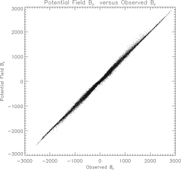
Figure 14. Scatterplot of photospheric values of Br computed from potential field solution derived from  , vs. the observed values of Br. The components of
  used as input were computed from the potential field solution that was based on the observed values of Br. The scatter away from a straight line measures the error introduced by the interpolation/extrapolation procedures needed to get the magnetic field components located in their correct positions on the grid. The rms errors in Br are ∼18 G, smaller than quoted HMI errors for Br.
Download figure:
Standard image High-resolution image6.7.4. Applications of Potential Field Solutions from Bh
Welsch & Fisher (2016) proposed the idea that potential field models derived from vector magnetograms can include observed data from  and Br and proposed composite models where both solutions can be used, with weights for each based on measurement errors for the different components of
  considered separately. Because our potential field software in PDFI_SS includes the ability to compute both solutions, this can be done in a straightforward way.
We also note that Welsch & Fisher (2016) proposed that differences in Br between the observations and the  potential field solutions may provide a diagnostic for the existence of horizontal currents. For AR 11158, we show such a difference image of Br in Figure 15. It is interesting that in the sunspots there is only a slight difference in Br, but there are also large-scale patterns elsewhere in the AR showing a significant difference. This potential field software makes more detailed studies a practical possibility.

Figure 15. Difference between Br computed from the potential field that matches the observed values of  and the observed values of Br, from 2011 February 15, 22:47 UT. Welsch & Fisher (2016) suggest that difference images such as this result from horizontal currents flowing in the solar atmosphere. Using the solutions from subroutines psipot_ss and bpot_psi_ss, these difference images are straightforward to compute. The linear grayscale range used to display this image is −1500 to 1500 G.
Download figure:
Standard image High-resolution image7. Using PDFI_SS to Compute Electric Field Inversions in Cartesian Coordinates
There are times when it makes more sense to compute electric field solutions in Cartesian coordinates rather than in the spherical coordinates assumed in PDFI_SS. How can we adapt the PDFI_SS library for Cartesian coordinates without creating a completely separate version? Our approach to answering this question is to note that, to an excellent approximation, a very small patch near the equator of a very large sphere will be, for all intents and purposes, a Cartesian coordinate system.
Suppose that we want to perform electric field inversions in a Cartesian coordinate system with Nx cells in the x-direction and Ny cells in the y-direction, and that each cell in x has a width of Δx and each cell in y has a width of Δy. The total extent of the domain in the x- and y-directions is thus Lx = NxΔx and Ly = NyΔy. We want to map this domain onto the surface of a large sphere with radius R, with the y range bisected by the equator, at latitude zero (or colatitude of  ). The important point is to make the value of the sine of the colatitude θ for all the cells close to unity, meaning that variations due to spherical geometry are negligible. Specifically, we want the colatitude range b–a to subtend a small angle, ΔΘ, such that
  and
and  are close to unity. Given ΔΘ, we then have

and

Setting RΔΘ = Ly, we obtain

where R is the desired radius of the sphere. Once R is determined, the longitude range d–c can be determined as

If one knows the longitude of the left boundary from solar disk observations and wishes to preserve it, then that value can be assigned to c, and then d can be assigned by adding to c the results of Equation (125). If the value of c is unimportant, we can assign

and

These values of a, b, c, and d, along with R, define the spherical geometry parameters for a Cartesian coordinate system on the surface of a large sphere. The only question is what value to assign for ΔΘ. Our experience has been that setting ΔΘ = 1 × 10⁻⁴ has worked well for most of the cases we have tried. It is small enough that the sine of colatitude is essentially unity, but large enough that roundoff errors in Equations (122) and (123) are not important.
The subroutine car2sph_ss will compute the resulting values of R, a, b, c, and d, given an input value of ΔΘ and input values of Δx and Δy, along with the number of cells in the colatitude and longitude directions, m and n. This subroutine will assign a value of 0 to c. It is important to remember that n and m are the same as Nx and Ny in the above discussion of the Cartesian grid. If ΔΘ is set to 0, then internal to the subroutine a value of 1 × 10⁻⁴ will be used. After output from car2sph_ss, if one wishes to keep an original value of the leftmost longitude to solar disk coordinates, then that value should be added to the values of c and d on output from the subroutine. The variable rsun used in many of the PDFI_SS subroutines should then be assigned to the output value of the variable rsph from the car2sph_ss.
One complication with going from Cartesian to spherical coordinates using this scheme is that the input Cartesian data will be arranged in longitude–latitude index order, whereas most of the mathematical operations in PDFI_SS are performed using colatitude–longitude index order.
If one is performing the entire PDFI electric field solution, and the input data are not yet on the staggered grid, the subroutine pdfi_wrapper4jsoc_ss can be used on the Cartesian input data, since this subroutine expects the input data to be in longitude–latitude order and performs the needed interpolations to the staggered grid locations. If one is performing a more customized calculation, or some other operation using the PDFI_SS software such as potential magnetic field solutions, the user will need to use the transpose and interpolation subroutines described in Section 3.6 to get the data into colatitude–longitude index order on the staggered grid locations.
8. Compiling the PDFI_SS Library, and Linking It to Other Software
In this section of the article, we will first describe the history of the PDFI_SS library development. Then, we will discuss some choices made in writing the FORTRAN source code for PDFI_SS. We will then describe how to compile the library, followed by discussions of how to link the library to other software written in FORTRAN, C/C++, and Python. We will end by describing the use of the legacy PDFI_SS software written in IDL.
8.1. The History of the PDFI_SS Software
The first published study in which time-dependent vector magnetic fields were used to derive electric fields was that of Fisher et al. (2010; earlier, Mikić et al. 1999 described electric field solutions determined from time derivatives of the radial component of  ). In this case, ANMHD magnetoconvection simulation data (Welsch et al. 2007), which had known electric field solutions, were used to create a vector magnetogram data sequence, which could then be analyzed by computing PTD solutions for
  . While there was a broad resemblance between the inverted PTD solutions and the actual electric fields, there were also a number of artifacts. The authors developed an "iterative" technique to compute an additional scalar potential, whose gradient could be added to the PTD solutions to make
  and
and  perpendicular to each other, resulting in a moderately better agreement between the inverted and actual electric fields. A further investigation in that article used a variational approach, to impose a "smallness" constraint to the electric field solutions, which resulted in a poor match with the actual ANMHD electric fields. We subsequently gave up on using the variational approach.
The PTD Poisson equations were solved in Fisher et al. (2010) using a FORTRAN version of the Newton–Krylov technique, originally developed for the first version of RADMHD (Abbett 2007), since the required boundary conditions were inconsistent with the use of FFTs. Solutions obtained with the iterative method, which used repeated solutions of a Poisson equation, were performed in IDL using FFTs.
A great improvement in the accuracy of the electric field inversions of the ANMHD simulations was made in Fisher et al. (2012), in which it was realized that adding information about Doppler shifts, which can be measured, resulted in dramatically better solutions for the electric field. They derived Poisson equations for contributions from both Doppler shifts and horizontal flows derived from Local Correlation Tracking, which were then solved in IDL using FFTs, with the solutions added to the PTD solutions obtained with the Newton–Krylov software.
In 2011–2012, coauthors Maria Kazachenko, Brian Welsch, and George Fisher realized they needed more efficient software for solving the Poisson equations, in which many more types of boundary conditions could be applied, and which would be faster than their existing Newton–Krylov code. They tested several numerical techniques and concluded that the elliptic equation package FISHPACK was ideally suited to these tasks. They proceeded to write a very general executable program in FORTRAN, which could be spawned from IDL, which would read input data, compute the solutions using FISHPACK, and then write the solutions to a file, which could then be read back into the IDL session. This software model for PDFI existed from roughly 2012 through 2015, during which the centered, Cartesian version of the PDFI software was developed. We now refer to this version as PDFI_CC, where "CC" refers to "Cartesian centered." This is the version of the software that was used to perform the research described in Kazachenko et al. (2014, 2015).
Starting in 2013, the above coauthors received funding for the CGEM project (Fisher et al. 2015), in which they proposed to take the existing PDFI software and (1) convert it to spherical coordinates and (2) rewrite it in an efficient computer language that could be run automatically from the SDO JSOC. This process happened in several stages. First, the Cartesian IDL source code had to be converted from Cartesian to spherical coordinates. This process took roughly 6 months and maintained the use of a centered grid. (This version was called PDFI_SC, where "SC" denotes "spherical centered.") In the meantime, by studying MuRAM MHD simulation results obtained from Matthias Rempel at HAO/NCAR, which had turbulent structures at the scale of the grid, the authors realized that the centered grid finite-difference formulation was simply unable to obey Faraday's law accurately when the solutions were so highly structured. They realized they needed to convert their finite-difference equations into a conservative, staggered grid coordinate system. After investigating several different formulations of staggered grid systems, they finally arrived at the system described in Section 3.4.
Once the PDFI_SC version was written and working in IDL, the next step was to convert the IDL code from the spherical centered grid to the spherical-staggered grid scheme. This process occurred during the first half of 2015. By July of 2015, an IDL version of PDFI_SS was operational and had successfully undergone a number of tests.
To deliver the software in a form that could be run automatically at the SDO JSOC, the coauthors knew that the IDL code would have to be converted to FORTRAN, since it relies so heavily on the FISHPACK FORTRAN library. The conversion of the code from IDL to FORTRAN was done during the last half of 2015 and early 2016. Since that time, nearly all development effort has been on the FORTRAN version of the software. The FORTRAN version of PDFI_SS now contains a much broader spectrum of capabilities than the original IDL version did. While we continue to keep the IDL legacy version within the PDFI_SS developer site, we no longer actively maintain the IDL branch of the software. We do find that the existing IDL code, particularly the procedures for performing vector calculus operations, can still be useful when analyzing output from PDFI_SS.
8.2. Comments on PDFI_SS FORTRAN Source Code Choices
There were a number of choices made in how the PDFI_SS FORTRAN code was written. Here we briefly comment on these and discuss the motivations for these choices.
First, the calling arguments for all the subroutines include input and output arrays, as well as other important information provided as single real scalar values or as integers. All quantities defined as arrays have their dimensions defined in terms of integer values passed into the subroutine by the user. Modern FORTRAN allows one to determine array sizes and shapes by querying the attributes of these arrays, potentially reducing the number of necessary calling arguments. However, we found that these advanced features did not work when the PDFI_SS subroutines were invoked from other C and Python software. Thus, we define all array dimensions from other calling arguments in the subroutines.
Second, we have avoided any use of "common-block" variables, or other global parameters or variables, which can obscure the dependencies of output variables on input arguments. All input data are passed explicitly as calling arguments into the FORTRAN subroutines. This constraint eases the ability to use the library from languages other than FORTRAN.
Third, all floating-point operations are performed using 64 bit reals. All reals, either scalars or arrays, are declared as real*8 variables in the source code, a choice that seems to work correctly with all FORTRAN compilers attempted thus far. All integer arguments to PDFI_SS subroutines are assumed to be default integers in FORTRAN, which are 32 bit integers.
Fourth, the source code assumes that all input and output arrays are dimensioned or allocated (and deallocated) by the user in the calling programs. This is essential for the software to be used from languages other than FORTRAN. Thus, very few of the arrays in PDFI_SS are dynamically allocated within the source code. The one exception to this rule are the work arrays needed by FISHPACK subroutines. In this case, for each PDFI_SS subroutine that calls a FISHPACK subroutine, the work array is both allocated and then deallocated within that same subroutine.
Fifth, to facilitate ease of interoperability with C code, character string arguments have been completely avoided in the PDFI_SS software. Character strings have a different representation in memory between FORTRAN and C.
Finally, the FORTRAN syntax is implemented using the older .f suffix for the source code file names, rather than the more modern .f90 suffix. While the latter choice results in more flexible syntax for, e.g., line continuation, the former choice helps enforce 80-character line limits, which makes viewing the source code much easier from the default 80-character width of a terminal window.
8.3. How to Compile the PDFI_SS FORTRAN Library
The first step in compiling PDFI_SS is to download, compile, and install the FISHPACK FORTRAN library. Links for the FISHPACK version 4.1 source code are given in the introduction to Section 3.
After unpacking the tarball, we recommend that you replace the contents of file make.inc in the top folder of the FISHPACK distribution, with the contents of the file fishpackmake.inc located in the doc folder in the PDFI_SS distribution, then replace the file Makefile in the top folder of the FISHPACK distribution with the contents of the file fishpackmake in the doc folder in PDFI_SS, and finally replace the file Makefile in the src folder of the FISHPACK distribution with the contents of the file fishpackmakesrc in the doc folder in PDFI_SS. You may need to edit the file make.inc to (1) make sure that the name of the FORTRAN compiler coincides with the name of the FORTRAN compiler you have. We have specifically included lines for the gfortran and Intel compilers in the Linux part of the make.inc file, and the gfortran compiler for the Mac (Darwin) portion of make.inc. If you are using another compiler, you will need to edit the compiler definition F90 so that it reflects your compiler. (2) Make sure that the options included in defining the FORTRAN compiler also ensure that all reals are set to 64 bit reals. (3) Check that compiler options for compiling position-independent code, needed if FISHPACK will be used for languages other than FORTRAN, are invoked. (4) Edit definitions for make and ar, if they are different from what is defined in this file.
We cannot overemphasize how important it is to invoke the compiler option that all reals are treated as 64 bit reals. If this is not done, the attempted use of FISHPACK with PDFI_SS is doomed to fail, in ways that are not always easy to diagnose.
To compile the FISHPACK library, type "make." Once the FISHPACK library is compiled, you can install it into a location of your choosing by typing "make install" (or "sudo make install" if this requires root priviledge). Alternatively, you will need to remember the exact path to the location of the library file libfishpack.a.
Once FISHPACK has been compiled and installed, we are ready to compile PDFI_SS. As noted earlier, the PDFI_SS software developer site is http://cgem.ssl.berkeley.edu/cgi-bin/cgem/PDFI_SS/index. By clicking on "Login," one can log in as anonymous, and then by clicking on "Files," one should find a blue hexidecimal link, the ID for the latest software release. By clicking on that link, one should then be led to links for tarball or zip archives for the software.
Once the tarball has been downloaded and unpacked, you should see three subfolders: IDL, doc, and fortran. Descend into the fortran folder with a terminal window.
The next step is to open the file "Makefile" with an ASCII text editor, such as vi or emacs. You will most likely need to edit this file before you can compile the library. Currently, the Makefile is set up assuming you will be running on either a Mac or a Linux machine of some kind, and that you have access to a FORTRAN compiler. The file assumes you will have access to either the gnu/gfortran compiler or the Intel compiler, ifort. If you plan to use a different FORTRAN compiler, you will need to edit Makefile to add the name of that compiler and to add compiler options for it that coincide with the meanings of the compiler options for gfortran or ifort.
To compile the PDFI_SS library file, libpdfi_ss.a, type "make." To install the library into a specified location, edit the definition of INSTALLDIR, and then type "make install" (or possibly "sudo make install," if you need root privilege for the specified location). The default value of INSTALLDIR is /usr/local/lib.
8.4. Linking PDFI_SS to Other FORTRAN Programs
Once the PDFI_SS library has been installed, linking to other FORTRAN programs is straightforward. For the gfortran and ifort compilers, linking to the library is invoked with the -lpdfi_ss -lfishpack (in that order) linking commands. If the libraries are not stored in "standard" locations, you may need to specify the location of each library with the -L<dir> directive. Specific examples can be found in the test programs, described in further detail in Section 9.
8.5. Linking to PDFI_SS Subroutines from C/C++
If there are no character string arguments, calling a FORTRAN subroutine from a C function is very straightforward, if one just remembers some basic rules: (1) From C, a FORTRAN subroutine is a function of type void (i.e., the function returns nothing). All input and output are handled through the calling arguments. (2) The name of a FORTRAN subroutine is changed by the FORTRAN compiler ("FORTRAN name mangling"); typically this is done by adding a trailing underscore. This practice is observed by both the gfortran and ifort compilers. In other words, in C, if one wants to call ahpot_ss, the corresponding function name in C is ahpot_ss_. (3) In FORTRAN, all arguments are called by reference, not by value. This means that when calling a FORTRAN subroutine from C, all arguments must be passed by reference, i.e., as pointers. For example, if in a C function calling a FORTRAN subroutine the variables m and n are declared as integers, their pointers &m and &n would be used in the call to the subroutine. (4) FORTRAN is a column-major language. For multidimensional arrays in FORTRAN, the first index always varies in memory the fastest. For example, a 2D array brll, dimensioned (n + 1, m + 1) in FORTRAN, assumed to be in longitude–latitude orientation, is ordered such that we start with the smallest latitude value, increase the longitude index from the smallest to the maximum value, then repeat the process with the next-lowest latitude index value, etc. C is considered to be a row-major language, so that given a 2D array in C, the second index varies the fastest in memory.
From our experience, the easiest way to deal with this possible source of confusion is, first, to stick with using 1D arrays in C of length (n + 1) ∗ (m + 1) using the above example and, second, to make sure that all input 1D arrays are arranged in column-major order before calling the FORTRAN subroutine. On output, we also recommend defining 1D arrays in C, keeping in mind that the output data will be ordered by the FORTRAN subroutine into column-major order. If you need the data arranged in a different order, you will need to do that rearrangement after the subroutine call. Fortunately, 1D arrays in C map neatly onto multidimensional arrays in FORTRAN, provided that one keeps in mind the assumed column-major order. For FORTRAN arrays of three or more dimensions, the same principle works: define an array in C of length equal to the product of the FORTRAN dimensions, and make sure that the first index varies the fastest, followed by the second index, followed by the next index.
The size of default integers in FORTRAN is 32 bits, so the C calling program should be sure to not use 16 bit or 64 bit integers when calling the subroutines. For nearly all systems, a declaration of int in C should be compatible with FORTRAN integer arguments to PDFI_SS subroutines. Similarly, all real variables in PDFI_SS are 64 bit reals, compatible with the double precision (double) declaration in C. The PDFI_SS subroutines assume that the calling program has already allocated memory for both input and output arrays. All memory management for the calling arguments to PDFI_SS subroutines is assumed to be handled by the calling program and is not done within PDFI_SS itself.
We have written as one of our test programs (see Section 9.8) a simple C program that calls the brll2tp_ss subroutine. The program shows explicitly how the input array is constructed and ordered into column-major order before calling the subroutine, and when the output array is printed, one sees that the output array is also arranged in column-major order, using the transposed dimensions.
We strongly recommend defining function prototype statements for any PDFI_SS subroutines you call from a C program (in C99, these statements are required). This reduces the chance of making errors in calling the subroutine from C and can be helpful in debugging the code by warning the user when calling arguments disagree with those of the function prototype. We have written an include file (pdfi_ss.h) that contains the function prototypes in C for all of the user-callable subroutines in PDFI_SS. This file can be included in any C code that calls PDFI_SS FORTRAN suboutines. In our test C program (Section 9.8), our test program C source code includes this file.
There is little difference in calling PDFI_SS subroutines from a C++ program compared to a C program. The same rules about passing arguments (all arguments are passed by reference, i.e., as pointers) apply. The main difference is that (1) in the C++ program you will need to set the lang=C option, and (2) the compiler options for position-independent code must be invoked when compiling PDFI_SS. In our Makefile, we have endeavored to make sure this option is chosen for the gfortran and ifort compilers.
8.6. Linking the PDFI_SS Library into Python
Linking the PDFI_SS library into the Python programming language allows effective use of the software with solar-physics-related open-source Python packages, such as SunPy (Mumford et al. 2015) and astropy (Astropy Collaboration et al. 2013), as well as easy manipulation, analysis, and plotting of the input and output data using the basic Python modules NumPy, SciPy (Jones et al. 2001), and matplotlib (Hunter 2007). The PDFI_SS-Python linking has also been used to implement the PDFI_SS electric field inversion into ELECTRIC field Inversion Toolkit, ELECTRICIT (Lumme et al. 2017, 2019). ELECTRICIT is an easy-to-use Python software toolkit for downloading and processing of SDO/HMI data and inverting the photospheric electric field from the data using a range of state-of-the-art methods.
We have successfully created a working Python interface for several PDFI_SS functions using the F2PY FORTRAN to Python interface generator https://docs.scipy.org/doc/numpy/f2py/, which is a part of the NumPy package. F2PY is compatible with FORTRAN 77/90/95 languages and allows partly automated creation and compilation of Python interfaces for FORTRAN routines and functions. The generator includes several methods of creating the interface, from which we have chosen to use the method based on signature files. The process has the following steps: (1) The F2PY package is used to automatically create a signature file (e.g., pdfi_ss.pyf) from the FORTRAN source code. The signature file specifies the Python wrapping of the PDFI_SS routines of interest (e.g., pdfi_wrapper4jsoc_ss). (2) The automatically created signature file is then modified to ensure working wrapping of the FORTRAN routines (usually only modest changes are required). (3) Finally, F2PY is used to compile an extension module (e.g., pdfi_ss.so) from the modified signature file and FORTRAN source code and/or compiled libraries. The extension module and its functions are then importable and callable in Python (import pdfi_ss, output=pdfi_ss.pdfi_wrapper4jsoc_ss(arg1,arg2,...)).
8.7. Using the Legacy IDL Code for PDFI_SS
We have retained the original IDL procedures that we used in the early phases of the development of the PDFI_SS library, although this software is no longer maintained. We find that the software is sometimes useful in the analysis of magnetic and electric field data generated by the library.
In this version of the software, there is still the need for a FORTRAN executable to solve the PDFI Poisson equations, but this executable is spawned from the IDL code when needed, and nearly all of the computational results apart from the solutions themselves are performed in IDL. The source code for the FORTRAN executable xpoisson is contained within the file poisson_arguments_stag.f and is compiled and installed with the Makefile that is in the IDL folder. The xpoisson executable is a very general wrapper for the FISHPACK subroutines HWSCRT, HSTCRT, HWSSSP, and HSTSSP and allows one to select either Cartesian or spherical coordinates and either centered or staggered grid solutions. The xpoisson executable does extensive error checking on all the input parameters for the FISHPACK subroutines before solving the Helmholtz or Poisson equation. To communicate the input data to xpoisson, and to read the output solutions from xpoisson, the "Simple Data Format" or sdf binary data format is used, and this library must be compiled and installed before xpoisson can be compiled and run.
The sdf library is written in C but is designed to be used from either C or FORTRAN. The objective of the sdf library is to read and write binary files containing both simple variables and large arrays, by calling simple subroutines or functions from FORTRAN or C. It was developed to aid in the debugging of numerical codes, making it easy to output and examine the contents of large arrays. The sdf library also has a set of IDL procedures to read and write sdf files, making this a convenient way of communicating between an IDL session and the FORTRAN executable. Coauthor Fisher developed and maintains the sdf library. The source code for sdf can be downloaded from http://solarmuri.ssl.berkeley.edu/~fisher/public/software/SDF/. Use the latest version. An archive of the latest version of this software at the time this article was published can also be downloaded from Zenodo (Fisher et al. 2020a).
The PDFI_SS IDL source code contains the core abilities to compute the PTD and FLCT terms, the relaxation procedure (needed for the Doppler and ideal contributions) to the PDFI electric field, but lacks much of the additional capabilities of the FORTRAN library. Computing solutions with the IDL code is also much more time-consuming than using the FORTRAN library software. Nevertheless, we sometimes find that the vector calculus procedures, which have nearly the same names as the corresponding FORTRAN subroutines, can be useful in analyzing the results from PDFI_SS solutions.
9. Test Programs Using the PDFI_SS Software
In the course of writing the PDFI_SS library, it was necessary to develop a series of test programs to detect bugs accidentally introduced into PDFI_SS subroutines from code revisions and to test new capabilities as they are being developed. Output from the test programs can then be examined to see whether the results make sense. The test programs are contained within the test-programs folder of the fortran folder of the PDFI_SS distribution.
Most of the test programs need to read in binary data from input files and write out the binary results. All of these input/output data (except for the Python test) are assumed to be written using the Simple Data Format (sdf) format that was introduced in Section 8.7. The names of the needed input files are provided in the document README.txt contained in the test-programs subfolder. Copies of the needed input files can be obtained from http://cgem.ssl.berkeley.edu/~fisher/public/data/test_data_pdfi_ss/, also available as a data set on Zenodo (Fisher 2020). The test programs (aside from the Python test) assume that the input files are located in the test-programs folder mentioned above. For the Python linking test, the input files are assumed to be placed into the python-linking folder within test-programs. We have typically analyzed the output from the test programs using an IDL session, in which we read in all the contents of the output file written by the test program. If all of the IDL procedures from the sdf distribution are in your IDL path, this command is very simple: sdf_read_varlist, 'outputfile', where outputfile is the file name created by the test program. Then, typing "help" in the IDL session will display all of the variables and arrays that were written out. These results can then be studied and analyzed in IDL.
Next, we provide the names of the test programs and their purpose, and then we will describe how to compile the test programs. A detailed description of each test program will then be provided in subsections of this section.
The names of the test program source code files and the purpose of the test program are given in Table 2.
Table 2. Test Program File Name and Purpose
| Source Code | Purpose |
|---|---|
| test_wrapper.f | Test pdfi_wrapper4jsoc_ss |
| test_anmhd.f | Test ANMHD electric field inversions |
| test_bpot.f | Test potential field (from Br) |
| test_bptrans.f | Test 3D transpose of potential field |
| test_psipot.f | Test potential field (from  ) ) |
| test_global.f | Test global PTD solution for 
|
| test_interp.f | Test ninth-order B-spline interpolation |
| test_pdfi_c.c | Test PDFI_SS library function from C |
| python-linking | Test PDFI_SS linking from Python |
Download table as: ASCIITypeset image
To compile the suite of FORTRAN and C test programs, there is a Makefile in the test-programs folder. Edit the Makefile to make sure that the definitions of the FORTRAN and C compilers are consistent with your system. Make sure that the library locations for the sdf and fishpack libraries are correct in the Makefile, and that the PDFI_SS library has been compiled in the overlying fortran folder. Then, typing "make" in a terminal window should compile all the test programs. The test programs can be removed by typing "make clean."
To run the Python test script, first make sure that the NumPy and SciPy packages are installed for the version of Python you plan to use. Edit the Makefile in the python-linking folder to set the version of the Python executable. Then, typing "make" should compile the shared object file pdfi_ss.so. This enables one to then run the script pdfi_wrapper4jsoc_script.py, allowing the FORTRAN subroutines to be called from Python. The names of the needed input data files are given in the README.txt file in this folder. The files themselves are available at the URL referenced above.
We must caution that the test programs test_bpot.f, test_bptrans.f, and test_psipot.f, when compiled as the executables xbpot, xbptrans, and xpsipot, respectively, use huge amounts of memory and create huge output files, and they can take a long time to run, particularly if you have insufficient memory. We recommend running these test programs only on systems with at least 16 GB of memory free and with a solid-state disk.
9.1. test_wrapper.f (Executable xwrapper)
The source code in test_wrapper.f is designed to mimic the JSOC's call to subroutine pdfi_wrapper4jsoc_ss. In a nutshell, it reads in test magnetogram and Doppler data from HMI, along with stored FLCT estimates of horizontal flows, then adds padding to the data in a manner consistent with how this process is done upstream of the PDFI_SS call by the JSOC, and then calls the subroutine pdfi_wrapper4jsoc_ss. The output from the subroutine is written to an output file. The test program also independently computes each of the four electric field contributions and also writes these to the output file, so that a detailed and independent comparison can be made. The program computes and writes to the output file many other diagnostic quantities.
We must caution that the input data used here are taken from a preliminary test data series for NOAA AR 11158 generated several years ago and do not reflect a number of improvements to the data analysis that have occurred since that time. The FLCT flow velocities, in particular, were generated with nonoptimal parameter choices. Nevertheless, since these data are fixed here for the purpose of testing the PDFI_SS code, not the data analysis procedures, we have retained their use in this test program.
The documentation at the front of test_wrapper.f includes a list of the variables from the output file, if read into an IDL session with the procedure sdf_read_varlist. Here, we will discuss only a summary of the overall PDFI_SS electric field results for this particular test case. Particularly important diagnostics one can examine with the output data include comparison of the curl of  with the temporal difference in magnetic field components between the two adjacent vector magnetic field measurements.
One can use quantities in the output file to examine a detailed breakdown of the PDFI solutions into their four contributions, which are computed independently within test_wrapper.f. For further details, see the documentation at the head of the test_wrapper.f source code file.
We end our discussion of test_wrapper.f by displaying in a series of grayscale figures (Figures 16–22) the three magnetic field components for the test data, along with computed PDFI electric field inversions for the three components of  . Both the inductive and total contributions to Er are shown. We also show in Figure 23 the radial component of the Poynting flux computed for the pair of magnetograms. These figures provide an overall picture for the electric field and Poynting flux morphology that can be compared to the magnetic field components for context.
9.2. test_anmhd.f (Executable xanmhd)
The purpose of the test_anmhd.f program is to use the PDFI_SS software to compute the electric fields for the ANMHD test case using vector magnetic field and Doppler data from a horizontal slice of an ANMHD simulation of magnetoconvection (Welsch et al. 2007; Kazachenko et al. 2014) and then compare that solution with the  electric field computed from the simulation itself. This provides a good independent test of the PDFI_SS solution technique, and it can also be compared with the results obtained by Kazachenko et al. (2014) in Section 4 of that article using PDFI solutions that assume a centered grid formalism in Cartesian coordinates.
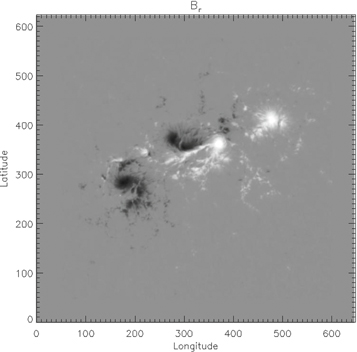
Figure 16. Average Br taken from test data series, from 2011 February 14, 23:35–23:47. The linear gray scale is from −2500 to 2500 G. The image of Br shown here is from the average of the two magnetograms.
Download figure:
Standard image High-resolution image
Figure 17. Average Blon taken from test data series, from 2011 February 14, 23:35–23:47. The linear gray scale is from −2000 to 2000 G. The image of Blon shown here is from the average of the two magnetograms.
Download figure:
Standard image High-resolution image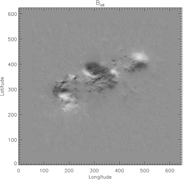
Figure 18. Average Blat taken from test data series, from 2011 February 14, 23:35–23:47. The linear gray scale is from −2000 to 2000 G. The image of Blat shown here is from the average of the two magnetograms.
Download figure:
Standard image High-resolution image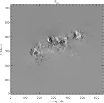
Figure 19. Average Elon taken from test data series, from 2011 February 14, 23:35–23:47. The linear gray scale is from −0.5 to 0.5 V cm−1. The image of Elon shown here is the solution evaluated halfway between the times of the two magnetograms.
Download figure:
Standard image High-resolution image
Figure 20. Average Elat taken from test data series, from 2011 February 14, 23:35–23:47. The linear gray scale is from −0.75 to 0.75 V cm−1. The image of Elat shown here is the solution evaluated halfway between the times of the two magnetograms.
Download figure:
Standard image High-resolution image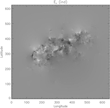
Figure 21. Average  taken from test data series, from 2011 February 14, 23:35–23:47. This figure shows only the inductive contribution to Er. The linear gray scale is from −0.5 to 0.5 V cm−1. The image of
  shown here is the solution evaluated halfway between the times of the two magnetograms.
Download figure:
Standard image High-resolution image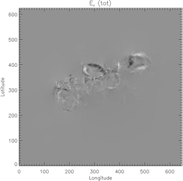
Figure 22. Average Er taken from test data series, from 2011 February 14, 23:35–23:47. This figure shows the total electric field contribution Er. The linear gray scale is from −2 to 2 V cm−1. The image of Er shown here is the solution evaluated halfway between the times of the two magnetograms.
Download figure:
Standard image High-resolution image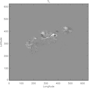
Figure 23. Average radial component of Poynting flux Sr taken from test data series, from 2011 February 14, 23:35–23:47. The linear grayscale range is from −8 to 8 ×10⁹ erg cm−2 s−1. The image of Sr shown here is the solution evaluated halfway between the times of the two magnetograms.
Download figure:
Standard image High-resolution imageBecause the ANMHD simulation was performed in Cartesian coordinates, the first task is to use the formalism described in Section 7 to map the Cartesian domain onto a small surface patch bisected by the equator on a very large sphere. The resulting radius of the sphere in this case is 9.998 × 10⁸ km, well over 1000 times larger than R⊙. The colatitude range b–a = 10−4 rad, and it is also equal to the longitude range d–c, since the domain is a square in Cartesian coordinates.
There is a subroutine in the PDFI_SS library, pdfi_wrapper4anmhd_ss, which closely mimics the functionality of subroutine pdfi_wrapper4jsoc_ss, but with some differences needed to accommodate this special case (for example, no "zero padding" is done by the latter subroutine, since padding was also not done in Kazachenko et al. 2014). test_anmhd.f calls this subroutine and then writes the results to an output file. When the resulting electric field solutions are compared with those from the ANMHD simulation itself, our use of the staggered grid means that the comparison is a little more complicated than it was in Kazachenko et al. (2014). First, so that we can compare quantities directly, we must interpolate the simulation magnetic and electric fields from a centered grid (which the simulation used) to our staggered grid locations; this step was not necessary for the comparison in Section 4 of Kazachenko et al. (2014). Second, because the magnetic field time derivatives were not masked in Kazachenko et al. (2014), we also do not mask them here (in contrast to what is done with HMI data in pdfi_wrapper4jsoc_ss). Similarly, we also did not mask the FLCT electric field or the ideal electric field. However, we found that if we did not mask the Doppler contribution to the electric field, noise in the definition of the  unit vector in the weak-field regions would wreak havoc on the solutions; therefore, we did use the strong-field mask on the Doppler electric field solutions. The threshold for the strong magnetic field mask is 370 G, chosen to be consistent with the threshold used in Kazachenko et al. (2014).
The output file anmhd_output_file_pdfi_ss.sdf from test_anmhd.f can be read into an IDL session with sdf_read_varlist. There is an extensive amount of diagnostic data that can be analyzed, as detailed in the documentation near the front of the file test_anmhd.f. Here, we display just a few aspects of this output data, where the results can be compared with those of Kazachenko et al. (2014). Figures 24–26 show side-by-side comparisons of the longitudinal, latitudinal, and radial electric field images, with the ANMHD simulation results on the left side of the figures, while the PDFI_SS inversion results are shown on the right side of the figures. Both the ANMHD simulation results and the PDFI_SS results have been multiplied by the strong magnetic field masks, as was done for similar figures in Kazachenko et al. (2014). Figure 27 shows the side-by-side comparison of the radial Poynting flux. Finally, Figure 28 shows a scatterplot of the radial component of the Poynting flux from the inversion versus that from the ANMHD simulation and provides a good indication of the resulting error levels from the inversion.
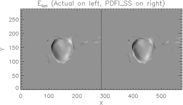
Figure 24. Longitudinal component of the electric field from the ANMHD simulation (left side) and from the PDFI_SS inversion (right side). The linear grayscale range is from −1 to 1 V cm−1. Both contributions have been multiplied by the strong-field mask for the TE grid.
Download figure:
Standard image High-resolution image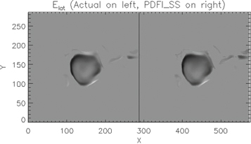
Figure 25. Latitudinal component of the electric field from the ANMHD simulation (left side) and from the PDFI_SS inversion (right side). The linear grayscale range is from −1 to 1 V cm−1. Both contributions have been multiplied by the strong-field mask for the PE grid.
Download figure:
Standard image High-resolution image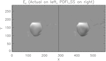
Figure 26. Radial component of the electric field from the ANMHD simulation (left side) and from the PDFI_SS inversion (right side). The linear grayscale range is from −3 to 3 V cm−1. Both contributions have been multiplied by the strong-field mask for the COE grid.
Download figure:
Standard image High-resolution image
Figure 27. Radial component of the Poynting flux from the ANMHD simulation (left side) and from the PDFI_SS inversion (right side). The linear grayscale range is from −5 to 5 ×10¹⁰ erg cm−2 s−1. Both contributions have been multiplied by the strong-field mask for the CE grid.
Download figure:
Standard image High-resolution image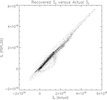
Figure 28. Scatterplot of the radial component of the Poynting flux from the PDFI inversion (y-axis) vs. that from the ANMHD simulation (x-axis). Both contributions have been multiplied by the strong-field mask for the CE grid.
Download figure:
Standard image High-resolution imageOverall, while we find that the ANMHD electric field results are recovered well, we find that the quality of the inversion is not as good as it was for the centered grid case used in Kazachenko et al. (2014). There are a number of possible reasons for this, including the fact that the simulation data must be interpolated to the staggered grid locations and the fact that in the PDFI_SS inversions Faraday's law is obeyed to roundoff error, whereas in the simulation data it is not, as one can see in the bottom right panel of Figure 1 of Welsch et al. (2007). The latter is a consequence of the ANMHD simulations being run with spectral techniques used to compute spatial derivatives, whereas the curl of the simulation data was computed using finite differences. In spite of these differences, these figures show clearly that the PDFI_SS technique is able to reproduce the main morphological features and amplitudes of the ANMHD electric fields.
9.3. test_bpot.f (Executable xbpot)
The potential field software described in Section 6 is tested by test_bpot.f, in which the radial magnetic field on the CE grid at the photosphere is used to compute a potential magnetic field distribution in the volume above the photosphere. In the test program, the angular resolution of the solution is the same as that for the photospheric data. In radius, the test program assumes 1000 voxels in the radial direction, with a source surface height of 2 R⊙ (i.e., one solar radius above the photosphere). The user can choose whether to assume periodic boundary conditions in ϕ by setting the variable bcn to 0 or homogeneous Neumann boundary conditions in ϕ on the poloidal potential P by setting bcn to 3. The test program takes at least several minutes to run (about 10 minutes on a MacBook Pro with 16 GB of memory and a solid-state disk). With limited amounts of memory, it will likely take considerably longer.
The executable xbpot produces an output file, test_bpot_output.sdf, with a series of 2D and 3D arrays. The file can be read in using IDL procedure sdf_read_varlist. Reading in the file can take a long time, as the output file is very large. Once the file is read in, one can type the "help" command in IDL to see the list of output arrays. The solution for the poloidal potential P is stored in the 3D array scrb3d. The three magnetic field components for the solution are computed two different ways: First, subroutines brpot_ss and bhpot_ss are called to compute Br and  using the poloidal potential P as input. The resulting 3D magnetic field arrays are brpot3d, btpot3d, and bppot3d. Second, subroutine ahpot_ss is used to compute the vector potential
  from P. The theta and phi components of the vector potential are returned into the 3D arrays atpot and appot. Then, the three magnetic field components can be computed from the vector potential with subroutine curlahpot_ss. The resulting three 3D magnetic field arrays are brpotvp, btpotvp, and bppotvp. We find that the magnetic field components computed in the two different ways differ very little.
It is important to note that the potential field solution is computed on the faces of the voxels, as described in Section 6, and that the horizontal magnetic field components at the bottom layer in the 3D arrays are located half a voxel above the photosphere. The photospheric values of the potential field components are computed with subroutine bhpot_phot_ss and output into the 2D arrays btpotphot and bppotphot.
Note that all of these output arrays are stored in colatitude–longitude-radius index order. The following test program will take the output file from this test program and rotate some of the 3D arrays into longitude–latitude-radius index order.
9.4. test_bptrans.f (Executable xbptrans)
The test program test_bptrans.f uses the 3D transpose subroutines ahpottp2ll_ss, bhpottp2ll_ss, and brpottp2ll_ss to transpose the 3D arrays computed by test_bpot.f from colatitude–longitude index order to longitude–latitude index order. The program uses the output file from test_bpot.f as an input file and writes transposed output arrays into the file test-inplace-transpose.sdf. The contents of the file can be read into an IDL session using sdf_read_varlist. The arrays in the file include the 3D arrays alon and alat, the longitudinal and latitudinal components of the vector potential, respectively, and blonpot, blatpot, and brllpot, the 3D arrays of the longitudinal, latitudinal, and radial components of  , respectively. The transposed 2D photospheric magnetic field components are in the arrays blonphot and blatphot.
When working with large 3D arrays such as these, we used a memory-saving technique in FORTRAN that is worth describing. Instead of having to create two separate arrays of the same size, but with different shapes, it is possible, using a combination of C and FORTRAN pointers, to create the two separate arrays such that they occupy the same locations in memory but still have different shapes. The two different array names can then be successfully passed as arguments into our PDFI_SS 3D transpose subroutines. We will now illustrate how we do this using the radial magnetic field component of the potential field solution as an example.
The ability to combine the usage of C and FORTRAN pointers can be invoked by the declaration use, intrinsic :: iso_c_binding
within a FORTRAN program. The original array brpot in colatitude–longitude index order is declared as a third-rank allocatable array: real*8, allocatable,target :: brpot(:,:,:). The transposed array, brllpot, is declared as a third-rank FORTRAN pointer: real*8, pointer :: brllpot(:,:,:).
We also define the two shape arrays integer :: shapebrpot(3), shll(3).
Then, one defines and reads in the integers m,n,p. The array brpot is then allocated as allocate brpot(m,n,p+1).
Once the array is allocated, its shape can be determined with the FORTRAN shape function: shapebrpot=shape(brpot).
The shape of the transpose array can then be determined by the following three statements: shll(1)=shapebrpot(2) shll(2)=shapebrpot(1) shll(3)=shapebrpot(3).
The next step is to read in the brpot array from the input file. Once that is done, we can assign the FORTRAN pointer for the transposed array: call c_f_pointer(c_loc(brpot),brllpot,shll).
What this statement does is define the brllpot array to occupy the same location in memory as the brpot array, but with the shape of the transpose array. One can then call the PDFI_SS subroutine brpottp2ll_ss, with the brpot array as input and brllpot as the output array: call brpottp2ll_ss(m,n,p,brpot,brllpot).
The source code for brpottp2ll_ss is written in such a way that the transpose is done sequentially for each horizontal layer of the 3D arrays, with a copy of the 2D array made before any transpose operation has been done. Thus, the 3D transpose can be done "in place," without destroying any data. It is very important to note that once the 3D transpose subroutine has been called, the original untransposed array is essentially destroyed by scrambling it into the new shape and is hence useless. Thus, the 3D transpose operation should be the last operation done using the original array.
This concept is used for all the 3D transpose operations in test_bptrans.f. The contents of the output file were used to generate the potential field figures shown in Section 6.2.
9.5. test_psipot.f (Executable xpsipot)
The purpose of the test_psipot.f test program is to test the ability to compute the potential magnetic field by using the observed horizontal components of the magnetic field at the photosphere as input. These solutions are computed by subroutines psipot_ss and bpot_psi_ss, as described in Section 6.7. On input, the test program reads in arrays of the observed horizontal magnetic fields at the photosphere at the staggered grid locations from file test-fortran-input.sdf, and on output it computes the scalar potential Ψ and the 3D magnetic field components, all in colatitude–longitude-radius index order. The results of the potential field calculation are written to the output file test-psipot-output.sdf.
The solution for the scalar potential Ψ is returned as two separate 3D arrays, psi3d, which assumes zero net radial flux, and psi3df, in which a net radial flux is imposed with subroutine psi_fix_ss that coincides with the net radial flux from the observed radial components of the magnetic field. The potential magnetic field components are computed with bpot_psi_ss and are given in the arrays btpot3d, bppot3d, and brpot3d. Photospheric values of the horizontal potential magnetic field components are given in the 2D arrays btpot and bppot. The horizontal divergences of the observed photospheric horizontal magnetic fields are given in the 2D array divbh, and the divergences of the potential photospheric horizontal magnetic fields are given in the 2D array divbhpot.
As an alternative to the observed horizontal magnetic field components in test-fortran-input.sdf, one can instead change the input file name to test-fortran-inputpotphot.sdf, where in this case the horizontal components of  are computed from the potential magnetic field solution chosen to match Br. In this case, the radial magnetic field component computed by test_psipot.f should be close to the observed radial magnetic field component. The error between the two was shown earlier in Figure 14.
One can choose to use periodic boundary conditions in ϕ by setting the variable bcn to 0 in test_psipot.f, or homogeneous Neumann boundary conditions by setting bcn to 3. For this test case, homogeneous Neumann boundary conditions require more compute time.
9.6. test_global.f (Executable xglobal)
The test program test_global.f is designed to test the ability of subroutine enudge3d_gl_ll to compute a global (4π sr) PTD solution covering the entire surface of the Sun. On input, arrays of  ,
,  , and
, and  defined on the PE, TE, and CE grids, respectively, spanning the global Sun, are computed from two sets of vector magnetogram data, using a temporal finite difference to define the time derivative. In this case, we have used AR 11158 vector magnetogram data and mapped them onto the global Sun geometry, setting a = 0, b = π, c = 0, and d = 2π, i.e., we have allowed AR 11158 to take over the entire surface of the Sun. Because in a global geometry we cannot have a nonzero net radial magnetic flux, or its time derivative, we use subroutine fluxbal_ll to zero out the average before calling enudge3d_gl_ll, which computes
  on all the rails of the spherical voxels, which are bisected in radius by the photosphere.
To test whether this global solution for  obeys all three components of Faraday's law, we compute the curl of
  with subroutine curle3d_ll, which can accommodate both spherical wedge and global geometries. The resulting components of the curl of
  can then be compared against the input time derivatives
  ,
,  , and
, and  . The documentation near the top of test_global.f provides the names of the appropriate arrays for the time derivatives and the three components of the curl of
  , as well as the arrays for
  itself. Scatter plots of the curl of
  versus the magnetic field time derivatives should show straight lines for each component. The output file for test_global.f is global_test_out_ar11158.sdf, and the contents of the file can be read in with IDL procedure sdf_read_varlist.
9.7. test_interp.f (Executable xinterp)
In Section 3.13, we described several subroutines designed to use a B-spline to interpolate the input data for computing PDFI electric field inversions to a different resolution. Here, the test program test_interp.f performs a test of this B-spline interpolation, by first interpolating an observed HMI image of Br, which includes regions of zero padding, to a new resolution that is about 20% higher than the original resolution, and then it reinterpolates that image back to the original resolution. The original Br data array can then be compared directly to the twice-interpolated array of the same size, and the quality of the twice-interpolated image can be evaluated. The output file, brint.sdf, contains the original image as the array brdat, the interpolation to the higher resolution as the array brint, and the twice-interpolated array as brback. The test program uses the subroutine interp_hmidata_ll to perform the interpolations. The default value of the degree of the spline, deg, is set to 9, but the user can experiment with other values. Allowed values are 3, 5, 7, and 9. Thus far we have found that setting deg=9 seems to produce the most accurate results. The output file can be read in with the IDL procedure sdf_read_varlist to study the results.
9.8. test_pdfi_c.c (Executable xctest)
In Section 8.5, we described the principles of calling PDFI_SS subroutines from C/C++ programs. In the test program test_pdfi_c.c, we illustrate many of the important points made in that section with this very simple test program, which calls a single PDFI_SS subroutine, brll2tp_ss. This test program (1) illustrates how to define a 1D array in C that maps onto 2D arrays in FORTRAN, (2) shows how to define the input array in column-major order, consistent with its use in FORTRAN, (3) shows that calling arguments are all called by reference, and (4) uses the output array to demonstrate the column-major nature of the output generated by the FORTRAN subroutine.
In the C test program, pointers for the arrays brll (the input array) and br (the output array) are defined and initialized to NULL. Next, integer variables np1 and mp1 (representing n + 1 and m + 1, respectively) are defined and set to 12 and 10, respectively. The integers m and n are then defined by decrementing np1 and mp1 by one. Next, the input and output arrays brll and br are each allocated to have the size (n + 1) ∗ (m + 1), i.e., the product of the FORTRAN dimensions. Next, the array brll is defined so that regarded as a FORTRAN array, the value of brll(j,i)=(i-1)+(j-1). This is done by using an outer loop over the latitude index i that goes from 0 to m and an inner loop over the longitude index j that goes from 0 to n. The calculation of the array value is brll[i∗np1+j]=(double) i + j;. This is the essence of constructing the array in C to have column-major order, before the FORTRAN subroutine is called. Note that the j index is the most rapidly varying. (The values of i and j differ between C and FORTRAN because in FORTRAN the default index values start from 1 whereas in C they start from 0.)
Next, the FORTRAN subroutine brll2tp_ss is called: brll2tp_ss_ (&m, &n, brll, br);. Note the trailing underscore in the subroutine name and the fact that the pointers to m and n are used in the call (the arrays brll and br are already defined as pointers).
Following the subroutine call, both the brll and br arrays are printed to the screen. In the loop that prints the values of brll, the outer loop is over the latitude index and the inner loop is over the longitude index, consistent with column-major order in FORTRAN. When printing out the output array br to the screen, column-major ordering results in the colatitude index i varying most rapidly, and the longitude index j varies more slowly: the outer loop is over j, and the inner loop is over i. The FORTRAN array br(i,j) is indexed in C as br[j∗mp1+i].
These same principles in setting up 1D arrays in C that map onto multidimensional FORTRAN arrays should work for any of the subroutines in PDFI_SS, as long as one pays careful attention to the dimensions of the arrays defined in the FORTRAN subroutines and remembers that FORTRAN assumes that the arrays are defined in column-major index order.
When running the executable xctest, the array brll is printed to the screen, followed by its colatitude–longitude transpose, br.
9.9. Python Linking Test Program
We have prepared an example of the PDFI_SS-Python linking described in Section 8.6 in the subfolder fortran/test-programs/python-linking. The package contains a working signature file pdfi_ss.pyf created for routines add_padding_as_ss, pad_abcd_as_ss, pad_int_gen_ss, and pdfi_wrapper4jsoc_ss in the PDFI_SS library. The F2PY extension module pdfi_ss.so can be compiled by typing "make" in the terminal while within the subfolder python-linking. Typing "make clean" removes the extension module. The fishpack library location must be correctly specified in the Makefile, and the FISHPACK library must be compiled with the -fPIC flag (see discussion in Section 8.3).
The Python script pdfi_wrapper4jsoc_script.py imports the Python interfaces of the PDFI_SS subroutines from the compiled extension module and calls them to process the input data and to estimate the electric field by calling the pdfi_wrapper4jsoc_ss subroutine (Section 3.11). Thus, the script reproduces the first part of the test program test_wrapper.f (Section 9.1). The input data required by the pdfi_wrapper4jsoc_ss can be downloaded in Python-compatible .sav format from the URL described in the introduction to Section 9. In pdfi_wrapper4jsoc_script.py, the output arrays of pdfi_wrapper4jsoc_ss are returned as NumPy arrays, and the script saves them to a NumPy .npz file. This output can be then compared to the output of the pure FORTRAN version of pdfi_wrapper4jsoc_ss executed within test_wrapper.f. Example output files created by executing test_wrapper.f can be downloaded from the above URL in Python-compatible .sav format, and their content can be compared to the output of the pdfi_wrapper4jsoc_script.py using the compare_wrapper_outputs.py script. The differences printed by the script should be small and close to floating-point precision.
If the user wishes to do the comparison from scratch on his/her local system, the package includes also IDL helper scripts for transforming the .sdf input and output files of test_wrapper.f program into Python-compatible .sav format. The README.txt file in this subfolder contains also step-by-step instructions for creating the F2PY interface from scratch.
10. List of Subroutines and Common Arguments Used in PDFI_SS
This article discusses the most important FORTRAN subroutines within PDFI_SS. We first make a brief note on some conventions used in the software regarding suffixes of the subroutine names. Most of the subroutine names in PDFI_SS end with the suffix _ss, to denote the "spherical-staggered" grid assumptions, but there are some important exceptions. For those subroutine names that end in _ll, it is assumed that the input and output array arguments are arranged in "longitude–latitude" index order, in contrast to the "colatitude–longitude" array index order used by most of the subroutines. See Section 3.2 for a general discussion of the distinction between these two array indexing schemes. A few subroutines end with the suffix _sc, denoting "spherical centered," meaning that for these cases a centered rather than a staggered grid description is assumed.
We provide a list in alphabetical order of the most important subroutines in the PDFI_SS library (in Table 3), as well as a list of commonly used arguments in the subroutines, along with brief descriptions. The list of subroutines also includes a brief statement of purpose and links to the section in the article where more detailed discussion of the subroutine occurs.
Table 3. Subroutine Name, Purpose, and Section
| Subroutine Name | Purpose | Section |
|---|---|---|
| abcd2wcs_ss | Compute WCS/FITS keywords from a,b,c,d | Section 3.6 |
| add_padding_as_ss | Insert unpadded data array into padded data array | Section 4.5 |
| ahpot_ss | Compute vector potential in 3D for potential magnetic field from poloidal potential P | Section 6.2 |
| ahpottp2ll_ss | Transpose 3D vector potential for potential field from colat–lon to lon–lat index order | Section 6.6 |
| angle_be_ss | Compute angle between  and and 
|
Section 3.9.2 |
| berciktest_ss | Test accuracy of solution for P to Bercik's equation | Section 6.1.7 |
| bhll2tp_ss | Transpose COE arrays of  from lon–lat to colat–lon order from lon–lat to colat–lon order |
Section 3.6 |
| bhpot_phot_ss | Compute horizontal potential magnetic field at photosphere | Section 6.2 |
| bhpot_ss | Compute  for potential magnetic field in 3D volume from poloidal potential P for potential magnetic field in 3D volume from poloidal potential P |
Section 6.2 |
| bhpottp2ll_ss | Transpose 3D arrays of potential field  from colat–lon to lon–lat order from colat–lon to lon–lat order |
Section 6.6 |
| bhtp2ll_ss | Transpose COE arrays of  from colat–lon to lon–lat order from colat–lon to lon–lat order |
Section 3.6 |
| bhyeell2tp_ss | Transpose staggered grid arrays of  from lon–lat to colat–lon order from lon–lat to colat–lon order |
Section 3.6 |
| bhyeetp2ll_ss | Transpose staggered grid arrays of  from colat–lon to lon–lat order from colat–lon to lon–lat order |
Section 3.6 |
| bpot_psi_ss | Compute potential magnetic field from Ψ in 3D | Section 6.7.2 |
| br_voxels3d_ss | Compute Br on top and bottom faces of voxels from  , Br at radial midpoint , Br at radial midpoint |
Section 6.7.2 |
| brll2tp_ss | Transpose Br on COE grid from lon–lat to colat–lon order | Section 3.6 |
| brpot_ss | Compute Br for potential magnetic field in 3D volume from poloidal potential P | Section 6.2 |
| brpottp2ll_ss | Transpose 3D potential field array Br from colat–lon to lon–lat order | Section 6.6 |
| brtp2ll_ss | Transpose Br on COE grid from colat–lon to lon–lat order | Section 3.6 |
| bryeell2tp_ss | Transpose Br on staggered grid from lon–lat to colat–lon order | Section 3.6 |
| bryeetp2ll_ss | Transpose Br on staggered grid from colat–lon to lon–lat order | Section 3.6 |
| bspline_ss | Low-level routine for B-spline interpolation | Section 3.13 |
| car2sph_ss | Compute radius of sphere to use for Cartesian solutions | Section 7 |
| curl_psi_rhat_ce_ss | Compute  for ψ on CEG grid for ψ on CEG grid |
Section 3.7 |
| curl_psi_rhat_co_ss | Compute  for ψ on COE grid for ψ on COE grid |
Section 3.7 |
| curlahpot_ss | Compute  × ×  for potential magnetic field in 3D volume for potential magnetic field in 3D volume |
Section 6.2 |
| curle3d_ll | Compute  × ×  for for  voxel arrays in lon–lat order voxel arrays in lon–lat order |
Section 5.4 |
| curle3d_ss | Compute  × ×  for for  voxel arrays in colat–lon order voxel arrays in colat–lon order |
Section 5.4 |
| curle3dphot_ss | Compute  × ×  for for  evaluated at photosphere evaluated at photosphere |
Section 5.4 |
| curlehr_ss | Compute  for for  arrays in colat–lon order arrays in colat–lon order |
Section 5.4 |
| curlh_ce_ss | Compute  evaluated on CE grid evaluated on CE grid |
Section 3.7 |
| curlh_co_ss | Compute  evaluated on CO grid evaluated on CO grid |
Section 3.7 |
| dehdr_ss | Compute radial derivatives of horizontal electric fields evaluated at photosphere | Section 5.4 |
| delh2_ce_ss | Compute horizontal Laplacian of ψ at CE grid locations for ψ on CEG grid | Section 3.7 |
| delh2_co_ss | Compute horizontal Laplacian of ψ at CO grid locations for ψ on COE grid | Section 3.7 |
| divh_ce_ss | Compute divergence of horizontal components of a vector at CE grid locations | Section 3.7 |
| divh_co_ss | Compute divergence of horizontal components of a vector at CO grid locations | Section 3.7 |
| divh_sc | Compute divergence of horizontal components of a vector using centered grid formalism | Section 3.9.2 |
| downsample3d_ll | Flux-preserving downsampling of three-component electric field in lon–lat order | Section 5.1 |
| downsample3d_ss | Flux-preserving downsampling of three-component electric field in colat–lon order | Section 5.1 |
| downsample_ll | Flux-preserving sownsampling of two-component electric field in lon–lat order | Section 5.1 |
| downsample_ss | Flux-preserving downsampling of two-component electric field in colat–lon order | Section 5.1 |
| e_doppler_rpils_ss | Experimental technique to compute Doppler electric field using radial and LOS PILs | Section 3.9.3 |
| e_doppler_ss | Default technique to compute noninductive Doppler electric field | Section 3.9.3 |
| e_flct_ss | Compute noninductive electric field from FLCT velocities | Section 3.9.4 |
| e_ideal_ss | Compute noninductive ideal electric field, minimizing 
|
Section 3.9.5 |
| e_laplace_ll | Compute curl-free electric field using Et assuming lat–lon order | Section 5.1 |
| e_laplace_ss | Compute curl-free electric field using Et assuming colat–lon order | Section 5.1 |
| e_ptd_ss | Compute inductive (PTD) electric field components given  and and 
|
Section 3.9.1 |
| ehyeell2tp_ss | Transpose horizontal electric field on staggered grid from lon–lat to colat–lon order | Section 3.6 |
| ehyeetp2ll_ss | Transpose horizontal electric field on staggered grid from colat–lon to lon–lat order | Section 3.6 |
| emagpot_psi_ss | Compute potential field magnetic energy from Br and ψ at photosphere | Section 6.5 |
| emagpot_srf_ss | Compute potential field magnetic energy from  and and  at photosphere at photosphere |
Section 6.5 |
| emagpot_ss | Compute potential field magnetic energy by integrating B2/(8π) over volume | Section 6.5 |
| enudge3d_gl_ll | Compute three-component global nudging electric field in lon–lat order | Section 5.3 |
| enudge3d_gl_ss | Compute three-component global nudging electric field in colat–lon order | Section 5.3 |
| enudge3d_ss | Compute three-component Nudging electric field in colat–lon order | Section 5.2 |
| enudge_gl_ll | Compute two-component global nudging electric field in lon–lat order | Section 5.3 |
| enudge_gl_ss | Compute two-component global nudging electric field in colat–lon order | Section 5.3 |
| enudge_ll | Compute two-component nudging electric field in lon–lat order | Section 5.2 |
| enudge_ss | Compute two-component nudging electric field in colat–lon order | Section 5.2 |
| eryeell2tp_ss | Transpose radial electric field from lon–lat to colat–lon order | Section 3.6 |
| eryeetp2ll_ss | Transpose radial electric field from colat–lon to lon–lat order | Section 3.6 |
| find_mask_ss | Compute strong-field mask on COE grid | Section 3.6 |
| fix_mask_ss | Convert intermediate interpolated mask values to 0 or 1 | Section 3.6 |
| fluxbal_ll | Remove net radial magnetic flux from Br assuming lon–lat order | Section 5.3 |
| fluxbal_ss | Remove net radial magnetic flux from Br assuming colat–lon order | Section 5.3 |
| gradh_ce_ss | Compute horizontal gradient of ψ for ψ on CEG grid | Section 3.7 |
| gradh_co_ss | Compute horizontal gradient of ψ for ψ on COE grid | Section 3.7 |
| gradh_sc | Compute horizontal gradient of ψ using centered grid formalism | Section 3.9.2 |
| hm_ss | Compute helicity injection rate contribution function | Section 3.10 |
| hmtot_ss | Compute helicity injection rate over photospheric domain | Section 3.10 |
| interp_data_ss | Interpolate several arrays from COE grid to staggered grid locations | Section 3.6 |
| interp_eh_ss | Interpolate horizontal electric fields from staggered grid locations to CO grid | Section 3.9.2 |
| interp_hmidata_3d_ll | Interpolate 18 COE input data arrays to a different resolution using B-spline | Section 3.13 |
| interp_hmidata_ll | Interpolate a single COE input data array to a different resolution using B-spline | Section 3.13 |
| interp_var_ss | Interpolate three components of a vector from COE to staggered grid locations | Section 3.6 |
| kcost_ss | Compute wavenumbers assuming homogenous Neumann boundary conditions in ϕ | Section 6.1.4 |
| kfft_ss | Compute wavenumbers assuming periodic boundary conditions in ϕ | Section 6.1.4 |
| laplacetest_ss | Test the accuracy of the solution for ψ to the 3D Laplace equation | Section 6.7.1 |
| mflux_ss | Compute the net magnetic flux over the photospheric spherical wedge domain | Section 6.2 |
| pad_abcd_as_ss | Compute new values of a, b, c, and d given the old values and the amounts of padding | Section 4.5 |
| pad_int_gen_ss | Compute amounts of padding on all four boundaries | Section 4.5 |
| pdfi_wrapper4anmhd_ss | Compute PDFI solution for  for the ANMHD test case for the ANMHD test case |
Section 9.2 |
| pdfi_wrapper4jsoc_ss | Compute PDFI solution for  for a cadence of vector magnetogram and Doppler data for a cadence of vector magnetogram and Doppler data |
Section 3.11 |
| psi_fix_ss | Remove 1/r artifact from Ψ and impose observed net magnetic flux (if desired) | Section 6.7.1 |
| psipot_phot_ss | Compute Ψ at photosphere from Br and poloidal potential P | Section 6.5 |
| psipot_ss | Compute Ψ for a potential field using  at photosphere, solving the Laplace equation at photosphere, solving the Laplace equation |
Section 6.7.1 |
| ptdsolve_eb0_ss | Compute  , ,  , and , and  by solving Poisson equations assuming Et = 0 by solving Poisson equations assuming Et = 0 |
Section 3.9.1 |
| ptdsolve_ss | Compute  , ,  , and , and  by solving Poisson equations using nonzero Et by solving Poisson equations using nonzero Et |
Section 3.9.1 |
| relax_psi_3d_ss | Solve for scalar potential ψ using the "iterative" method formulated by Brian Welsch | Section 3.9.2 |
| scrbpot_ss | Solve Bercik's equation for the poloidal potential P for a potential magnetic field in 3D | Section 6.1 |
| sinthta_ss | Compute  at colatitude cell edges and cell centers at colatitude cell edges and cell centers |
Section 3.7 |
| sr_ss | Compute radial component of the Poynting flux at the photosphere | Section 3.10 |
| srtot_ss | Integrate the radial Poynting flux over area to derive magnetic energy input rate | Section 3.10 |
| wcs2abcd_ss | Compute a, b, c, and d from WCS/FITS keywords for COE grid | Section 3.6 |
| wcs2mn_ss | Compute m and n from WCS/FITS keywords | Section 3.6 |
Now we list and describe some of the most commonly used calling argument variables used in the subroutines within PDFI_SS, as well as important information about these variables.
10.1. Common Input Variables Defining Domain Geometry
- 1.rsun [km]: This real*8 scalar variable defines the radius of the photospheric surface upon which the PDFI calculations will be done. The expected units are km. For most solar applications, this can be set to 6.96d5. But if you are computing solutions in Cartesian geometries, this variable is typically set to a much larger number (see Section 7).
- 2.a,b,c,d [rad]: These four real*8 scalar variables define the 2D "spherical wedge" subdomain used in PDFI_SS (see Section 3.1). The quantity a defines the colatitude of the northern domain edge, b defines the colatitude of the southern domain edge, and c and d define the longitude values of the left and right domain edges, respectively. The quantity a is less than b, and both are bounded below by 0 and above by π. The quantity c is less than d, and both are nominally in the range from 0 to 2π.
- 3.m,n: These 32 bit integer values set the number of cell interiors in colatitude and longitude, respectively. Nearly all array dimensions in PDFI_SS subroutines are defined in terms of these integers.
- 4.p: This 32 bit integer sets the number of radial voxels used in calculations of potential magnetic field solutions in three dimensions. The array sizes for the 3D arrays in the potential magnetic field software are defined in terms of m, n, and p.
- 5.dtheta, dphi [rad]: These two real*8 scalar variables describe the size of the colatitude and longitude cells in a Plate Carrée grid and are assumed to be constant within the spherical wedge domain. Their values are defined by Equations (31) and (32) in Section 3.1. The PDFI_SS software does not make any assumptions about the relative size of dtheta and dphi, but in the HMI magnetic pipeline software we attempt to keep dtheta and dphi nearly equal.
- 6.dr [km]: This real*8 scalar variable describes the radial depth of spherical voxels used in subroutines e_voxels3d_ss, br_voxels3d_ss, enudge3d_ss, enudge3d_gl_ss, enudge3d_gl_ll, curle3d_ss, and curle3d_ll. In these subroutines, the bottom faces and edges of the voxels lie 0.5∗dr below the photosphere, and the top faces and edges of the voxels lie 0.5∗dr above the photosphere.
- 7.sinth(m+1), sinth_hlf(m): These two real*8 arrays contain values of (where θ is colatitude), evaluated at colatitude cell edges (sinth) and colatitude cell centers (sinth_hlf). These two arrays can be computed with subroutine sinthta_ss.
- 8.rssmrs [km]: This real*8 scalar variable is used by the potential magnetic field software and denotes the distance between the radius of the Sun (rsun) and the source surface outer boundary.

10.2. Input Magnetic Field and Velocity Variables Passed into pdfi_wrapper4jsoc_ss
All the input magnetic field, LOS unit vector, and velocity variables that are passed into subroutine pdfi_wrapper4jsoc_ss are defined on the COE grid and are given in longitude–latitude index order. All 18 of these real*8 arrays are dimensioned (n + 1, m + 1). Variable names ending in 0 refer to the first of the two time steps, and names ending in 1 refer to the second of the two time steps. See discussion in Section 3.6. We also include in this list the scalar bmin, which sets the threshold for the strong-field mask.
- 1.bmin [G]: real*8 scalar that determines the threshold for the strong-field mask array on the COE grid. The quantity must be larger than bmin at both input time steps for the mask value to be set to 1.
- 2.bloncoe0, bloncoe1 [G]: arrays of the longitudinal component of the magnetic field at the first and second time steps, respectively.
- 3.blatcoe0, blatcoe1 [G]: arrays of the latitudinal component of the magnetic field at the first and second time steps, respectively.
- 4.brllcoe0, brllcoe1 [G]: arrays of radial component of the magnetic field at the first and second time steps, respectively.
- 5.lloncoe0, lloncoe1: arrays of longitudinal component of the unit vector pointing toward the observer at the first and second time steps, respectively.
- 6.llatcoe0, llatcoe1: arrays of latitudinal component of the unit vector pointing toward the observer at the first and second time steps, respectively.
- 7.lrllcoe0, lrllcoe1: arrays of the radial component of the unit vector pointing toward the observer at the first and second time steps, respectively.
- 8.vloncoe0, vloncoe1 [km s−1]: arrays of the longitudinal component of the optical flow velocity computed by FLCT at the first and second time steps, respectively (see discussion in Section 4.4).
- 9.vlatcoe0, vlatcoe1 [km s−1]: arrays of the latitudinal component of the optical flow velocity computed by FLCT at the first and second time steps, respectively (see discussion in Section 4.4).
- 10.vlosllcoe0, vlosllcoe1 [m s−1]: arrays of the LOS component of the velocity, with positive values denoting redshifts, at the first and second time steps, respectively. Note units difference c.f. FLCT velocities.

10.3. Output Magnetic Field and Electric Field Variables from pdfi_wrapper4jsoc_ss
On output from pdfi_wrapper4jsoc_ss, magnetic field variables at both time steps are returned on their staggered grid locations, as well as the electric field solution variables, computed midway between the two time steps, also on their staggered grid locations. The radial Poynting flux array is returned, as well as its spatial integral. The helicity injection rate contribution function is also returned, along with its spatial integral, the relative helicity injection rate. Strong-field masks for the COE, CO, CE, TE, and PE grids are also returned. All output arrays are in longitude–latitude index order.
- 1.blon0(n+1,m), blon1(n+1,m) [G]: These real*8 arrays of the longitudinal magnetic field component are defined on the PE grid, for the first and second time steps.
- 2.blat0(n,m+1), blat1(n,m+1) [G]: These real*8 arrays of the latitudinal magnetic field component are defined on the TE grid, for the first and second time steps.
- 3.brll0(n,m), brll1(n,m) [G]: These real*8 arrays of the radial magnetic field component are defined on the CE grid, for the first and second time steps.
- 4.elonpdfi(n,m+1) [V cm−1]: This real*8 array of the longitudinal component of the PDFI electric field is defined on the TE grid, evaluated midway between the two time steps. To convert to units of G km s−1, multiply by 1000.
- 5.elatpdfi(n+1,m) [V cm−1]: This real*8 array of the latitudinal component of the PDFI electric field is defined on the PE grid, evaluated midway between the two time steps. To convert to units of G km s−1, multiply by 1000.
- 6.delondr(n,m+1) [V cm−2]: This real*8 array of the radial derivative of the longitudinal component of the PTD electric field is defined on the TE grid, evaluated midway between the two time steps. To convert to units of G s−1, multiply by 108.
- 7.delatdr(n+1,m) [V cm−2]: This real*8 array of the radial derivative of the latitudinal component of the PTD electric field is defined on the PE grid, evaluated midway between the two time steps. To convert to units of G s−1, multiply by 108.
- 8.erllpdfi(n+1,m+1) [V cm−1]: This real*8 array of the radial component of the PDFI electric field is defined on the COE grid, evaluated midway between the two time steps. To convert to units of G km s−1, multiply by 1000. Do not use this array when evaluating the horizontal components of × .
- 9.erllind(n+1,m+1) [V cm−1]: This real*8 array of the inductive (PTD) contribution to the radial electric field is defined on the COE grid, evaluated midway between the two time steps. To convert to units of G km s−1, multiply by 1000. This is the array to use when evaluating the horizontal components of × .
- 10.srll(n,m) [erg cm−2 s−1]: This real*8 array of the radial component of the Poynting flux is defined on the CE grid, evaluated midway between the two time steps.
- 11.srtot [erg s−1]: This real*8 scalar is the area integral of the radial component of the Poynting flux, evaluated midway between the two time steps.
- 12.hmll(n,m) [Mx2 cm−2 s−1]: This real*8 array of the contribution function for the Helicity injection rate is defined on the CE grid, evaluated midway between the two time steps.
- 13.hmtot [Mx2 s−1]: This real*8 scalar is the area integral of the contribution function for the helicity injection rate, evaluated midway between the two time steps.
- 14.mcoell(n+1,m+1): This real*8 array is the strong-field mask for the COE grid, evaluated midway between the two time steps.
- 15.mcoll(n-1,m-1): This real*8 array is the strong-field mask for the CO grid, evaluated midway between the two time steps.
- 16.mcell(n,m): This real*8 array is the strong-field mask for the CE grid, evaluated midway between the two time steps.
- 17.mtell(n,m+1): This real*8 array is the strong-field mask for the TE grid, evaluated midway between the two time steps.
- 18.mpell(n+1,m): This real*8 array is the strong-field mask for the PE grid, evaluated midway between the two time steps.


10.4. The Poloidal and Toroidal Potentials for Electric Field Solutions
The subroutine ptdsolve_ss returns the poloidal and toroidal potentials (or their time derivatives), as well as the radial derivative of the poloidal potential (or its time derivative), at the photospheric surface within our staggered spherical wedge domain. Here we summarize the output variables returned from ptdsolve_ss. Note that when solving the Poisson equations for the PTD potentials, all input and output variables are arranged in colatitude–longitude index order:
- 1.scrb(m+2,n+2) [G km2 or G km2 s−1]: This real*8 array contains the poloidal potential P (or) evaluated on the CEG grid. The name scrb originates from our original notation in KFW14, in which we called the poloidal potential (or "script B"). While we now use the notation P, the array name in the software refers to its original variable name.
- 2.dscrbdr(m+2,n+2) [G km or G km s−1]: This real*8 array contains the radial derivative of the poloidal potential ∂P/∂r (or) evaluated on the CEG grid.
- 3.scrj(m+1,n+1) [G km or G km s−1]: This real*8 array contains the toroidal potential T (or) evaluated on the COE grid. The name scrj originates from our original notation in KFW14, in which we called the toroidal potential (or "script J"). While we now use the notation T, the array name in the software refers to its original variable name.


10.5. Staggered Grid Variable Names of Magnetic and Electric Field Components Commonly Used in PDFI_SS Calculations
As described in Section 3, most of the calculations involving magnetic field and electric field components are performed in colatitude–longitude index order, using the staggered grid locations described in Section 3.4. When magnetic field components are needed (rather than their time derivatives), we use values averaged between the two input time steps, effectively evaluated midway between the two time steps. The electric fields are also evaluated midway between the two time steps. Here we describe magnetic field variable names used in vector calculus subroutines divh_ce_ssand curlh_co_ss and the electric field variable names used on output by e_ptd_ss, as well as on input to the vector calculus subroutines divh_co_ss and curlh_ce_ss. These magnetic and electric field variable names are also frequently used as input or output arguments to many of the transpose subroutines discussed in Section 3.6. In the subroutines e_flct_ss, e_doppler_ss, and e_ideal_ss, variations of these electric field variable names are used on output from these subroutines. Note that when used in the calculation of electric fields, electric field components are computed in units of  , i.e., G km s−1, rather than in the V cm−1 units passed on output from pdfi_wrapper4jsoc_ss.
- 1.bt(m+1,n) [G]: This real*8 array is the colatitude component (Bθ) of the magnetic field, computed on the TE grid, evaluated midway between the two time steps.
- 2.bp(m,n+1) [G]: This real*8 array is the longitude component (Bϕ) of the magnetic field, computed on the PE grid, evaluated midway between the two time steps.
- 3.br(m,n) [G]: This real*8 array is the radial component of the magnetic field, computed on the CE grid, evaluated midway between the two time steps.
- 4.et(m,n+1) [G km s−1]: This real*8 array is the colatitude component of (cEθ), computed on the PE grid, evaluated midway between the two time steps.
- 5.ep(m+1,n) [G km s−1]: This real*8 array is the longitudinal component of (cEϕ), computed on the TE grid, evaluated midway between the two time steps.
- 6.er(m+1,n+1) [G km s−1]: This real*8 array is the radial component of (cEr), computed on the COE grid, evaluated midway between the two time steps.


10.6. Variables Returned from Potential Magnetic Field Subroutines
The subroutine scrbpot_ss returns the 3D array representing the poloidal potential P, subroutine ahpot_ss returns the two 3D arrays representing the vector potential  , subroutine bhpot_ss returns the two 3D arrays representing the horizontal components of
  , and subroutine brpot_ss returns the 3D array of the radial component of
  . If desired, all three components of
  can be computed from the vector potential
  using subroutine curlahpot_ss. Here is a list of these returned variables:
- 1.scrb3d(m,n,p+1) [G km2]: This 3D real*8 array is the poloidal potential P for the potential magnetic field solution returned from subroutine scrbpot_ss. This array can be used to generate the vector potential and magnetic field components for the potential magnetic field solution. This variable is evaluated on the CE grid (horizontal directions), on radial shells.
- 2.mflux [G km2]: This real*8 scalar is the net signed photospheric radial magnetic flux, returned from subroutine mflux_ss. This variable is used on input to subroutines ahpot_ss and brpot_ss to compute potential magnetic field solutions with nonzero net radial photospheric magnetic flux. To compute solutions with zero net radial magnetic flux, one can set mflux to zero.
- 3.atpot(m,n+1,p+1) [G km]: This 3D real*8 array represents, the colatitude component of the vector potential for the potential magnetic field solution, computed by subroutine ahpot_ss. This variable is evaluated on the PE grid (horizontal directions), on radial shells.
- 4.appot(m+1,n,p+1) [G km]: This 3D real*8 array represents, the longitudinal component of the vector potential for the potential magnetic field solution, computed by subroutine ahpot_ss. This variable is evaluated on the TE grid (horizontal directions), on radial shells.
- 5.btpot(m+1,n,p) [G]: This 3D real*8 array represents, the colatitude component of the potential magnetic field solution, computed by subroutine bhpot_ss or curlahpot_ss. This variable is evaluated on the TE grid (horizontal directions), midway between radial shells.
- 6.bppot(m,n+1,p) [G]: This 3D real*8 array represents, the longitudinal component of the potential magnetic field solution, computed by subroutine bhpot_ss or curlahpot_ss. This variable is evaluated on the PE grid (horizontal directions), midway between radial shells.
- 7.brpot(m,n,p+1) [G]: This 3D real*8 array represents, the radial component of the potential magnetic field solution, computed by subroutine brpot_ss or curlahpot_ss. This variable is evaluated on the CE grid (horizontal directions), on radial shells.


This work was supported by NASA and NSF through their funding of the "CGEM" project through NSF award AGS1321474 to UC Berkeley, NASA award 80NSSC18K0024 to Lockheed Martin, and NASA award NNX13AK39G to Stanford University. This work was also supported by NASA through the one-year extension to the CGEM project, "ECGEM," through award 80NSSC19K0622 to UC Berkeley. E.L. acknowledges the doctoral program in particle physics and universe sciences (PAPU) of the University of Helsinki and the Emil Aaltonen Foundation for financial support.
We wish to thank the reviewer of this article for many valuable comments that greatly improved its clarity and accuracy.
We wish to thank the US taxpayers for their generous support for this project.
We wish to thank Todd Hoeksema for valuable discussions regarding orbital artifacts in the HMI data. We thank Sandy McClymont for his insights into the plots in Section 3.3 and for his valuable comments. We wish to thank Vemareddy Panditi for pointing out some bugs in the legacy IDL software in the PDFI_SS distribution.