A Comprehensive Spectral Rotational Analysis of the Interstellar Methyl Isocyanate CH3NCO

L. Kolesniková; Z. Kisiel; E. R. Alonso; J. C. Guillemin; J. L. Alonso; I. R. Medvedev; M. Winnewisser

doi:10.3847/1538-4365/ab570d

1. Introduction

The reported detection of methyl isocyanate (CH₃NCO) on the frozen surface of comet 67P/Churyumov–Gerasimenko (Goesmann et al. 2015) provided the impulse for its detection in the interstellar medium (ISM). Even though that cometary identification is nowadays called into question (Altwegg et al. 2017), CH₃NCO is now considered to be a well-established interstellar molecule, with the first reported detections toward Sgr B2(N) (Halfen et al. 2015) and Orion KL (Cernicharo et al. 2016) molecular clouds. Later on, Belloche et al. (2017) found some additional transitions in hot molecular core Sgr B2(N2). Recently, CH₃NCO has also been observed in the low-mass solar-type protostar IRAS 16293–2422 (Ligterink et al. 2017; Martin-Domenech et al. 2017). Relying on these detections, several laboratory experiments have been undertaken in order to unveil the astrochemical origin (Ligterink et al. 2017, 2018) and survival probability of CH₃NCO in interstellar and cometary ices (Maté et al. 2018). Finally, CH₃NCO has also been incorporated into astrochemical models (Belloche et al. 2017; Martin-Domenech et al. 2017; Majumdar et al. 2018; Quénard et al. 2018).

Inspection of the current lists of detected transitions reveals that the most significant number of CH₃NCO lines has been found in the millimeter-wave survey of Orion KL (Cernicharo et al. 2016). However, all of those 399 lines belong to K ≤ 3 transitions, simply because confident assignment of K > 3 transitions was not available at the time. Furthermore, astrophysical detection of ¹³C isotopic species could not be attempted, also for lack of suitable laboratory data. The identification of ¹³C isotopologues of detected molecules is of special importance in astrophysics since it provides information on abundance ratio of ¹²C over ¹³C isotopes in the ISM. The abundance of CH₃NCO in Orion KL has been found to be only a factor of 10 below those of HNCO and CH₃CN (Cernicharo et al. 2016), which makes this molecule a significant potential contributor to so-called U-lines. The large number of 8000 U-lines out of 16,000 lines detected in the line survey of Orion KL (Tercero et al. 2010) was reduced on successive investigations, yet CH₃NCO accounted for the strongest outstanding U-lines at the time of its detection (Cernicharo et al. 2016). Hence, K > 3 transitions of the parent species and transitions of the ¹³C isotopic species are also expected to be good candidates for future detections. The fact that there were no attempts to detect these lines is due to the lack of suitable laboratory data arising largely from the difficulties in dealing with the rotational spectrum of the CH₃NCO molecule.

The pioneer microwave measurements performed by Curl et al. (1963), Lett & Flygare (1967), and later by Koput (1984, 1986, 1988) have demonstrated that CH₃NCO displays a spectrum with practically irregular distribution of a-type R-branch transitions of comparable intensities. This spectral complexity has been attributed to the presence of two large-amplitude motions in the molecule: the internal rotation of the methyl group with a very low barrier (V₃ = 21 cm⁻¹) and a low-frequency CNC bending motion (ν_b). A detailed analysis carried out by Koput (1986) made it possible to unambiguously assign the rotational transitions in numerous low-lying internal rotation states (described by the quantum number m) in the ground state ( ${\upsilon }_{{\rm{b}}}=0$ ) and the two lowest excited states of the CNC bending mode ( ${\upsilon }_{{\rm{b}}}=1,2$ ). The quantum number assignment was based on characteristic line patterns observed in the Stark-modulation spectrum. That work served as an excellent starting point for the sequence of laboratory studies (Kisiel et al. 2010, 2015; Cernicharo et al. 2016) in which the original assignment made by Koput (J'' ≤ 3, K ≤ 3) was extended up to 364 GHz (J'' = 41). This resulted in a list of 1269 confidently assigned laboratory lines and detection of CH₃NCO toward Orion KL (Cernicharo et al. 2016).

The present work has been conducted in two different directions: on the one hand, to extend the knowledge of the laboratory rotational spectrum of parent CH₃NCO, and on the other hand, to provide first spectroscopic information on the CH₃N¹³CO and ¹³CH₃NCO isotopic species. A combination of microwave Stark-modulation and frequency-modulation millimeter-wave spectroscopy was used for this purpose. The observation of characteristic Stark effects measured at specific low-voltage conditions, specific nuclear quadrupole hyperfine structure, and the use of a graphical Loomis–Wood-type plot approach was fundamental for assignment of rotational transitions. An extensive set of new laboratory lines for the parent species and the two ¹³C isotopic species is provided in this work. This should facilitate further identifications of CH₃NCO in space.

2. Experimental Details

2.1. Chemical Synthesis

The parent species of CH₃NCO has been prepared as previously reported (Maté et al. 2017). The syntheses of Han et al. (1989) have been modified to prepare CH₃N¹³CO and ¹³CH₃NCO.

CH₃N¹³CO: Sodium azide (1.63 g, 25 mmol, 2 equiv.) and dry diethylene glycol dibutyl ether (15 ml) were introduced into a three-necked flask equipped with a nitrogen inlet, a reflux condenser, a magnetic stirring bar, and a dropping funnel. The suspension was heated at 80°C–95°C, and acetyl-1-¹³C chloride (1g, 13 mmol, 1 equiv.) was added dropwise. The suspension was stirred at this temperature for 1 hr. After cooling to room temperature, the flask was connected to a vacuum line (0.1 mbar) equipped with two traps. The first one was immersed in a bath cooled at –30°C to remove high-boiling compounds. The low-boiling CH₃N¹³CO was selectively condensed in the second trap immersed in a liquid nitrogen bath. Yield: 392 mg, 52%. ¹H NMR (CDCl₃, 400 MHz) δ 3.02 (d, ³J_CH = 4.9 Hz, CH₃). ¹³C NMR (CDCl₃, 100 MHz) δ 28.1 (d, ²J_CC = 5.1 Hz, CH₃), 121.6 (s brd, NCO).

¹³CH₃NCO: Silver cyanate (2g, 13.3 mmol), dry diethylene glycol dibutyl ether (3 mL), and iodomethane-¹³C (1g, 7.0 mmol) were mixed together in a cell equipped with a magnetic stirring bar and a stopcock. The cell was immersed in a liquid nitrogen bath and degassed. The mixture was heated under stirring at 90°C for 20 hr. The cell was then connected to a vacuum line (0.1 mbar) equipped with two traps. Following the same procedure as mentioned above, low-boiling ¹³CH₃NCO was selectively condensed in the second trap immersed in a liquid nitrogen bath. Yield: 243 mg (60%). ¹H NMR (CDCl₃, 400 MHz) δ 3.01 (d, ¹J_CH = 143.1 Hz, CH₃). ¹³C NMR (CDCl₃, 100 MHz) δ 28.1 (d, ¹J_CH = 143.1 Hz, ¹³CH₃), 121.4 (s brd, NCO).

2.2. Rotational Spectra

A Stark-modulation spectrometer, whose design has been described previously (Kolesniková et al. 2017), was used to acquire the Stark spectra of the parent and ¹³C isotopic species between 32 and 90 GHz. To cover this region, an Agilent synthesizer (≤20 GHz) was used in combination with an additional frequency doubler, tripler, or quadrupler as a frequency source. The absorption lines were modulated with a 33.3 kHz zero-based square-wave voltage, and phase-sensitive detection by means of a lock-in amplifier was employed. Modulation voltages of 10 and 150 V, corresponding to electric field strengths of 21 and 319 V cm⁻¹, were applied.

Frequency-modulation spectra of the ¹³C isotopic species above 50 GHz were recorded using the millimeter and submillimeter-wave spectrometer in Valladolid, which has been described in Daly et al. (2014). Agilent synthesizer and a set of amplifier-multiplier chains WR15.0, WR10.0, WR6.5, and WR9.0 (VDI, Inc) in combination with an additional frequency doubler and tripler (WR4.3, WR2.8, VDI, Inc.) were used to reach frequencies up to 300 GHz. The synthesizer frequency was modulated at f = 10.2 kHz, with modulation depth ranging from 30 to 40 kHz. A detection system composed of either Schottky diodes or broadband quasi-optical detector (VDI, Inc) was completed by a 2f demodulation using a phase-sensitive lock-in amplifier. All spectra were recorded in 1 GHz sections in both directions (a single acquisition cycle) and averaged. The archival data in the 117–364 GHz frequency region (Cernicharo et al. 2016) recorded with the Fast Scanning Submillimeter Spectroscopic Technique (FASSST; Petkie et al. 1997; Medvedev et al. 2004) have also been used for the parent species and for some highest-frequency lines of the ¹³C species visible in natural abundance. The spectra from the various spectrometers were combined into a single spectrum and further processed using the AABS package (Kisiel et al. 2005, 2012). The uncertainty of center frequency measurement on the recorded second-derivative line shapes was estimated to be better than 50 kHz. In the experiments, the samples of CH₃NCO were kept at room temperature, typically at a pressure of 20 μbar (15 mTorr).

3. Analysis and Results

3.1. Parent Species

Considerable progress in the assignment of higher-K transitions was made upon measurement of the Stark spectrum of CH₃NCO at the low modulation voltage of 10 V. We were able to build on the classification of Stark patterns made by Koput (1984). The frequency spread of the expected Stark pattern for this near-prolate molecule is expected to be directly proportional to K. At low modulation voltage, K = 0 transitions disappear, while the target K > 3 transitions should give rise to Stark patterns with the broadest frequency spans and in the form of equidistant combs of resolved Stark components. Under the phase detection used in the present Stark-modulation method, these have the form of negative patterns of Stark lines on both sides of the field-free line, which is displayed in the positive direction. A portion of the spectrum in the region of the $J=5\leftarrow 4$ rotational transition is shown in Figure 1. This part of the spectrum is removed from the clutter $J=5\leftarrow 4$ lines for different internal rotation m states and different CCN bending mode v_b states centered on 43,600 MHz. Inspection of isolated, already-assigned lines in this spectrum showed relative invariance of the Stark patterns on m and v_b, as visible in Figure 1. Comparison of the visible line patterns allowed confident identification of the line at 42,731 MHz in Figure 1 as corresponding to K = 4.

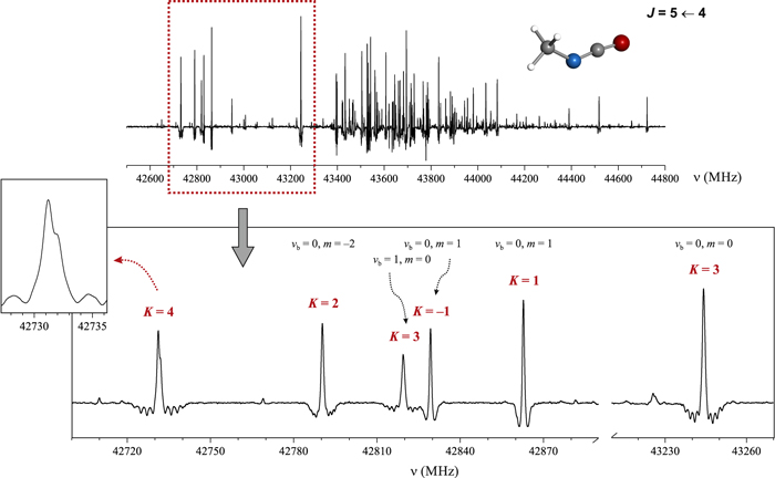
**Figure 1.** Top panel: CH₃NCO molecule and a section of the low-voltage, Stark-modulation spectrum (10 V) in the region of the $J=5\leftarrow 4$ rotational transition. Bottom panel and inset: detail of the spectrum showing a characteristic Stark effect and line shape asymmetry for isolated transitions. While K = 1 and K = 2 transitions are not well modulated, clear fast first-order Stark lobes (see the text) can be observed for the K = 3 transitions, and the increase of the Stark lobe span with K allows easy identification of the K = 4 transition. Furthermore, the line shape of the K = 4 transition is affected by the nuclear quadrupole hyperfine structure, which is in agreement with predictions in Figure 2.
Download figure:
Standard image High-resolution image

**Figure 1.** Top panel: CH₃NCO molecule and a section of the low-voltage, Stark-modulation spectrum (10 V) in the region of the $J=5\leftarrow 4$ rotational transition. Bottom panel and inset: detail of the spectrum showing a characteristic Stark effect and line shape asymmetry for isolated transitions. While K = 1 and K = 2 transitions are not well modulated, clear fast first-order Stark lobes (see the text) can be observed for the K = 3 transitions, and the increase of the Stark lobe span with K allows easy identification of the K = 4 transition. Furthermore, the line shape of the K = 4 transition is affected by the nuclear quadrupole hyperfine structure, which is in agreement with predictions in Figure 2.
Download figure:
Standard image High-resolution image

Another useful feature, observed in the lowest-J rotational spectra of CH₃NCO, is the nuclear quadrupole hyperfine structure due to the presence in the molecule of a single ¹⁴N nucleus. At the current resolution of the Stark spectra in Figure 1, this gives rise to a noticeable asymmetry in the line shapes for K = J'' transitions (as for the K = 4 line in Figure 1). As shown in Figure 2, these doublets can be better resolved in the frequency-modulated spectra not only for K = J'' but also for K = J'' − 1 transitions. The frequency splitting in the doublet is measurable and is compared in Figure 2 with predictions based on the most recent hyperfine splitting constants for CH₃NCO (Cernicharo et al. 2016). The hyperfine patterns thus provide independent confirmation of the assignments based on the Stark patterns. The behavior of the Stark and hyperfine patterns as a function of K and J'' for lines that are crucial to the higher-K assignment is further illustrated in Figure 3.

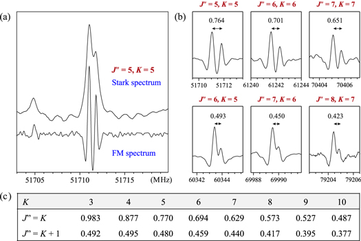
**Figure 2.** Line shapes for the higher-K transitions at the lowest possible values of J'' illustrating the characteristic, asymmetric doubling arising from the partially resolved nuclear quadrupole hyperfine structure. (a) Comparison of the resolution in Stark and frequency-modulated (FM) spectra. (b) Illustration of the relatively constant, resolvable doubling visible in FM spectra for the J'' = K lines, which decreases rapidly for J'' = K + 1 transitions. (c) Calculated values of the splitting to compare with the experimental values indicated in the previous panel.
Download figure:
Standard image High-resolution image

**Figure 3.** Diagram of Stark line shapes for some K = J'', K = J'' − 1, and K = J'' − 2 transitions showing the increasing frequency span of the Stark lobe pattern on increasing K for a given value of J'', while for a given K the width of the Stark pattern and the hyperfine splitting decrease rapidly with increasing J''.
Download figure:
Standard image High-resolution image

The application of these criteria and step-by-step inspection of spectral regions corresponding to higher-J transitions then allowed the identifications of K = 5–10 transitions. The availability of two different criteria was especially useful in the denser portions of the spectra, where the characteristic Stark lobes could not be clearly distinguished owing to overlaps with those of neighboring lines. Final confirmation of the K assignments was made simply by the absence of the corresponding lines in the spectral region for J < K. Once the K > 3 transitions were successfully assigned in the low-frequency Stark spectra for lowest J, their higher-J counterparts could be easily located in the higher-frequency spectra (up to 364 GHz) measured in our previous work (Cernicharo et al. 2016). Graphical Loomis–Wood-type plotting techniques as built into the AABS package (Kisiel et al. 2005, 2012) proved invaluable for this purpose. The J dependence of frequencies for a given set of K, m, and v_b quantum number values is a smooth function so that such transition sequences are readily identifiable.

Koput (1986) has shown that the global fitting of the rotational spectrum of CH₃NCO to experimental accuracy is an extremely challenging task. For this reason, the experimental spectrum has been broken down in our previous work into more than 220 (K, m, ${\upsilon }_{{\rm{b}}}$ ) sequences of correlated lines, with each sequence analyzed separately (see Cernicharo et al. 2016, for details). The same pragmatic approach is employed in this work. Each of the identified K > 3 sequences was thus fitted to a suitable linear-rotor-type J(J + 1) power series expansion for the rotational energies

$\begin{eqnarray}\begin{array}{rcl}{E}_{\mathrm{rot}} & = & {BJ}(J+1)-{D}_{J}{J}^{2}{\left(J+1\right)}^{2}+{H}_{J}{J}^{3}{\left(J+1\right)}^{3}\\ & & +{L}_{J}{J}^{4}{\left(J+1\right)}^{4}+{P}_{J}{J}^{5}{\left(J+1\right)}^{5}+{P}_{12}{J}^{6}{\left(J+1\right)}^{6}\\ & & +{P}_{14}{J}^{7}{\left(J+1\right)}^{7}+{P}_{16}{J}^{8}{\left(J+1\right)}^{8}+{P}_{18}{J}^{9}{\left(J+1\right)}^{9},\end{array}\end{eqnarray} \tag{ 1 }$

where the lengths of the centrifugal distortion expansions were established empirically. In cases of partially resolved nuclear quadrupole hyperfine structure, such as those in Figure 2, an intensity-weighed frequency average has been the measured frequency used in the fitting procedure. The determined linear-rotor-type parameters are listed in Table 1, while the experimental frequencies are collected in Table 2. It has to be noted that while the assignment of the K quantum numbers is confident, the assignment of m quantum numbers is rather uncertain, although a general decrease of intensity with increasing m may be expected. For this reason in Table 1 we list the sequences in order of decreasing intensity for each K and adopt a modified naming convention in relation to that used in Cernicharo et al. (2016). For example, for K = 4 transitions, the labeling of corresponding sequences is as follows: K4a, K4b, K4c, etc., where a, b, c are assigned in the order of decreasing relative intensity at room temperature (a strongest, b second strongest, etc.). Many sequences for K = 4 and 5 consist of degenerate lower-J parts, separating into two distinct series at high J. In such cases L and U letters are added (e.g., K4aL, K4aU) in order to distinguish between the components separating to lower and upper frequency, respectively. In some cases a line sequence displayed a J dependence of transition frequencies that was smooth but sufficiently nonlinear to fall outside the tractability as a whole with Equation (1). This necessitated splitting the sequence into two parts (with prefixes V and X), such as for the strongest K = 4 sequence in Table 1 reproduced by parts V129 and X129.

Table 1. Parameters of the Linear-rotor-type, J(J + 1) Power Series Fitted to the Assigned K > 3 Line Sequences of the Parent Species

K^a	Name^b	I_rel^c	N_in^d	N_rej^e	σ_w^f	B^g (MHz)	D_J (kHz)	H_J (Hz)	L_J (mHz)	P_J (μHz)	P₁₂ (nHz)	P₁₄ (pHz)	P₁₆ (fHz)	P₁₈ (aHz)
K = 4

K4aL	V129:		10	0	3.159	3830.2(86)	−8.74(32) × 10³	−1.295(64) × 10⁵	1.287(81) × 10⁶	−8.59(65) × 10⁶	3.79(33) × 10⁷	−1.05(10) × 10⁸	1.69(19) × 10⁸	−1.17(14) × 10⁸
	X129:	0.758	27	0	4.944	4200.20(73)	−121.8(37)	−305.(10)	404.(18)	-343.(19)	194.(13)	−70.0(58)	14.6(13)	−1.34(14)
K4aU	V130:		10	0	3.764	3834.(10)	−8.62(38) × 10³	−1.269(77) × 10⁵	1.255(96) × 10⁶	−8.33(77) × 10⁶	3.66(39) × 10⁷	−1.02(12) × 10⁸	1.62(22) × 10⁸	−1.12(17) × 10⁸
	X130:	0.759	27	0	4.904	4200.15(72)	−122.1(37)	−306.(10)	405.(18)	-345.(19)	195.(13)	−70.4(58)	14.7(13)	−1.35(14)
K4bL	V102:		9	0	0.0	4746.97	24.017 × 10³	6.163 × 10⁵	−11.571 × 10⁶	131.94 × 10⁶	−97.67 × 10⁷	45.165 × 10⁸	−1.1835 × 10¹⁰	1.34 × 10¹⁰
	X102:	0.734	29	0	2.597	4232.88 (10)	−7.18 (67)	18.5 (23)	−40.4 (47)	46.3 (60)	−32.9 (46)	14.4 (22)	−3.53(59)	0.373(66)
K4bU	V103:		9	0	0.254	4746.93 )	24.014 × 10³	6.152 × 10⁵	−11.568 × 10⁶	131.91 × 10⁶	−97.63 × 10⁷	45.145 × 10⁸	−1.1829 × 10¹⁰	1.34 × 10¹⁰
	X103:	0.737	29	0	1.349	4232.152(74)	−11.43(46)	5.7 (15)	−16.9 (30)	19.2 (36)	−13.2 (28)	5.6 (13)	−1.36(34)	0.141(38)
K4c	V004:	0.727	29	6	0.869	4346.5608(20)	1.536(10)	0.044(22)	−0.085(20)	0.0428(67)	⋯	⋯	⋯	⋯
K4dL	V141:	0.694	37	0	1.304	4405.4265(92)	41.59(12)	61.43(83)	−84.5(30)	96.7(62)	−81.1(79)	45.0(59)	−14.7(24)	2.12(42)
K4dU	V140:	0.714	37	0	0.914	4405.4441(68)	41.936(98)	64.27(67)	−96.4(25)	124.3(55)	−118.0(74)	73.7(58)	−26.7(25)	4.23(46)
K4e	V051:	0.547	37	0	1.228	4389.1854(20)	2.0690(67)	−0.1645(92)	0.1082(55)	−0.0216(12)	⋯	⋯	⋯	⋯
K4f	V108:	0.493	30	5	0.947	4365.1008(16)	1.9297(57)	−0.0254(79)	0.0123(47)	−0.0031(10)	⋯	⋯	⋯	⋯

K = 5

K5a	V022:	0.988	33	3	1.016	4365.4070(12)	2.2359(26)	0.0252(21)	−0.00129(56)	⋯	⋯	⋯	⋯	⋯
K5bL	V109:	0.714	31	4	1.192	4306.3355(75)	−43.955(76)	−57.56(37)	81.49(96)	−89.8(15)	73.7(14)	−39.45(76)	11.69(23)	−1.438(29)
K5bU	V110:	0.701	31	3	0.932	4306.3197(62)	−44.176(67)	−58.88(34)	85.54(96)	−96.9(16)	81.2(15)	−43.93(90)	13.11(28)	−1.623(38)
K5c	V001:	0.676	35	0	1.240	4350.4222(15)	1.4947(31)	0.0136(25)	0.00635(66)	⋯	⋯	⋯	⋯	⋯
K5d	V092:	0.573	36	1	1.030	4341.4381(58)	6.558(55)	−2.24(25)	1.08(61)	−4.27(89)	5.22(78)	−3.97(40)	1.58(11)	−0.239(13)
K5e	V062:	0.441	34	0	1.260	4399.9696(15)	2.2318(32)	−0.0084(25)	−0.00105(68)	⋯	⋯	⋯	⋯	⋯
K5f	V049:	0.427	26	1	1.282	4387.7577(25)	2.0469(83)	−0.085(12)	0.0435(70)	−0.0082(15)	⋯	⋯	⋯	⋯
K5g	V122:	0.336	29	0	1.201	4355.8543(52)	−2.796(35)	1.06(11)	1.02(17)	0.73(15)	−0.998(64)	0.226(11)	⋯	⋯
K5h	V087:	0.269	32	1	0.993	4354.3392(12)	1.6359(25)	−0.0057(21)	0.00323(56)	⋯	⋯	⋯	⋯	⋯
K5iL	V238:	0.179	29	0	0.833	4356.1661(32)	−0.481(20)	0.319(55)	0.698(80)	−0.082(63)	−0.097(25)	0.0204(40)	⋯	⋯
K5iU	V239:	0.172	30	0	0.916	4356.1725(35)	−0.424(22)	0.525(62)	0.350(89)	0.210(68)	−0.213(27)	0.0382(42)	⋯	⋯

K = 6

K6a	V009:	1.000	32	3	1.291	4353.4867(16)	0.5959(33)	−0.0358(26)	0.02590(70)	⋯	⋯	⋯	⋯	⋯
K6b	V036:	0.834	34	0	0.849	4374.6209(10)	2.0963(21)	0.0021(17)	0.00123(45)	⋯	⋯	⋯	⋯	⋯
K6c	V011:	0.592	32	2	0.874	4355.09118(70)	1.89726(79)	−0.00678(26)	⋯	⋯	⋯		⋯	⋯
K6d	V003:	0.507	34	0	1.036	4347.7439(26)	0.378(12)	0.335(25)	−0.152(25)	−0.110(11)	0.0335(21)	⋯	⋯	⋯
K6e	V233:	0.492	27	0	0.967	4412.075(14)	−5.10(20)	13.6(13)	9.3(52)	88.(11)	−286.(16)	311.(13)	−152.0(59)	28.8(11)
K6f	V048:	0.344	31	2	0.942	4386.55941(80)	2.06674(93)	0.00262(32)	⋯	⋯	⋯	⋯	⋯	⋯
K6g	V184:	0.312	24	3	1.206	4411.8773(63)	1.884(55)	−0.46(21)	1.09(44)	−1.49(50)	1.03(28)	−0.284(64)	⋯	⋯
K6h	V145:	0.311	29	3	1.121	4388.1291(45)	2.313(27)	0.091(78)	−0.24(11)	0.287(90)	−0.160(35)	0.0314(56)	⋯	⋯
K6i	V061:	0.227	27	8	1.208	4399.4906(12)	2.1265(13)	0.00638(43)	⋯	⋯	⋯	⋯	⋯	⋯
K6j	V064:	0.146	32	2	0.805	4401.17868(65)	2.13354(74)	0.00560(24)	⋯	⋯	⋯	⋯	⋯	⋯
K6k	V078:	0.099	30	1	1.069	4426.54770(94)	2.2099(10)	0.00665(34)	⋯	⋯	⋯	⋯	⋯	⋯

K = 7

K7a	V013:	0.892	31	3	1.108	4357.7248(14)	1.6500(30)	−0.0152(23)	0.00193(62)	⋯	⋯	⋯	⋯	⋯
K7b	V123:	0.388	30	2	1.280	4364.1594(10)	1.8941(12)	−0.00551(40)	⋯	⋯	⋯	⋯	⋯	⋯
K7c	V084:	0.342	27	4	0.839	4360.3493(12)	0.8838(24)	−0.1255(19)	0.01255(49)	⋯	⋯	⋯	⋯	⋯
K7d	V063:	0.278	31	1	0.875	4400.6256(28)	2.318(13)	0.153(27)	−0.008(28)	−0.061(13)	0.0192(26)	⋯	⋯	⋯
K7e	V060:	0.245	30	1	1.140	4398.34077(98)	2.1058(11)	0.00548(36)	⋯	⋯	⋯	⋯	⋯	⋯
K7f	V077:	0.229	32	0	0.734	4425.4453(10)	2.1866(20)	0.0030(15)	0.00108(41)	⋯	⋯	⋯	⋯	⋯
K7g	V069:	0.166	33	1	1.114	4411.64576(89)	2.1514(10)	0.00692(33)	⋯	⋯	⋯	⋯	⋯	⋯

K = 8

K8a	V021:	0.682	26	2	0.960	4364.1271(15)	1.9735(30)	−0.0069(23)	−0.00255(61)	⋯	⋯	⋯	⋯	⋯
K8b	V059:	0.491	31	2	1.242	4397.4177(17)	2.1423(34)	0.0089(27)	−0.00519(71)	⋯	⋯	⋯	⋯	⋯
K8c	V174:	0.380	31	1	1.303	4389.7174(45)	1.802(19)	0.453(38)	−0.382(36)	0.417(17)	−0.0919(30)	⋯	⋯	⋯
K8d	V194:	0.296	18	1	1.154	4361.0443(33)	0.6630(93)	0.029(11)	0.0788(68)	−0.0091(14)	⋯	⋯	⋯	⋯

K = 9

K9a	V165:	0.495	28	3	1.097	4373.1956(44)	−1.075(18)	0.213(35)	0.059(33)	0.085(15)	−0.0336(27)
K9b	V068:	0.375	29	2	0.917	4409.55603(80)	2.13686(88)	0.00221(29)	⋯	⋯	⋯	⋯	⋯	⋯
K9c	V152:	0.261	25	1	0.829	4377.4805(12)	1.6836(26)	−0.0156(20)	0.00197(53)	⋯	⋯	⋯	⋯	⋯
K9d	V035:	0.282	27	2	1.073	4373.4274(16)	2.0711(32)	0.0191(25)	0.00245(65)	⋯	⋯	⋯	⋯	⋯
K9e	V034:	0.146	25	3	1.331	4372.0337(12)	2.0403(14)	0.00960(48)	⋯	⋯	⋯	⋯	⋯	⋯
K9f	V200:	0.105	26	3	1.262	4396.09603(60)	2.01705(26)	⋯	⋯	⋯	⋯	⋯	⋯	⋯

K = 10

K10a	V027:	0.393	27	3	1.196	4367.2143(19)	1.4495(38)	0.0095(30)	0.00302(79)	⋯	⋯	⋯	⋯	⋯
K10b	V074:	0.241	27	2	1.062	4422.1124(10)	2.1495(11)	0.00574(38)	⋯	⋯	⋯	⋯	⋯	⋯
K10c	V173:	0.188	29	0	1.425	4392.41226(90)	1.98881(28)	⋯	⋯	⋯	⋯	⋯	⋯	⋯

Notes.

^aThe notation of individual K sequences as described in the text following Equation (1). ^bThe identifier of the line sequence established in Cernicharo et al. (2016). ^cAutomatically assigned intensity of the sequence relative to the strongest sequence in the spectrum. ^dThe number of lines in the linear fit. ^eThe number of confidently assigned lines that were perturbed and were rejected from the fit. ^fUnitless (weighted) deviation of the effective rotor fit. ^gThe values of the parameters resulting from the effective linear-rotor fit.

Download table as: ASCIITypeset images: 1 2

Table 2. Line List of K > 3 Rotational Transitions for CH₃NCO Compiled from Experimental Frequencies (MHz) Assigned on the Basis of Stark-modulation Spectroscopy and Nuclear Quadrupole Hyperfine Structure

	K = 4
J'	J''	K4aL^a	K4aU	K4bL	K4bU	K4c	K4dL	K4dU	K4e	K4f
5	4	⋯^b	⋯^b	42731.292^c	42731.292^c	43464.849^c	44034.686^c	44034.686^c	43890.896^c	43650.061^c
6	5	⋯^b	⋯^b	50964.759	50964.759	52157.325^c	52831.945^c	52831.945^c	52668.393^c	52379.568^c
7	6	58339.391	58339.391	59350.121	59350.121	60849.700	61624.560	61624.560	61445.688	61108.737
8	7	66984.159	66984.159	67783.970	67783.970	69541.847	70412.420	70412.420	70222.650	69837.656
9	8	75576.792	75576.792	76238.725	76238.725	78233.684	79195.280	79195.280	78999.235	78566.221
10	9	84141.319	84141.319	84705.058	84705.058	86925.110	87973.153	87973.153	87775.326	87294.305
Sequence		V129+X129	V130+X130	V102+X102	V103+X103	V004	V141+X141	V140+X140	V051	V108

Notes. All frequencies (unless otherwise marked) are experimental measurements with estimated uncertainty of 0.05 MHz.

^aThe sequence notation as specified in the text. ^bTransition for which there is no experimental value and the extrapolation from a polynomial fit is not reliable. ^cIntensity-weighted average of the hyperfine doublet. (This table is available in its entirety in FITS format.)

Download table as: ASCII Typeset image

Apart from the K > 3 transitions, a comprehensive investigation of the Stark spectra made it possible to assign also some K ≤ 3 transitions in the v_b = 0 state of the parent isotopic species, such as K = −2, m = 1 or K = −1, m = 3L, that were missing in our preceding paper and that are expected to result in identifiable spectral features in the interstellar line surveys. Attempts were made to locate also K = −2, m = −2; K = −2, m = 3L; and K = −2, m = 3U sequences of transitions; however, they seem to be strongly perturbed. For completeness, K ≤ 3 transition sequences in the higher-energy m = 4, −5, and 6 internal rotor states of v_b = 0, assigned by Koput (1986), were also extended into the millimeter-wave region. Ultimately, several K ≤ 3 sequences of transitions could also be identified in v_b = 1 and v_b = 2 excited vibrational states as shown in Figure 4. For all these K < 3 transitions we follow the notation from Cernicharo et al. (2016). In the case of the m = 0 state, for which asymmetric rotor notation K_a and K_c would normally be more appropriate, we use the notation K = nL, nU to distinguish between lower (K_a + K_c = J + 1) and upper (K_a + K_c = J) frequency sequences for the same value of K_a = n. Analogously, we use the notation m = 3L and 3U to distinguish between the two nearly degenerate m = 3 substates giving rise to lower and upper frequency transition sequences, respectively. Although in the foreseeable future astrophysical detection of lines corresponding to these higher vibrational energy states appears more challenging, it cannot be completely discounted as shown recently by detection of several lines of CH₃NCO in v_b = 1 toward Sgr B2(N2) (Belloche et al. 2017). The sets of parameters of the linear-rotor-type, J(J + 1) power series for all these additionally assigned K ≤ 3 sequences are given in Table 3, and the experimental frequencies are gathered in Table 4 . Finally, the JPL catalog line list for these sequences is provided in Table 5.

**Figure 4.** Typical Stark pattern (10 V modulation voltage) observed for the m = 0, K_a = 2 asymmetry doublet in the ground state v_b = 0 and two successive excitations of the CNC bending mode v_b = 1 and v_b = 2. The irregular frequency progression of the three marked doublets is indicative of the anharmonicity/perturbations in the CNC bending motion.
Download figure:
Standard image High-resolution image

Table 3. Parameters of the Linear-rotor-type, J(J + 1) Power Series Fitted to the Additionally Assigned K ≤ 3 Line Sequences of the Parent Species

K^a	Name^b	I_rel^c	N_in^d	N_rej^e	σ_w^f	B (MHz)	D_J (kHz)	H_J (Hz)	L_J (mHz)	P_J (μHz)	P₁₂ (nHz)	P₁₄ (pHz)	P₁₆ (fHz)	P₁₈ (aHz)
${\upsilon }_{{\rm{b}}}=0$ , m = 1 E: E_vib = 8.4 cm⁻¹
−2a	V179:	0.579	16	1	0.494	4350.3325(51)	−78.80(10)	−44.0(10)	−238.0(46)	526.(10)	−356.5(84)	⋯	⋯	⋯
−2b	X179:	0.789	22	0	1.016	4344.71(97)	−125.0(46)	−253.(12)	309.(20)	−260.(21)	149.(14)	−55.4(64)	12.1(15)	−1.16(16)
${\upsilon }_{{\rm{b}}}=0$ , m = 3 U $(K=0,J=1,0={A}_{2},{A}_{1})$ : ${E}_{\mathrm{vib}}=79.7$ cm⁻¹
−1	V138:	0.663	34	5	1.577	4377.4365(70)	−10.872(77)	3.73(40)	−27.1(11)	24.8(17)	−20.7(16)	13.66(90)	−4.81(27)	0.658(34)
${\upsilon }_{{\rm{b}}}=0$ , m = 4 E: E_vib = 140.6 cm⁻¹
−1	V164:	0.502	36	3	1.259	4372.7579(28)	−0.421(13)	0.001(29)	0.560(30)	−0.246(14)	0.0193(27)	⋯	⋯	⋯
1	V160:	0.312	29	1	1.076	4372.9957(46)	1.714(48)	−1.04(23)	2.72(56)	−4.08(74)	3.13(48)	−0.97(12)	⋯	⋯
−2	V229:	0.461	26	0	1.183	4407.0035(81)	−23.20(14)	87.6(12)	−344.4(54)	243.(13)	145.(18)	−259.(13)	93.4(41)	⋯
2	V158:	0.209	34	5	1.213	4379.0786(10)	2.0825(11)	−0.00046(37)	⋯	⋯	⋯	⋯	⋯	⋯
2'	V159:	0.209	34	5	1.404	4379.0839(17)	2.1043(38)	0.0111(33)	−0.01225(93)	⋯	⋯	⋯	⋯	⋯
${\upsilon }_{{\rm{b}}}=0$ , m = −5 E: E_vib = 217.5 cm⁻¹
−1	V045:	0.252	34	2	0.854	4384.15287(41)	2.11044(22)	⋯	⋯	⋯	⋯	⋯	⋯	⋯
2	V193:	0.413	37	2	0.994	4388.1800(34)	−2.184(29)	1.09(11)	−0.28(23)	1.74(27)	−1.84(17)	0.608(61)	−0.0661(86)	⋯
−2	V056:	0.199	38	1	0.961	4393.35137(72)	2.17888(83)	0.00628(28)	⋯	⋯	⋯	⋯	⋯	⋯
${\upsilon }_{{\rm{b}}}=0$ , m = 6 A: E_vib = 311.1 cm⁻¹
0	V175:	0.377	35	3	1.248	4387.7938(21)	2.1700(70)	0.0974(97)	−0.0479(58)	0.0092(13)	⋯	⋯	⋯	⋯
−1	V136:	0.458	35	4	1.089	4383.39713(85)	1.89120(97)	0.00489(33)	⋯	⋯	⋯	⋯	⋯	⋯
1	V058:	0.314	40	0	1.023	4395.72730(75)	2.19786(86)	0.00391(29)	⋯	⋯	⋯	⋯	⋯	⋯
−2	V147:	0.533	37	2	1.054	4386.2913(12)	0.8694(25)	0.0705(20)	0.02113(54)	⋯	⋯	⋯	⋯	⋯
${\upsilon }_{{\rm{b}}}=1$ , m = 0: E_vib = 182.2 cm⁻¹
2L	V090:	0.356	36	3	1.077	4342.2441(23)	3.281(11)	0.144(24)	−0.118(24)	0.062(11)	−0.0124(22)	⋯	⋯	⋯
2U	V088:	0.385	38	1	1.054	4342.2228(12)	−2.0956(25)	−0.1958(20)	−0.02294(53)	⋯	⋯	⋯	⋯	⋯
3L	V104:	0.339	32	5	0.852	4282.6194(34)	13.690(30)	7.53(11)	2.05(21)	−4.58(22)	2.59(13)	−0.707(44)	0.0790(58)	⋯
3U	V105:	0.325	31	6	0.991	4282.6294(41)	13.818(39)	8.01(14)	1.27(27)	−3.85(28)	2.20(17)	−0.593(55)	0.0653(72)	⋯
${\upsilon }_{{\rm{b}}}=1$ , m = 1: E_vib = 191.4 cm⁻¹
0a	V177:		21	0	0.774	4353.3169(60)	122.30(14)	37.3(16)	429.6(88)	−1143.(25)	1306.(37)	−593.(21)	⋯	⋯
0b	X177:	0.359	15	0	0.703	4357.44(27)	164.3(13)	264.3(34)	−288.8(52)	202.9(47)	−83.0(22)	15.02(45)	⋯	⋯
−1	V099:	0.379	39	2	1.147	4294.0094(36)	−19.616(29)	−19.36(11)	14.63(21)	−8.80(24)	3.63(15)	−0.883(50)	0.0942(66)	⋯
${\upsilon }_{{\rm{b}}}=1$ , m = −2: E_vib = 222.3 cm⁻¹
0	V120:	0.345	38	2	0.838	4355.3770(22)	0.539(15)	0.556(44)	−1.554(66)	0.086(52)	0.190(21)	−0.0384(33)	⋯	⋯
−1	V015:	0.270	32	4	0.938	4357.25912(76)	1.43704(90)	−0.00953(30)	⋯	⋯	⋯	⋯	⋯	⋯
${\upsilon }_{{\rm{b}}}=2$ , m = 0: E_vib = 357.9 cm⁻¹
0	V095:	0.187	41	1	0.740	4330.7106(23)	6.917(19)	0.415(70)	−0.42(13)	0.50(15)	−0.316(96)	0.102(31)	−0.0134(42)	⋯
1L	V128:	0.176	38	2	1.180	4294.05621(88)	3.05470(94)	0.07787(30)	⋯	⋯	⋯	⋯	⋯	⋯
1U	V217:	0.156	31	2	1.139	4375.67247(93)	4.1429(10)	0.03510(37)	⋯	⋯	⋯	⋯	⋯	⋯
2L	V091:	0.156	31	4	1.263	4343.4842(16)	3.1549(33)	0.0395(26)	−0.00193(70)	⋯	⋯	⋯	⋯	⋯
2U	V113:	0.172	33	4	1.091	4343.4743(13)	−1.0207(27)	−0.1855(22)	−0.01014(59)	⋯	⋯	⋯	⋯	⋯

Notes.

^aThe value of the K_a or K quantum number following the notation described in Cernicharo et al. (2016). ^bThe identifier of the line sequence established in Cernicharo et al. (2016). ^cAutomatically assigned intensity of the sequence relative to the strongest sequence in the spectrum. ^dThe number of lines in the linear fit. ^eThe number of confidently assigned lines that were perturbed and were rejected from the fit. ^fUnitless (weighted) deviation of the fit.

Download table as: ASCII Typeset image

Table 4. Line List of Rotational Transitions for CH₃NCO Compiled from Experimental Frequencies (MHz) for Additional K ≤ 3 Line Sequences Assigned on the Basis of Continuity from the Assignment Reached by Koput (1986) for J'' ≤ 3

${\upsilon }_{b}=0$ , m = 4, E_vib = 140.6 cm⁻¹^a
J'	J''	K = −1^a	K = 1	K = −2	K = 2
2	1	17491.620^b	17491.620^b	⋯	⋯
3	2	26236.710^b	26237.850^b	26444.570^b	26274.290^b
4	3	34982.163	34983.529	35262.419	35032.080
5	4	43727.872	43729.167	44083.027	43789.693
6	5	52473.515	52474.398	52907.508	52547.163
7	6	61219.189^c	61219.500^c	61736.631	61304.239
8	7	69965.011	69964.211	70571.424	70060.972
Sequence^a		V164	V160	V229	V158

Notes. All frequencies (unless otherwise marked) are hyperfine-free experimental measurements with estimated uncertainty of 0.05 MHz.

^aThe vibrational energies, K quantum number, and sequence notations are the same as in Cernicharo et al. (2016). ^bTaken from Koput (1986). ^cCalculated from a J(J + 1) power series fit to the sequence (mainly due to line blending). (This table is available in its entirety in FITS format.)

Download table as: ASCII Typeset image

Table 5. JPL Catalog Line List for Additional K ≤ 3 Transitions of CH₃NCO

Frequency	Error	Log(Int)^a	DR^b	E_low	g_upp^c	TAG^d	QNFMT^e	QN'^f					QN''^g
(MHz)	(MHz)			(cm⁻¹)				J'	${K}_{a}^{{\prime} }$	${K}_{c}^{{\prime} }$	$m^{\prime}$	${\upsilon }_{{\rm{b}}}^{{\prime} }$	$J^{\prime\prime}$	${K}_{a}^{{\prime\prime} }$	${K}_{c}^{{\prime\prime} }$	$m^{\prime\prime}$	${\upsilon }_{{\rm{b}}}^{{\prime\prime} }$
61299.229	0.0500	−5.1774	3	89.9688	15	01	505	7	−1	0	3	0	6	−1	0	3	0
70061.612	0.0500	−5.0059	3	92.0119	17	01	505	8	−1	0	3	0	7	−1	0	3	0
78825.997	0.0500	−4.8562	3	94.3469	19	01	505	9	−1	0	3	0	8	−1	0	3	0
87592.559	0.0500	−4.7237	3	96.9736	21	01	505	10	−1	0	3	0	9	−1	0	3	0
96361.445	0.0500	−4.6051	3	99.8922	23	01	505	11	−1	0	3	0	10	−1	0	3	0
105132.553	0.0500	−4.4982	3	103.1026	25	01	505	12	−1	0	3	0	11	−1	0	3	0

Notes. The key parameters used in the evaluation of this table, μ = μ_a = 2.882 D, T = 300 K, and Q_vr = 138,369, are defined in Sections A.1 and A.2 of Cernicharo et al. (2016).

^aBase-10 logarithm of the integrated intensity at 300 K in units of nm² MHz. ^bDegrees of freedom in the rotational partition function. ^cUpper-state degeneracy. ^dSpecies tag or molecular identifier. ^eFormat of the quantum numbers. ^fQuantum numbers for the upper state. K_a and K_c quantum numbers are defined only for the m = 0 state. For m > 0: K_a = K and K_c = 0. ^gQuantum numbers for the lower state. K_a and K_c quantum numbers are defined only for the m = 0 state. For m > 0: K_a = K and K_c = 0.

Only a portion of this table is shown here to demonstrate its form and content. A machine-readable version of the full table is available.

Download table as: Data Typeset image

A useful overview of the features hindering the solution of the spectroscopic problem for CH₃NCO is provided in Figure 5. In this reduced frequency representation based on Equation (1) the sequences are expected to converge at low J to the effective values of B as tabulated in Tables 1 and 3. Only moderate (and uniform) curvature in the vertical direction is expected. A useful reference is provided by the quasi-linear NCNCS molecule (see Figure 8 of Winnewisser et al. 2010). For NCNCS the behavior appears to be less perturbed than that visible in Figure 5, but in that case reproduction of the rotational spectrum to within experimental accuracy has not yet been achieved. In the present case of CH₃NCO the situation is considerably more complex since the most important, lowest-K sequences in the lowest internal rotation substates m = 0 and 1 appear to show the most unusual behavior. The m = 0, K = 3 sequence is already significantly shifted to low frequency relative to limited fits made with the standard asymmetric rotor model (as reproduced in the discussion of the ¹³C species further below). Furthermore, the most intense K = 4 sequence, and thus the first candidate to be assigned to m = 0, is displaced even more to low frequency and is highly nonlinear. It is only at higher K where the sequences are closer to the positions expected from standard asymmetric rotor theory, but their ordering is by no means regular. The behavior of the m = 1 sequences as assigned by Koput (1986), in particular of that for K = 0, is also very challenging. In principle, low barrier methyl group internal rotation is treatable with the RAM36 program of Ilyushin et al. (2010). The program has been very successful in treating toluene, which is a molecule with a very similar energy distribution of internal rotor states to that in CH₃NCO, and also displaying a plethora of perturbations between m = 0 and 1 substates (Ilyushin et al. 2017). In fact, RAM36 has already been applied to CH₃NCO (Halfen et al. 2015), albeit to a very small data set, which has later been shown to contain some misassignments (Cernicharo et al. 2016). The reported predictions allowed confident assignment in Sagittarius B2 of some conservatively chosen CH₃NCO transitions (Halfen et al. 2015) but turned out to be of a very limited character when confronted with the complete laboratory data (Cernicharo et al. 2016). The currently available data set is being used to reach a more comprehensive RAM36 fit. Progress is slow, one of the reasons being that multiple competing parameters of fit are involved. The choice of numerical values of even the leading parameters defining internal rotation for this low barrier case, such as ρ, F, V₃, D_ab, and Q_b (see Lin & Swalen 1959) is already found to be critical. Their values can be precalculated with moderate confidence, but in order to reach spectroscopic accuracy, each such parameter also needs to be supported by an associated centrifugal-type expansion, which is much more poorly understood. Furthermore, the J dependence of the observed line sequences also lacks the sharp resonances that allow precise identification of the positions of interacting vibration–rotation energy levels (as has been the case for toluene; Ilyushin et al. 2017). For the time being we prefer to make the extensive laboratory data available for applications and to cite Curl et al. (1963), who, on being confronted with the CH₃NCO spectrum, stated, "There seems to be little value in reporting values of the constants obtained or details of the fits." Nevertheless, the analysis in terms of transition series of the complete rotational spectrum of CH₃NCO up to 364 GHz allows approximate estimation of most of the rovibrational energy levels within 400 cm⁻¹ or so from J = 0 of the ground state with E_vr ( cm⁻¹) = 0.14462 $J(J+1)+4.138{K}^{2}+{E}_{\mathrm{vib}}(m,{v}_{b})$ , where the two numerical constants are, respectively, (B + C)/2 and A − (B + C)/2 (from Cernicharo et al. 2016) and ${E}_{\mathrm{vib}}(m,{v}_{b})$ are the vibrational substate energies from Koput (1986).

**Figure 5.** Illustration of the complexity underlying the rotational spectrum of CH₃NCO as revealed by a reduced frequency plot of identified transition sequences. In this representation transition series for a "well-behaved" molecule are expected to show only relatively small curvature from the vertical, such as on the right side of the figure. This is clearly not the case for many important series. Color-coding: red—the lowest-K ground-state (m = 0) sequences; blue—the lowest- $K\,m=1$ sequences; black—the most intense sequences for each value of K for the currently assigned K > 3 series; green—the remaining currently assigned K > 3 series; gray—other series. The values of K for selected series are indicated.
Download figure:
Standard image High-resolution image

3.2. ¹³C Isotopic Species

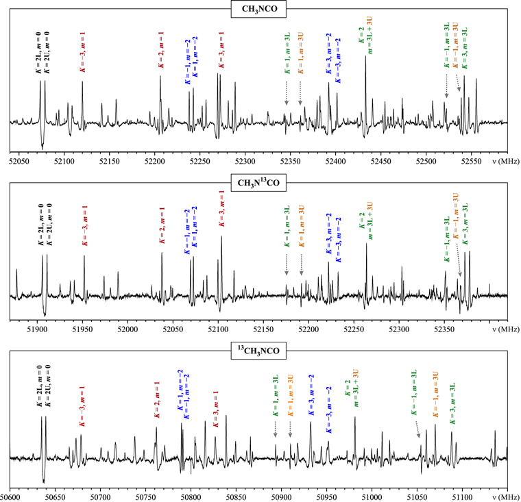
Three different spectroscopic techniques were used for the assignment of rotational transitions of CH₃N¹³CO and ¹³CH₃NCO isotopologues. In a first step, their rotational signatures were searched for in natural abundance in the broadband chirped-pulse Fourier transform microwave spectrum (6–18 GHz and 25–26 GHz) acquired in our previous study (Cernicharo et al. 2016). This made possible the assignment of K_a = 0, m = 0, ${\upsilon }_{{\rm{b}}}=0$ lines solely on the basis of predicted frequency shifts induced by isotopic substitution. In a next step, Stark-modulation spectroscopy on isotopically enriched samples was used to discriminate between transitions with different values of the K quantum number. The assignments of m and ${\upsilon }_{{\rm{b}}}$ quantum numbers were subsequently transferred from the parent species on the basis of similarities of spectral patterns for corresponding J regions (see Figure 6). Finally, the assigned sequences were extended into the millimeter-wave range. The isocyanate carbon atom is very close to the center of mass of CH₃NCO, so that the $J=6\leftarrow 5$ spectrum of CH₃N¹³CO is shifted to low frequency by only ∼170 MHz. The effect on the line pattern in Figure 6 is seen to be minimal, so that quantum number assignment is readily transferable from the parent species. For ¹³CH₃NCO the corresponding isotopic frequency shift is ∼1440 MHz, and changes in the line pattern are seen to be more significant. Nevertheless, the key lines are also assignable on the basis of Stark behavior and relative intensity. The experimental line lists for the assigned transition sequences of CH₃N¹³CO and ¹³CH₃NCO with the lowest vibrational energies that are expected to be key in future astrophysical identifications are given in Tables 6 and 7. The labeling of the individual sequences, as well as the quantum number nomenclature, is kept the same as for the parent species. Similarly to the parent species, only K_a = 0, 1, 2, m = 0, ${\upsilon }_{{\rm{b}}}=0$ transitions could be fitted together with reasonable terms in Watson's semirigid asymmetric rotor Hamiltonian. Results of such fits are given in Tables 8 and 9. Table 10 then summarizes the spectroscopic parameters for each of the identified line sequences of CH₃N¹³CO and ¹³CH₃NCO obtained from the linear-rotor fits to Equation (1). The similarities in their values to those for the parent species as compared in Table 10 corroborate the correct assignments. The JPL catalog line lists for CH₃N¹³CO and ¹³CH₃NCO that are most directly useful for astrophysical applications are reported in Tables 11 and 12, respectively.

**Figure 6.** Stark spectra of the $J=6\leftarrow 5$ region for the parent and the two ¹³C isotopic species of CH₃NCO measured at modulation voltage of 10 V, with frequency axes aligned in a way highlighting the relatively small isotopic variation of the observed spectroscopic patterns. Comparison of the two top spectra gives evidence for the achieved high isotopic purity since no lines of the parent species are visible in the spectrum of CH₃N¹³CO.
Download figure:
Standard image High-resolution image

**Figure 6.** Stark spectra of the $J=6\leftarrow 5$ region for the parent and the two ¹³C isotopic species of CH₃NCO measured at modulation voltage of 10 V, with frequency axes aligned in a way highlighting the relatively small isotopic variation of the observed spectroscopic patterns. Comparison of the two top spectra gives evidence for the achieved high isotopic purity since no lines of the parent species are visible in the spectrum of CH₃N¹³CO.
Download figure:
Standard image High-resolution image

Table 6. Line List of Rotational Transitions for CH₃N¹³CO Compiled from Experimental Frequencies (MHz) for Line Sequences Assigned on the Basis of CP-FTMW, Stark-modulated, and Frequency-modulated Millimeter-wave Spectra

${\upsilon }_{b}=0$ , m = 0 (Ground State), E_vib = 0 cm⁻¹^a
J'	J''	K = 0^a	K = 1L	K = 1U	K = 2L	K = 2U	K = 3L	K = 3U
6	5	51853.337	51403.416	52340.000	51905.699	51910.851	51726.586	51726.586
7	6	60492.530	59969.439	61061.832	60555.431	60563.705	60345.859	60345.859
8	7	69130.253	68534.899	69782.881	69204.658	69217.015	68964.201	68964.201
9	8	77766.490	77099.721	78503.174	77853.205	77870.697	77581.512	77581.512
10	9	86400.869^b	85663.778	87222.481	86501.119	86525.020	86197.856	86197.856
11	10	95033.255^b	94227.186^b	95940.874^b	95148.303^b	95180.269^b	94812.773^b	94812.852^b
12	11	103663.458^b	102789.647^b	104658.087^b	103794.561^b	103836.065^b	103426.398^b	103426.526^b
Sequence^a		V093	V126	V131	V089	V006	V096	V097

Notes. All frequencies (unless otherwise marked) are hyperfine-free experimental measurements with estimated uncertainty of 0.05 MHz.

^aThe vibrational energies, K quantum number notation, and the labeling of the individual line sequences are the same as for the parent species in Cernicharo et al. (2016). ^bCalculated from a J(J + 1) power series fit to the sequence (interpolation due to line blending or missing data). (This table is available in its entirety in FITS format.)

Download table as: ASCII Typeset image

Table 7. Line List of Rotational Transitions for ¹³CH₃NCO Compiled from Experimental Frequencies (MHz) for Line Sequences Assigned on the Basis of CP-FTMW, Stark-modulated, and Frequency-modulated Millimeter-wave Spectra

${\upsilon }_{b}=0$ , m = 0 (Ground State), E_vib = 0 cm⁻¹^a
J'	J''	K = 0^a	K = 1L	K = 1U	K = 2L	K = 2U	K = 3L	K = 3U
6	5	50583.272	50151.340	51050.741	50634.955	50639.578	50482.694	50482.694
7	6	59010.994	58508.723	59557.732	59072.857	59080.538	58894.756	58894.756
8	7	67437.329	66865.576	68064.121	67510.342	67521.855	67306.163	67306.163
9	8	75862.078	75221.855	76569.588	75947.215	75963.479	75716.641	75716.641
10	9	84285.279^b	83577.376	85074.249	84383.466	84405.827	84126.212	84126.212
11	10	92706.543	91932.271^b	93577.977^b	92818.970^b	92848.738^b	92534.703^b	92534.775^b
12	11	101125.795	100286.312	102080.644	101253.657	101292.289	100942.013	100942.013
Sequence^a		V093	V126	V131	V089	V006	V096	V097

Notes. All frequencies (unless otherwise marked) are hyperfine-free experimental measurements with estimated uncertainty of 0.05 MHz.

^aThe vibrational energies, K quantum number notation, and the labeling of the individual line sequences are the same as for the parent species in Cernicharo et al. (2016). ^bCalculated from a J(J + 1) power series fit to the sequence (interpolation due to line blending or missing data). (This table is available in its entirety in FITS format.)

Download table as: ASCII Typeset image

Table 8. Spectroscopic Constants for the Ground States ( ${\upsilon }_{{\rm{b}}}=0$ , m = 0) of CH₃N¹³CO and ¹³CH₃NCO in Comparison with the Parent Species

Constant	Parent Species^a	CH₃N¹³CO	¹³CH₃NCO
A (MHz)	128435.(19)	128324.7(39)	127110.(25)
B (MHz)	4414.6182(93)	4400.1847(12)	4291.1542(90)
C (MHz)	4256.7490(85)	4243.2158(11)	4140.4916(82)
Δ_J (kHz)	2.3209(11)	2.30880(17)	2.22320(57)
Δ_JK (kHz)	−1274.0(13)	−1273.73(12)	−1240.5(14)
δ_J (kHz)	0.4042(14)	0.40068(25)	0.37712(92)
δ_K (kHz)	183.1(43)	[183.1]^b	160.8(41)
${{\rm{\Phi }}}_{J}$ (Hz)	−0.00191(47)	[−0.00191]^b	[−0.00191]^b
Φ_JK (Hz)	−5.39(24)	[−5.39]^b	−4.08(33)
${{\rm{\Phi }}}_{{KJ}}$ (Hz)	−68478.(285)	[−68478.]^b	−63001.(300)
ϕ_JK (Hz)	−47.6(14)	[−47.61]^b	−44.94(78)
N_lines^c	201	160	161
σ_fit^d (kHz)	94.6	88.5	99.6
σ_w^e	1.89	1.77	1.99

Notes. Numbers in parentheses are standard errors in units of the last digit.

^aTaken from Cernicharo et al. (2016). ^bFixed to the parent species value. ^cThe number of fitted lines. ^dStandard deviation of the fit. ^eUnitless (weighted) deviation of the fit.

Download table as: ASCII Typeset image

Table 9. Results of Fitting the Spectroscopic Constants of Table 8 for CH₃N¹³CO and ¹³CH₃NCO Ground States ( ${\upsilon }_{{\rm{b}}}=0$ , m = 0)

CH₃N¹³CO									¹³CH₃NCO
J'	${K}_{a}^{{\prime} }$	${K}_{c}^{{\prime} }$	$J^{\prime\prime}$	${K}_{a}^{{\prime\prime} }$	${K}_{c}^{{\prime\prime} }$	Obs.^a	O. – C.^b	Unc.^c	J'	${K}_{a}^{{\prime} }$	${K}_{c}^{{\prime} }$	J''	${K}_{a}^{{\prime\prime} }$	${K}_{c}^{{\prime\prime} }$	Obs.^a	O. – C.^b	Unc.^c
						(MHz)	(MHz)	(MHz)							(MHz)	(MHz)	(MHz)
1	0	1	0	0	0	8643.400^d	0.008	0.050	1	0	1	0	0	0	8431.640^d	0.003	0.050
2	0	2	1	0	1	17286.600^d	0.019	0.050	2	0	2	1	0	1	16863.100^d	0.015	0.050
3	0	3	2	0	2	25929.400^d	0.032	0.050	3	0	3	2	0	2	25294.240^d	0.087	0.050
6	0	6	5	0	5	51853.337	0.039	0.050	6	0	6	5	0	5	50583.272	0.076	0.050
7	0	7	6	0	6	60492.530	0.065	0.050	7	0	7	6	0	6	59010.994	0.131	0.050
8	0	8	7	0	7	69130.253	0.023	0.050	8	0	8	7	0	7	67437.329	0.118	0.050

Notes.

^aExperimentally observed frequency. ^bObserved minus calculated frequency. ^cExperimental uncertainty. ^dHyperfine-free frequency. (This table is available in its entirety in FITS format.)

Download table as: ASCII Typeset image

Table 10. Comparison of Parameters of the Linear-rotor-type, J(J + 1) Power Series for the Same Line Sequence for the Parent, CH₃N¹³CO, and ¹³CH₃NCO Species

Species	K^a	Name^b	${I}_{\mathrm{rel}}$ ^c	N_in^d	N_rej^e	σ_w^f (MHz)	B (MHz)	D_J (kHz)	H_J (Hz)	L_J (mHz)	P_J (μHz)	P₁₂ (nHz)	P₁₄ (pHz)	P₁₆ (fHz)	P₁₈ (aHz)
${\upsilon }_{{\rm{b}}}=0$ , m = 0 (gs): E_vib = 0 cm⁻¹
CH₃NCO	0	V093:	0.843	41	1	0.910	4335.6996 (13)	8.4815 (43)	0.1971 (58)	0.0728 (33)	−0.00909 (69)	⋯	⋯	⋯	⋯
CH₃N¹³CO		V093:	0.997	36	0	0.735	4321.7180 (14)	8.4036 (41)	0.1946 (52)	0.0714 (29)	−0.00887 (60)	⋯	⋯	⋯	⋯
¹³CH₃NCO		V093:	0.730	37	0	1.243	4215.8348 (15)	7.8872 (29)	0.1644 (22)	0.07012 (55)	[−0.00909]^g	⋯	⋯	⋯	⋯
CH₃NCO	1L	V126:	0.783	38	2	0.967	4297.6203 (10)	3.3744 (21)	0.1133 (16)	−0.00393 (41)	⋯	⋯	⋯	⋯	⋯
CH₃N¹³CO		V126:	0.898	31	0	0.659	4283.85898 (98)	3.3465 (20)	0.1100 (16)	−0.00358 (44)	⋯	⋯	⋯	⋯	⋯
¹³CH₃NCO		V126:	1.000	32	2	0.862	4179.5051 (10)	3.1806 (19)	0.0960 (14)	−0.00223 (34)	⋯	⋯	⋯	⋯	⋯
CH₃NCO	1U	V131:	0.786	38	2	1.249	4376.1857 (14)	4.2752 (30)	−0.0053 (24)	0.00245 (67)	⋯	⋯	⋯	⋯	⋯
CH₃N¹³CO		V131:	0.948	31	0	0.730	4361.97551 (67)	4.24135 (82)	−0.00599 (29)	[0.00245]	⋯	⋯	⋯	⋯	⋯
¹³CH₃NCO		V131:	0.943	28	1	0.770	4254.5199 (11)	4.0287 (25)	−0.0120 (22)	0.00598 (64)	⋯	⋯	⋯	⋯	⋯
CH₃NCO	2L	V089:	0.761	38	1	1.101	4339.69609 (82)	3.28715 (94)	0.03891 (31)	⋯	⋯	⋯	⋯	⋯	⋯
CH₃N¹³CO		V089:	0.760	31	0	0.737	4325.71123 (68)	3.26463 (82)	0.03850 (30)	⋯	⋯	⋯	⋯	⋯	⋯
¹³CH₃NCO		V089:	0.725	33	1	0.693	4219.79574 (53)	3.11301 (58)	0.03494 (18)	⋯	⋯	⋯	⋯	⋯	⋯
CH₃NCO	2U	V006:	0.835	38	1	1.046	4339.6811 (16)	−2.8764 (56)	−0.1690 (77)	−0.0676 (47)	0.0079 (10)	⋯	⋯	⋯	⋯
CH₃N¹³CO		V006:	0.747	30	1	0.742	4325.69904 (71)	−2.82860 (86)	−0.16306 (31)	[−0.0676]	[0.0079]	⋯	⋯	⋯	⋯
¹³CH₃NCO		V006:	0.917	27	0	0.870	4219.7862 (15)	−2.5537 (40)	−0.1440 (43)	−0.0629 (15)	[0.0079]	⋯	⋯	⋯	⋯
CH₃NCO	3L	V096:	0.734	34	5	1.123	4324.6812 (18)	5.1738 (58)	−0.2812 (77)	0.1712 (44)	−0.01590 (94)	⋯	⋯	⋯	⋯
CH₃N¹³CO		V096:	0.792	29	0	0.897	4310.9131 (14)	5.0840 (30)	−0.2833 (25)	0.16765 (73)	[−0.01590]	⋯	⋯	⋯	⋯
¹³CH₃NCO		V096:	0.492	27	1	1.249	4207.1970 (20)	4.3934 (52)	−0.2735 (54)	0.1312 (18)	[−0.01590]	⋯	⋯	⋯	⋯
CH₃NCO	3U	V097:	0.808	35	4	1.078	4324.6762 (18)	5.1686 (55)	−0.1769 (74)	0.1479 (43)	−0.01455 (89)	⋯	⋯	⋯	⋯
CH₃N¹³CO		V097:	0.777	29	0	0.907	4310.9126 (14)	5.0856 (31)	−0.1762 (26)	0.14395 (74)	[−0.01455]	⋯	⋯	⋯	⋯
¹³CH₃NCO		V097:	0.492	24	3	0.950	4207.1944 (17)	4.3939 (43)	−0.1719 (43)	0.1092 (14)	[−0.01455]	⋯	⋯	⋯	⋯
${\upsilon }_{{\rm{b}}}=0$ , m = 1 E: E_vib = 8.4 cm⁻¹
CH₃NCO	0a	V107:	0.625	22	0	1.016	4357.5774(71)	132.34(14)	86.4(14)	226.1(67)	−665.(17)	719.(21)	−298.(11)	⋯	⋯
CH₃N¹³CO		V107:	0.935	14	0	0.603	4343.4612(83)	130.81(12)	85.56(77)	220.1(24)	−651.3(39)	709.3(23)	[−298]	⋯	⋯
¹³CH₃NCO		V107:	0.796	13	0	0.362	4236.403(10)	120.50(20)	74.5(19)	194.9(96)	−549.(25)	571.(33)	−228.(17)	⋯	⋯
CH₃NCO	0b	X107:	0.990	20	0	1.125	4348.7(10)	116.2(37)	146.2(74)	−125.4(87)	71.4(65)	−25.9(29)	5.39(74)	−0.493(81)	⋯
CH₃N¹³CO		X107:	0.815	18	0	0.948	4334.99(43)	116.1(14)	146.0(24)	−125.4(24)	71.5(14)	−25.91(44)	5.404(59)	[−0.493]	⋯
¹³CH₃NCO		X107:	0.983	14	0	1.169	4230.37(47)	114.4(14)	144.0(21)	−124.1(18)	71.01(81)	−25.82(14)	[5.39]	[−0.493]	⋯
CH₃NCO	−1	V101:	0.755	39	1	1.000	4282.7615(32)	−3.118(26)	9.39(10)	−10.67(19)	6.64(21)	−2.59(13)	0.590(44)	−0.0593(59)	⋯
CH₃N¹³CO		V101:	0.917	31	0	0.572	4269.4950(20)	−3.039(13)	8.933(42)	−10.023(65)	6.192(53)	−2.434(22)	0.5668(37)	[−0.0593]	⋯
¹³CH₃NCO		V101:	0.742	26	0	1.171	4169.4635(56)	−1.903(49)	6.60(18)	−6.47(34)	3.62(35)	−1.43(17)	0.398(36)	[−0.0593]	⋯
CH₃NCO	1	V098:	0.797	36	5	0.961	4284.5720(42)	−35.940(44)	−45.38(21)	49.98(57)	−45.27(87)	29.62(81)	−12.71(44)	3.16(12)	−0.342(15)
CH₃N¹³CO		V098:	1.000	30	0	0.683	4270.9525(37)	−35.408(36)	−44.29(15)	48.24(33)	−43.37(41)	28.35(28)	−12.24(10)	3.086(16)	[−0.342]
¹³CH₃NCO		V098:	0.881	26	0	0.950	4167.8312(70)	−32.204(79)	−39.92(38)	44.17(97)	−41.1(13)	27.9(11)	−12.39(47)	3.150(85)	[−0.342]
CH₃NCO	2	V010:	0.660	31	2	0.845	4350.3415(23)	−2.325(15)	−0.065(46)	−0.290(64)	0.284(43)	−0.109(11)	⋯	⋯	⋯
CH₃N¹³CO		V010:	0.728	25	5	1.293	4336.3057(24)	−2.3166(70)	−0.0848(78)	−0.2813(29)	[0.284]	[−0.109]	⋯	⋯	⋯
¹³CH₃NCO		V010:	0.889	23	4	1.004	4229.9947(19)	−2.1780(61)	−0.0500(75)	−0.2959(30)	[0.284]	[−0.109]	⋯	⋯	⋯
CH₃NCO	−3	V005:	0.800	36	2	1.153	4343.3487(25)	0.096(11)	0.288(25)	−0.381(25)	0.202(12)	−0.0848(22)	⋯	⋯	⋯
CH₃N¹³CO		V005:	0.741	31	0	0.944	4329.3382(26)	0.074(13)	0.171(29)	−0.225(32)	0.109(17)	−0.0625(34)	⋯	⋯	⋯
¹³CH₃NCO		V005:	0.870	26	0	1.161	4223.2217(29)	0.190(12)	0.291(22)	−0.402(18)	0.2363(55)	[−0.0848]	⋯	⋯	⋯
CH₃NCO	3	V012:	0.642	34	3	0.973	4356.1489(11)	1.6845(24)	−0.0204(19)	0.00189(52)	⋯	⋯	⋯	⋯	⋯
CH₃N¹³CO		V012:	0.617	30	0	0.865	4342.10839(42)	1.67820(20)	[−0.0204]	[0.00189]	⋯	⋯	⋯	⋯	⋯
¹³CH₃NCO		V012:	0.726	25	1	0.891	4235.6898(10)	1.6380(15)	−0.01831(70)	[0.00189]	⋯	⋯	⋯	⋯	⋯
${\upsilon }_{{\rm{b}}}=0$ , m = −2 E: E_vib = 36.8 cm⁻¹
CH₃NCO	0	V119:	0.774	36	1	1.001	4356.2099(29)	2.431(15)	0.837(33)	−2.676(29)	⋯	0.851(17)	−0.314(10)	0.0333(20)	⋯
CH₃N¹³CO		V119:	0.750	29	0	1.012	4342.0974(31)	2.423(12)	0.793(21)	−2.595(15)	⋯	0.8246(46)	−0.3063(14)	[0.0333]	⋯
¹³CH₃NCO		V119:	0.825	25	0	0.948	4235.2124(29)	2.433(16)	0.570(38)	−2.093(34)	⋯	0.629(16)	−0.2422(64)	[0.0333]	⋯
CH₃NCO	−1	V008:	0.708	38	2	1.243	4353.2529(11)	1.0831(14)	⋯	0.00928(84)	−0.00378(31)	⋯	⋯	⋯	⋯
CH₃N¹³CO		V008:	0.664	30	1	0.520	4339.19340(41)	1.08491(35)	⋯	0.009162(61	[−0.00378]	⋯	⋯	⋯	⋯
¹³CH₃NCO		V008:	0.759	26	0	0.928	4232.66949(92)	1.09494(97)	⋯	0.00852(25)	[−0.00378]	⋯	⋯	⋯	⋯
CH₃NCO	1	V180:	0.807	40	0	3.750	4350.771(14)	−40.79(16)	−39.36(81)	−24.5(22)	74.5(34)	−69.5(32)	34.7(17)	−9.27(54)	1.045(69)
CH₃N¹³CO		V180:	0.743	27	1	1.061	4336.6441(84)	−40.08(10)	−37.91(53)	−26.7(14)	78.8(24)	−75.3(24)	39.0(14)	−10.93(48)	1.301(64)
¹³CH₃NCO		V180:	0.901	26	0	0.872	4230.0429(99)	−35.28(13)	−27.23(83)	−41.3(27)	100.7(56)	−102.8(69)	60.6(50)	−20.1(20)	2.89(34)
CH₃NCO	2	V100:	0.805	39	0	1.677	4276.5950(66)	−51.195(68)	−64.24(33)	63.79(84)	−50.5(12)	29.3(11)	−11.35(59)	2.60(17)	−0.262(20)
CH₃N¹³CO		V100:	0.972	31	0	0.813	4262.8094(60)	−50.410(69)	−62.56(34)	61.94(90)	−49.7(14)	29.7(13)	−12.06(75)	2.92(23)	−0.316(30)
¹³CH₃NCO		V100:	0.749	26	0	0.529	4157.4953(48)	−46.639(52)	−53.90(24)	51.23(59)	−40.60(82)	24.36(66)	−9.98(28)	2.432(50)	[−0.262]
CH₃NCO	−3	V024:	0.473	35	3	1.105	4366.9265(12)	1.9129(27)	−0.0098(22)	0.00672(61)	⋯	⋯	⋯	⋯	⋯
CH₃N¹³CO		V024:	0.586	28	1	0.516	4352.85172(51)	1.90448(61)	−0.00915(22)	[0.00672]	⋯	⋯	⋯	⋯	⋯
¹³CH₃NCO		V024:	0.612	25	0	0.933	4246.1256(19)	1.8213(48)	−0.0204(50)	0.0153(17)	⋯	⋯	⋯	⋯	⋯
CH₃NCO	3a	V106:	0.523	21	0	0.860	4373.6038(50)	110.306(69)	93.71(41)	−32.2(12)	−11.7(16)	10.81(88)	⋯	⋯	⋯
CH₃N¹³CO		V106:	0.901	14	0	0.761	4359.2931(53)	108.531(50)	91.21(19)	−30.46(32)	−12.23(19)	[10.81]	⋯	⋯	⋯
¹³CH₃NCO		V106:	0.750	15	0	0.907	4251.1541(59)	98.593(61)	78.31(23)	−22.26(38)	−14.34(22)	[10.81]	⋯	⋯	⋯
CH₃NCO	3b	X106:	0.884	18	0	1.049	4370.20(59)	103.8(16)	95.6(24)	−55.9(22)	20.9(11)	−4.49(32)	0.438(38)	⋯	⋯
CH₃N¹³CO		X106:	0.915	15	0	0.789	4356.21(28)	103.12(70)	94.79(92)	−55.57(67)	20.80(25)	−4.491(38)	[0.438]	⋯	⋯
¹³CH₃NCO		X106:	0.761	12	0	0.884	4250.21(17)	99.32(38)	90.73(40)	−53.67(21)	20.425(44)	[−4.49]	[0.438]	⋯	⋯
${\upsilon }_{{\rm{b}}}=0$ , m = 3L (K = 0, J = 0,1 = A₁, A₂): ${E}_{\mathrm{vib}}=80.3$ cm⁻¹
CH₃NCO	0	V017:	0.562	38	2	1.223	4361.0342(19)	0.6664(66)	0.0255(94)	0.0843(57)	−0.0269(12)	⋯	⋯	⋯	⋯
CH₃N¹³CO		V017:	0.637	29	1	0.708	4346.9119(11)	0.6646(24)	0.0166(21)	0.08616(60)	[−0.0269]	⋯	⋯	⋯	⋯
¹³CH₃NCO		V017:	0.625	23	2	0.655	4239.94822(81)	0.7203(12)	0.00654(55)	[0.0843]	[−0.0269]	⋯	⋯	⋯	⋯
CH₃NCO	−1	V137:	0.654	37	2	1.852	4376.0833(78)	−11.011(83)	3.34(41)	−25.5(11)	21.8(17)	−17.3(16)	11.56(91)	−4.15(27)	0.576(34)
CH₃N¹³CO		V137:	0.773	31	0	1.204	4361.8394(91)	−10.80(10)	3.54(55)	−25.5(15)	21.7(25)	−16.6(25)	10.7(15)	−3.69(50)	0.492(67)
¹³CH₃NCO		V137:	0.711	26	0	0.753	4253.8242(60)	−9.695(71)	2.35(35)	−20.71(93)	18.5(13)	−15.6(11)	10.42(54)	−3.82(10)	[0.576]
CH₃NCO	1	V082:	0.485	39	0	1.398	4362.15134(58)	1.68176(26)	⋯	⋯	⋯	⋯	⋯	⋯	⋯
CH₃N¹³CO		V082:	0.554	30	0	0.912	4348.05955(44)	1.67676(21)	⋯	⋯	⋯	⋯	⋯	⋯	⋯
¹³CH₃NCO		V082:	0.604	25	0	1.053	4241.26821(63)	1.64066(37)	⋯	⋯	⋯	⋯	⋯	⋯	⋯
CH₃NCO	2	v030:	0.399	35	3	1.347	4369.5669(10)	1.9458(12)	−0.00228(41)	⋯	⋯	⋯	⋯	⋯	⋯
CH₃N¹³CO		V030:	0.460	27	0	1.060	4355.46916(55)	1.93746(26)	[−0.00228]	⋯	⋯	⋯	⋯	⋯	⋯
¹³CH₃NCO		V030:	0.465	23	0	1.102	4248.58309(71)	1.87900(41)	[−0.00228]	⋯	⋯	⋯	⋯	⋯	⋯
CH₃NCO	3	V040:	0.634	33	2	1.276	4378.65685(60)	2.06406(30)	⋯	⋯	⋯	⋯	⋯	⋯	⋯
CH₃N¹³CO		V040:	0.774	25	3	0.635	4364.54115(35)	2.05499(20)	⋯	⋯	⋯	⋯	⋯	⋯	⋯
¹³CH₃NCO		V040:	0.691	23	3	0.787	4257.49302(52)	1.98668(35)	⋯	⋯	⋯	⋯	⋯	⋯	⋯
${\upsilon }_{{\rm{b}}}=0$ , m = 3U (K = 0, J = 1,0 = A₂, A₁): E_vib = 79.7 cm⁻¹
CH₃NCO	0	V018:	0.546	39	2	0.925	4361.4499(14)	0.5247(49)	0.0221(69)	0.0949(42)	−0.02898(93)	⋯	⋯	⋯	⋯
CH₃N¹³CO		V018:	0.672	30	0	0.607	4347.33135(97)	0.5270(20)	0.0145(17)	0.09635(50)	[−0.02898]	⋯	⋯	⋯	⋯
¹³CH₃NCO		V018:	0.682	25	1	0.857	4240.3532(10)	0.5908(15)	0.00154(67)	[0.0949]	[−0.02898]	⋯	⋯	⋯	⋯
CH₃NCO	1	V020:	0.496	36	3	0.888	4363.55034(68)	1.72074(80)	−0.00110(27)	⋯	⋯	⋯	⋯	⋯	⋯
CH₃N¹³CO		V020:	0.583	28	1	0.842	4349.45678(41)	1.71616(20)	[−0.00110]	⋯	⋯	⋯	⋯	⋯	⋯
¹³CH₃NCO		V020:	0.572	24	2	0.674	4242.61566(82)	1.6725(12)	−0.00365(55)	⋯	⋯	⋯	⋯	⋯	⋯
CH₃NCO	2	v029:	0.406	34	4	1.138	4369.57115(94)	1.9779(10)	0.00072(36)	⋯	⋯	⋯	⋯	⋯	⋯
CH₃N¹³CO		V029:	0.457	27	0	0.769	4355.47169(39)	1.96867(19)	[0.00072]	⋯	⋯	⋯	⋯	⋯	⋯
¹³CH₃NCO		V029:	0.466	24	0	0.791	4248.58532(51)	1.90805(29)	[0.00072]	⋯	⋯	⋯	⋯	⋯	⋯
${\upsilon }_{{\rm{b}}}=0$ , m = 4 E: E_vib = 140.6 cm⁻¹
CH₃NCO	0	V025:	0.420	37	3	1.039	4368.7341(11)	1.5662(25)	0.0039(21)	0.00218(57)	⋯	⋯	⋯	⋯	⋯
CH₃N¹³CO		V025:	0.516	28	0	0.658	4354.59556(64)	1.56131(78)	0.00303(28)	[0.00218]	⋯	⋯	⋯	⋯	⋯
¹³CH₃NCO		V025:	0.525	24	2	0.864	4247.4371(10)	1.5348(15)	−0.00030(71)	[0.00218]	⋯	⋯	⋯	⋯	⋯
${\upsilon }_{{\rm{b}}}=0$ , m = −5 E: E_vib = 217.5 cm⁻¹
CH₃NCO	0	V142:	0.300	38	1	0.973	4377.7029(11)	1.8930(23)	−0.0136(19)	0.00256(51)	⋯	⋯	⋯	⋯	⋯
CH₃N¹³CO		V142:	0.351	29	0	0.838	4363.54378(81)	1.88911(98)	−0.01291(35)	[0.00256]	⋯	⋯	⋯	⋯	⋯
¹³CH₃NCO		V142:	0.336	22	0	0.958	4256.1828(12)	1.8473(18)	−0.00969(79)	[0.00256]	⋯	⋯	⋯	⋯	⋯
${\upsilon }_{{\rm{b}}}=1$ , m = 0: E_vib = 182.2 cm⁻¹
CH₃NCO	0	V094:	0.395	41	0	0.991	4335.3010(15)	7.8017(47)	0.2011(63)	0.0443(37)	−0.00561(76)	⋯	⋯	⋯	⋯
CH₃N¹³CO		V094:	0.426	31	0	0.985	4321.35444(91)	7.7351(11)	0.19638(40)	[0.0443]	[−0.00561]	⋯	⋯	⋯	⋯
¹³CH₃NCO		V094:	0.330	26	0	1.101	4215.5503(20)	7.2894(49)	0.1797(49)	0.0413(16)	[−0.00561]	⋯	⋯	⋯	⋯
CH₃NCO	1L	V127:	0.373	38	2	1.037	4297.1113(11)	3.2544(22)	0.0971(17)	−0.00294(44)	⋯	⋯	⋯	⋯	⋯
CH₃N¹³CO		V127:	0.440	30	0	0.843	4283.37801(40)	3.23616(18)	[0.0971]	[−0.00294]	⋯	⋯	⋯	⋯	⋯
¹³CH₃NCO		V127:	0.435	26	1	1.333	4179.1157(15)	3.0893(21)	0.08971(90)	[−0.00294]	⋯	⋯	⋯	⋯	⋯
CH₃NCO	1U	V132:	0.365	36	3	0.969	4377.6225(11)	4.2356(24)	0.0116(19)	0.00223(53)	⋯	⋯	⋯	⋯	⋯
CH₃N¹³CO		V132:	0.432	31	0	1.070	4363.45460(50)	4.20678(24)	[0.0116]	[0.00223]	⋯	⋯	⋯	⋯	⋯
¹³CH₃NCO		V132:	0.424	26	0	1.195	4255.9987(14)	4.0113(20)	0.01325(92)	[0.00223]	⋯	⋯	⋯	⋯	⋯

Notes.

^aThe value of the K_a or K quantum number following the notation described in Cernicharo et al. (2016). ^bThe identifier of the line sequence as defined in Cernicharo et al. (2016). ^cIntensity of the sequence relative to the strongest sequence in the spectrum. ^dThe number of lines in the linear fit. ^eThe number of confidently assigned lines that were perturbed and were rejected from the fit. ^fUnitless (weighted) deviation of the fit. ^gSquare brackets represent the value fixed to that for the parent species.

Download table as: ASCIITypeset images: 1 2 3

Table 11. JPL Catalog Line List for CH₃N¹³CO

Frequency	Error	Log(Int)^a	DR^b	E_low^c	g_upp^d	TAG^e	QNFMT^f	QN'^g					QN''^h
(MHz)	(MHz)			(cm⁻¹)				J'	${K}_{a}^{{\prime} }$	${K}_{c}^{{\prime} }$	$m^{\prime}$	${\upsilon }_{{\rm{b}}}^{{\prime} }$	J''	${K}_{a}^{{\prime\prime} }$	${K}_{c}^{{\prime\prime} }$	m''	${\upsilon }_{{\rm{b}}}^{{\prime\prime} }$
60492.530	0.0500	−5.0017	3	6.0737	15	01	505	7	0	7	0	0	6	0	6	0	0
69130.253	0.0500	−4.8323	3	8.0980	17	01	505	8	0	8	0	0	7	0	7	0	0
77766.490	0.0500	−4.6840	3	10.4114	19	01	505	9	0	9	0	0	8	0	8	0	0
86400.869	0.0500	−4.5525	3	13.0138	21	01	505	10	0	10	0	0	9	0	9	0	0
95033.255	0.0500	−4.4348	3	15.9051	23	01	505	11	0	11	0	0	10	0	10	0	0
103663.458	0.0500	−4.3284	3	19.0854	25	01	505	12	0	12	0	0	11	0	11	0	0

Notes. The key parameters used in the evaluation of this table, μ = μ_a = 2.882 D, T = 300 K, and Q_vr = 138,369, were taken from the parent species. See Sections A.1 and A.2 in Cernicharo et al. (2016) for details.

^aBase-10 logarithm of the integrated intensity at 300 K in units of nm² MHz. ^bDegrees of freedom in the rotational partition function. ^cUpper-state degeneracy. ^dEnergy of the lower level taken from the parent species from Cernicharo et al. (2016). ^eSpecies tag or molecular identifier. ^fFormat of the quantum numbers. ^gQuantum numbers for the upper state. K_a and K_c quantum numbers are defined only for m = 0 state. For m > 0: K_a = K and K_c = 0. ^hQuantum numbers for the lower state. K_a and K_c quantum numbers are defined only for m = 0 state. For m > 0: K_a = K and K_c = 0.

Only a portion of this table is shown here to demonstrate its form and content. A machine-readable version of the full table is available.

Download table as: Data Typeset image

Table 12. JPL Catalog Line List for ¹³CH₃NCO

Frequency	Error	Log(Int)^a	DR^b	E_low^c	g_upp^d	TAG^e	QNFMT^f	QN'^g					QN''^h
(MHz)	(MHz)			(cm⁻¹)				J'	${K}_{a}^{{\prime} }$	${K}_{c}^{{\prime} }$	$m^{\prime}$	${\upsilon }_{{\rm{b}}}^{{\prime} }$	J''	${K}_{a}^{{\prime\prime} }$	${K}_{c}^{{\prime\prime} }$	m''	${\upsilon }_{{\rm{b}}}^{{\prime\prime} }$
59010.994	0.0500	−5.0017	3	6.0737	15	01	505	7	0	7	0	0	6	0	6	0	0
67437.329	0.0500	−4.8323	3	8.0980	17	01	505	8	0	8	0	0	7	0	7	0	0
75862.078	0.0500	−4.6840	3	10.4114	19	01	505	9	0	9	0	0	8	0	8	0	0
84285.279	0.0500	−4.5525	3	13.0138	21	01	505	10	0	10	0	0	9	0	9	0	0
92706.543	0.0500	−4.4348	3	15.9051	23	01	505	11	0	11	0	0	10	0	10	0	0
101125.795	0.0500	−4.3284	3	19.0854	25	01	505	12	0	12	0	0	11	0	11	0	0

Notes. The key parameters used in the evaluation of this table, μ = μ_a = 2.882 D, T = 300 K, and Q_vr = 138,369, were taken from the parent species. See Sections A.1 and A.2 in Cernicharo et al. (2016) for details.

^aBase-10 logarithm of the integrated intensity at 300 K in units of nm² MHz. ^bDegrees of freedom in the rotational partition function. ^cUpper-state degeneracy. ^dEnergy of the lower level taken from the parent species from Cernicharo et al. (2016). ^eSpecies tag or molecular identifier. ^fFormat of the quantum numbers. ^gQuantum numbers for the upper state. K_a and K_c quantum numbers are defined only for m = 0 state. For m > 0: K_a = K and K_c = 0. ^hQuantum numbers for the lower state. K_a and K_c quantum numbers are defined only for m = 0 state. For m > 0: K_a = K and K_c = 0.

Only a portion of this table is shown here to demonstrate its form and content. A machine-readable version of the full table is available.

Download table as: Data Typeset image

Evaluation of transition intensities is critically dependent on the value used for the vibration–rotation partition function q_vr. We tested for the possible isotopic changes to q_vr, but found those to be small and for simplicity decided to use the recommended parent species function from Table A.4 of Cernicharo et al. (2016). Isotopic changes result from changes in rotational constants and changes in the vibrational energy distribution, both of which would be most marked for ¹³CH₃NCO. On repeating the assumptions used in evaluating the recommended partition function for the parent species, we find that the 300 K value of q_vr would be greater by 3.3% for ¹³CH₃NCO but by less than 0.4% for CH₃N¹³CO. The distribution of internal rotation substates in this very low barrier case is rather close to the free internal rotation limit of ${m}^{2}F$ (Lin & Swalen 1959). The internal rotation F parameter is estimated to be near 8.3 cm⁻¹ and would be lower by ~0.019 cm ⁻¹ in ¹³CH₃NCO and 0.001 cm⁻¹ for CH₃N¹³CO. This would result in only negligible changes in internal rotor energies, which would increase in proportion to m² and be equal to 0.68 cm⁻¹ for the highest considered m = 6 substate in ¹³CH₃NCO. Finally, anharmonic ab initio calculations show that the fundamental wavenumber of the CNC bending mode decreases by 1.4 cm ⁻¹ for ¹³CH₃NCO and 0.4 cm ⁻¹ for CH₃N¹³CO. All of these changes are deemed insignificant in relation to the assumptions typically made in partition function evaluation, as discussed in detail in Cernicharo et al. (2016).

4. Conclusions

A detailed rotational study of interstellar CH₃NCO is reported on the basis of Stark-modulation and frequency-modulation microwave and millimeter-wave techniques. Around 2500 new transitions were assigned and measured for the parent isotopic species of CH₃NCO, extending the coverage of its rotational spectrum up to K = 10. In addition, more than 2400 K ≤ 3 transitions were identified for the CH₃N¹³CO and ¹³CH₃NCO isotopic species. The transition frequencies reported in Tables 2, 4, 6, and 7, as well as in the JPL catalog line lists (Tables 5, 11, and 12), are almost all actual experimental frequencies. Only in exceptional cases of a frequency measurement missing for technical reasons or due to line blending were the power expansion fits from Tables 1, 3, and 10 used to interpolate between the experimentally measured lines. Although some of the expansion fits may show useful predictive behavior outside the present data region, such extrapolations would only be deemed moderately safe for the most well-behaved line sequences. The criteria for this would be the shortest number of expansion terms in fits based on Equation (1) and where the effective value of the D_J parameter is close to the 2 kHz magnitude determined in the actual joint K = 0, 1, 2 fits in Table 8. Significant deviation from these conditions indicates increased curvature of the line sequence resulting from considerable vibration–rotation coupling, and in such cases extrapolation is not recommended. In summary, for the extremely challenging spectroscopic case of the CH₃NCO molecule all transitions considered in future interstellar detections should be checked against the actual experimental measured laboratory frequencies. The line lists compiled in this work provide a firm basis for further astrophysical searches of CH₃NCO and make it possible to account for a considerable number of additional U-lines in the current sensitive broadband surveys.

The funding from Ministerio de Ciencia e Innovación (Consolider-Ingenio 2010 CSD2009-00038 program "ASTROMOL," CTQ2013-40717-P and CTQ2016-76393-P), Junta de Castilla y León (VA077U16), and European Research Council under the European Union's Seventh Framework Programme (FP/2007-2013)/ERC-2013-SyG, grant agreement No. 610256 NANOCOSMOS, is gratefully acknowledged. E.R.A. thanks Ministerio de Ciencia e Innovación for FPI grant (BES-2014-067776). J.C.G. thanks the Program PCMI (INSU-CNRS) and the Centre National d'Etudes Spatiales (CNES) for funding support. L.K. thanks The Czech Science Foundation (GAČR) for financial support for this work (grant 19-25116Y).

A Comprehensive Spectral Rotational Analysis of the Interstellar Methyl Isocyanate CH₃NCO

Article metrics

Permissions

Author e-mails

Author affiliations

ORCID iDs

Dates

Abstract

1. Introduction