


Abstract
Stochastic heating (SH) is a nonlinear heating mechanism driven by the violation of magnetic moment invariance due to large-amplitude turbulent fluctuations producing diffusion of ions toward higher kinetic energies in the direction perpendicular to the magnetic field. It is frequently invoked as a mechanism responsible for the heating of ions in the solar wind. Here, we quantify for the first time the proton SH rate Q⊥ at radial distances from the Sun as close as 0.16 au, using measurements from the first two Parker Solar Probe encounters. Our results for both the amplitude and radial trend of the heating rate, Q⊥ ∝ r−2.5, agree with previous results based on the Helios data set at heliocentric distances from 0.3 to 0.9 au. Also in agreement with previous results, Q⊥ is significantly larger in the fast solar wind than in the slow solar wind. We identify the tendency in fast solar wind for cuts of the core proton velocity distribution transverse to the magnetic field to exhibit a flattop shape. The observed distribution agrees with previous theoretical predictions for fast solar wind where SH is the dominant heating mechanism.
Export citation and abstract BibTeX RIS
1. Introduction
The first measurements of the solar wind throughout the inner heliosphere made by the two Helios spacecraft found that the ion temperature decrease with radial distance r from the Sun is slower than expected from adiabatic expansion (Marsch et al. 1982; Kohl et al. 1998). Identifying what mechanisms drive this apparent heating of the solar wind thus became a central problem of heliophysics. As the standard fluid (Parker 1958; Sturrock & Hartle 1966; Hartle & Barnes 1970; Wolff et al. 1971) or exospheric (Jockers 1970; Lemaire & Scherer 1971) models were not able to explain the measured temperature profiles without adding ad hoc sources of energy, the community concentrated its efforts on investigating different heating mechanisms that might produce the observed temperature profile.
After Alfvén waves (AWs) were observed in situ in the solar wind (Coleman 1968; Belcher et al. 1969; Belcher & Leverett 1971),16
a great deal of attention was devoted to modeling Alfvénic turbulence. It was identified that the majority of proton heating by Alfvénic fluctuations happens at the scale of the proton gyroradius ρp (Quataert 1998) and/or the proton inertial length dp (Leamon et al. 2000; Galtier 2006), both being of the same order of magnitude in the solar wind. One of the proposed mechanisms that leads to strong perpendicular heating of both protons and heavy ions, as is observed in both remote (Kohl et al. 1998; Cranmer et al. 1999) and in situ (Marsch et al. 1982; Stansby et al. 2018, 2019; Perrone et al. 2019) measurements, is ion cyclotron wave damping (Isenberg & Hollweg 1983; Hollweg 1999a, 1999b; Kasper et al. 2013). However, this process is quenched for the so-called critically balanced turbulence (Goldreich & Sridhar 1995; Cho & Lazarian 2003; Schekochihin et al. 2009). In critical balance, the 'information' transfer through the system carried by Alfvén waves enforces k⊥δv ∼ k∥vA (Howes 2015; Mallet et al. 2015), where δv represents velocity fluctuations at scale ρp and  is the Alfvén velocity (μ0 is the permeability of vacuum, np is the total proton density, and mp is the proton mass), while k∥ and k⊥ are the parallel and perpendicular components of the wavevector
  with respect to the magnetic field
  . Such a system has a turbulent power spectrum that is highly anisotropic, with more power at wavevectors with k⊥ ≫ k∥. An increasing set of solar wind observations (Bale et al. 2005; Chen et al. 2010, 2013; Salem et al. 2012; Šafránková et al. 2019) suggests that, as turbulent fluctuations approach ion scale k⊥ρp ∼ 1, the anisotropic turbulent AW cascade transforms into a kinetic Alfvén wave (KAW) cascade due to finite Larmor radius effects (Howes et al. 2006, 2008). At these wavevectors, KAWs have frequencies lower than the ion cyclotron frequency and are not able to significantly damp via the cyclotron resonance with thermal ions.
Other proposed linear mechanisms, Landau and transit time damping, which both couple to the Landau resonance, depend on the ratio of thermal to magnetic pressures  , where
  is the proton thermal velocity, with kb and Tp being the Boltzmann constant and proton temperature, respectively. For β < 1, the Alfvén wave phase speed ω/k∥ ∼ vA is much greater than the bulk of the proton velocities, quenching the Landau resonance at ion scales. For β ≥ 1, the Alfvén wave phase speed is comparable to typical proton velocities—which, combined with the finite parallel electric field
  produced by gyroscale KAWs, enables Landau damping to heat protons. This mechanism has been observed in gyrokinetic simulations (TenBarge et al. 2013; Klein et al. 2017; Howes et al. 2018) and measured in the magnetosheath (Chen et al. 2019), but has not yet been directly measured in the undisturbed solar wind, potentially due to current instrumental limitations. The difficulty in observing Landau damping and the concurrent radial heating profile is that it preferentially produces higher parallel temperatures, in conflict with the ion temperature anisotropy T⊥/T∥ > 1 observed in the corona and the inner heliosphere for r < 0.5 au. We point the reader to various review articles containing descriptions of solar wind turbulence properties (Chen 2016), heating mechanisms proposed by the community (Cranmer et al. 2015), as well as the historical development of the field through theory and observations (Schekochihin 2019).
In this article, we focus on one nonlinear heating mechanism: the stochastic heating (SH) of protons. When a proton gyrates about some magnetic field, its magnetic moment  (v⊥ being the proton velocity perpendicular to
  ) is conserved, as long as changes in the magnetic field are sufficiently slow. However, if turbulent fluctuations at the proton gyroradius scale are sufficiently large, they will lead to the violation of the magnetic moment conservation by causing ion orbits to become nonperiodic in the plane perpendicular to B. The change in an individual particle's energy can be either positive or negative, but as long as the particle distribution is monotonically decreasing toward higher kinetic energies, the net transfer of energy is from the electromagnetic fields to the particle distribution, leading to ion heating (Chandran et al. 2010). This phenomenon was first observed in tokamaks (McChesney et al. 1987, 1991), and then followed up by comprehensive theoretical and observational work for the case of SH due to electrostatic waves (Chia et al. 1996; Chen et al. 2001), as well as for specific cases of cometary environments (Karimabadi et al. 1994), nonlinear structures (Stasiewicz et al. 2000), the magnetopause (Johnson & Cheng 2001), aurora (Chaston et al. 2004), laboratory reversed-field pinch (Fiksel et al. 2009), and finally, free solar wind (Voitenko & Goossens 2004; Chandran et al. 2010; Chandran 2010).
A theory that quantifies the perpendicular SH rate Q⊥ in the solar wind was developed by Chandran et al. (2010) for low-β plasma streams. They show that Q⊥ crucially depends on the ratio between the amplitude of the turbulent velocity fluctuations near the proton gyroscale and perpendicular thermal velocity

and is given by

where ρp = mpvt⊥/ecB and ec is the elementary charge.
Equation (2) was further tested using Helios observations at three radial distances (Bourouaine & Chandran 2013) and in RMHD simulations (Xia et al. 2013). These tests indicate that SH might be very important for the solar wind heating, especially when other mechanisms are predicted to be suppressed. However, Q⊥ strongly depends on the values of order unity constants c1 and c2 used in the model, bringing considerable uncertainties into the calculated heating rates. In a former study, Martinović et al. (2019, hereafter MKB19) processed the entire Helios 1 and 2 mission data sets and obtained reliable radial trends of Q⊥ ∼ r−3.1 for the fast (vsw > 600 km s−1) and Q⊥ ∼ r−0.6 for the slow (vsw < 400 km s−1) solar wind, as well as order-of-magnitude estimates for the average value of Q⊥. A variety of possible values for c1 and c2 were considered, along with the total fraction of ion heating associated with SH. Due to limits of the Helios instruments and the radial extent of the mission, an improved survey to determine the relative importance of SH is needed, and the Parker Solar Probe (PSP; Fox et al. 2016) provides such measurements.
In addition to calculating Q⊥, one can determine the effect of SH on the proton VDF shape. Toward this end, Klein & Chandran (2016) solved the gyroaveraged kinetic equation (Kulsrud 1983) of a reduced proton VDF perpendicular to  for a low-β plasma, using the diffusion coefficient given by Chandran et al. (2010) to describe the influence of strong SH. They found that the reduced VDF evolves toward a flattop-shaped modified Moyal distribution, with a decreased value of excess kurtosis κ of approximately −0.8 compared to the Maxwellian value of 0. This structure can be used as evidence for the action of SH. Recent simulation work (Isenberg et al. 2019) suggests that extreme flattop distribution shapes might be suppressed in plasma with significant temperature anisotropies
  due to rise of the ion-cyclotron instability. Studies of ion VDFs in Alfvénic turbulence (Arzamasskiy et al. 2019) produce a similar perpendicular flattop distribution, although other structures arise at high energies and in parallel direction, likely due to ion cyclotron heating of suprathermal particles and pitch angle scattering at v ∼ vt. As the PSP Solar Probe Cup (SPC) directly measures reduced VDFs, we were able to obtain the distribution shape for about 3.5 million measurements. Details of measuring the VDFs and other data processing are given in Section 2, while results are summarized in Section 3. We examined the width of the "core" part of the reduced VDFs, which corresponds to thermal protons. In the fast solar wind, the reduced VDFs are, on average, significantly wider compared to a Maxwellian with equivalent temperature when acquired in the perpendicular direction. A similar trend is not present in the slow wind, which suggests that SH is much stronger in the fast wind. This result is consistent with the findings of MKB19.
Discussion of the results is found in Section 4, including a comparison of the Q⊥ calculations with a simple model for the total solar wind heating rate in the perpendicular direction. We find that Q⊥ measured at r ≤ 0.2 au is comparable to the total heating rate of protons, while it becomes less significant at larger radial distances. This result is in agreement with strong SH radial trends found in MKB19, and is partially confirmed by measured flattop-shaped VDFs in the fast solar wind.
2. Method
We characterize the properties of SH and its importance in solar wind heating using three complementary methods. First, we calculate the SH rate based on theoretical expressions provided by Chandran et al. (2010) for low-β plasma and Hoppock et al. (2018) for all values of β. Second, following predictions by Klein & Chandran (2016), we examine the reduced VDFs, looking for a flattop shape in the plasma streams where SH is expected to be dominant. Third, we compare calculated SH rates with a simple model used by Bourouaine & Chandran (2013) to estimate the total perpendicular heating rate of the solar wind (the term "total" refers to the difference between measurements and an assumed adiabatic expansion).
The plasma measurements are acquired from the PSP Solar Wind Electrons, Protons, and Alphas (SWEAP; Kasper et al. 2016) instrument suite. Proton VDF moments are used, including proton density np, bulk velocity  , and temperature Tp, as measured by the SPC in the "peak tracking" operation regime (Case et al. 2020). The measurements flagged by the instrument team as potentially unreliable are disregarded. Temperature anisotropy is measured by J. Huang & SWEAP (2019, in preparation). The method of determining parallel and perpendicular temperatures relies on observing VDFs with different angles with respect to fluctuating
  over short time intervals, for which the temperature variation is considered to be small. Magnetic field vector
  measurements are provided by the PSP Fields instrument team (Bale et al. 2016).
The method of SH rate calculation for low-β plasma in this work is similar to the one applied in MKB19, and will be only briefly described here. As we are unable to directly measure the velocity fluctuations δv,17 we first estimate the magnetic field fluctuations at the convective gyroscale
where PB(f) is the level of a 10 minute magnetic field power spectrum,  is the convected gyrofrequency18
(the inverse of the time needed for the solar wind to advect a structure the size of a proton gyroradius), and θ is the angle between
is the convected gyrofrequency18
(the inverse of the time needed for the solar wind to advect a structure the size of a proton gyroradius), and θ is the angle between  and B. The magnetic field trace power spectrum PB(f) is calculated as a sum of fast Fourier transforms of each of the three components (red line on Figure 1). It is divided into 100 logarithmically spaced regions and averaged within each of these regions (violet solid line). Instrumental spikes visible on Figure 1 originate from the spacecraft reaction wheels and have amplitudes below the measured signal for the spectral range of interest in this work. The four reaction wheels have magnetic signatures that correspond to their spin rate. Each wheel spins at an independent rate anywhere from a fraction of a Hz to several tens of Hz. The wheel rates generally drift in frequency slowly (over hours), but can vary abruptly in the case of a momentum dump (Bowen et al. 2020). Finally, we perform a linear fit of the spectrum on a logarithmic scale in the range
 ![$[{e}^{-0.5}{f}_{{\rm{p}}},{e}^{0.5}{f}_{{\rm{p}}}]$](https://content.cld.iop.org/journals/0067-0049/246/2/30/revision1/apjsab527fieqn16.gif) to obtain the slope ns and geometrical factor (Bourouaine & Chandran 2013; Vech et al. 2017)
to obtain the slope ns and geometrical factor (Bourouaine & Chandran 2013; Vech et al. 2017)

We assume that the fluctuations are Alfvénic, and therefore relate

where σ = 1.19 is a dimensionless constant used by Chandran et al. (2010) for a spectrum of randomly phased KAW with k⊥ρ⊥ ∼ 1. Finally, the SH rate in the perpendicular direction is calculated using Equations (1) and (2), for cases of the plasmas with  , which is equivalent to the analysis done on the Helios data set in MKB19.

Figure 1. Example of a processed 10 minute power spectrum (blue line) from Helios, observed between 03:50 and 04:00 on 1976 April 14 (reproduced from MKB19), and from PSP, observed between 03:30 and 03:40 on 2018 November 4 (red line). The frequency range is divided into logarithmically spaced regions and averaged within each of these regions (orange and violet solid lines). The spectral range observed in this work is shaded in red, matches within 2% for the two intervals shown, and is below the instrumental spike at f ≈ 7.5 Hz.
Download figure:
Standard image High-resolution imageRecent results by Hoppock et al. (2018) give estimates for the SH rate for plasma streams where the above low-β condition is not satisfied, with the general expression
where σ1 and σ2 are order unity constants and

Exponential suppression factors in both Equations (2) and (6) are introduced to account for the Hamiltonian variations (for  ≪ 1) being correlated and highly reversible over long time intervals to the leading order of , and thus not contributing to perpendicular heating (see Appendix of Chandran et al. 2010). These factors are used for all of the measurements in this work. In previous work, we find < 0.1 without any significant radial trend (MKB19).
Here, it is important to emphasize two differences compared to the method used in MKB19. First, due to poor time resolution (Δt = 0.25–0.5 s) of the Helios E2 magnetometer (Musmann et al. 1975), the power spectrum was available only down to 1 or 2 Hz (blue and orange line on Figure 1). Therefore, we performed a logarithmic fit of PB(f) and then extrapolated it as a power law if the convective gyroscale was out of measured range. On PSP Fields, magnetic field measurements with cadence as fast as 1/256 NYs are available, making the convected gyroscale range directly measurable, as shown by the red shaded area on Figure 1. NYs stands for New York second (1 NYs ≈ 0.874 s), a time unit used by Fields in order to synchronize with the PSP master clock (Bale et al. 2016). We show no results for r > 0.25 au, as the Fields magnetometer resolution significantly decreases.19 Second, finding an adequate PSD power law ns in the range of interest on Helios required estimation of the so-called break point, where the power spectrum transitions from the inertial range (with approximately an f−5/3 slope) to the steeper dissipation range of frequencies. The high cadence and low noise floor of PSP measurements enable us to see the fine structure of the spectrum around the break. As its exact form is still widely debated in the literature (Stawicki et al. 2001; Markovskii et al. 2008; Perri et al. 2010; Bourouaine et al. 2012; He et al. 2012; Vech et al. 2018), we refrain from establishing specific criteria for its localization, but rather perform a logarithmic fit over the entire integration range to obtain ns. This approach introduces uncertainty of up to 5% into the value of C0 in Equation(4), which is less than the uncertainties produced by other factors while calculating the SH rate.
SPC is a Faraday cup (FC) utilizing four 90° wide plates oriented parallel to and not protected by PSP's heat shield (Case et al. 2020). This specific design enables SPC to collect the bulk of the incoming solar wind flow.20
The instrument data set provides the differential charge flux density in the direction perpendicular to the shield—that is, the number of elementary charges per unit time per unit of radially oriented area. The detector voltage ranges within V = 0.3–4 kV, with most of the measurements having dV/V ∼ 9% resolution. This FC measures the reduced solar wind VDF in the direction perpendicular to the spacecraft heat shield with resolution of the order of dv/v ∼ dV/V and proton velocities ranging in  . The detailed procedure of calculating VDFs is described in Appendix A of Case et al. (2020).
The reduced VDFs are further processed in the following way. First, we detect the maximum of a VDF and its equivalent velocity channel  , and shift this value to zero. Starting from the shifted zero, we find the velocity derivative of the shifted VDF fs(v) in both directions. The first measurement that satisfies

is interpreted as a sign of noise and further data points are disregarded. We note that the criteria given in Equation (8) can also be triggered by dense proton beam (B. L. Alterman & SWEAP 2019, in preparation) or α particle populations, but in this study we focus on thermal protons and filter out these cases as well.
Finally, in order to search for a trend of flattop-shaped VDFs, we observe the width of the VDF at 80% of its maximum. For this purpose, we take into account only distributions that have measured values below the 80% threshold both above and below  after the noise is removed. In order to find a better estimate of this value, we oversample shifted VDFs down to 2 km s−1 velocity resolution.
During the first two encounters, SPC has measured a total of 5167,255 ion energy distributions. After excluding the data from the calibration, "full scan" and "flux angle" instrument modes (Case et al. 2020) and flagging potentially unreliable results, 4669,965 (90.4%) measurements are ratified by the instrument team. Out of this selection, after applying our criteria, we use the total of 3424,674 (73.3%) VDFs. Of these, 2508,153 (73.2%) are measured in the slow (vsw < 350 km s−1), 910,068 (26.6%) in the intermediate (350 km s−1 < vsw < 550 km s−1), and 6453 (0.2%) in the fast (vsw > 550 km s−1) solar wind.
The empirical total solar wind heating rate in the perpendicular direction is calculated from the expression used by Bourouaine & Chandran (2013):
This formula is obtained by multiplying the MHD equations (Kulsrud 1983) with  and integrating over velocity to find the heating rate in the steady state; see Chandran et al. (2011) for more details. To find the derivative in Equation (9), we assume that the quantity in parenthesis has a power-law dependence on radial distance. In order to avoid a well-known effect of solar wind speed and temperature correlation that changes with r (Marsch et al. 1982; Perrone et al. 2019), we separate our measurements at r < 0.25 au into four 0.0225 au wide radial bins, with each of the bins divided into three ranges by vsw: (200–350) km s−1, (350–550) km s−1, and (550–800) km s−1, representing the slow, intermediate, and fast solar winds. Inside each of the 12 bins, we perform a linear fit of
  , where x = kbT⊥/mpB and lg is the base 10 logarithm. The relation
  , with a0 and a1 being the linear fit parameters for each bin, allows us to calculate

where rmin and rmax are the minimal and maximal radial distance within a bin. We have also tested an alternative expression to Equation (10), where we find the analytic derivative  , with
  . This approach provides results of the same order of magnitude. For some of the bins, we obtain Q⊥emp < 0, which indicates perpendicular cooling. During these periods, we observe significant variations of the VDF moments, so it is likely these results are a consequence of sampling different solar wind streams during the interval rather than a general radial trend; therefore, we disregard these values. More sophisticated evaluations of Q⊥emp will be used in future work to account for such changes. If future studies of the young solar wind, supported by better statistics, show perpendicular cooling at specific conditions, this will become an important topic for future work.
3. Results
Merged values of the estimated SH rates for both Helios and PSP are shown in Figure 2, both for low-β streams only (a) and for the entire PSP and Helios data set (b). As the measured Q⊥ is very sensitive to the amplitude of turbulent fluctuations δB (Equations (2) and (6)), we bin the SH rate results evenly in the logarithmic space. The green line on both plots shows the radial trend of Q⊥ ∼ r−2.5, obtained from Helios observations in MKB19. This trend is preserved, within the measurement uncertainties, in PSP results. The dip in the Helios results between 0.3 and 0.55 au is due to limitations of the Helios E2 magnetometer, discussed in detail in MKB19. The model constants used are obtained from test particle simulations (Chandran et al. 2010; Hoppock et al. 2018): c1 = 0.75, c2 = 0.34, σ1 = 5, σ2 = 0.21. The values of c1 and c2 are higher than the ones found by reduced RMHD simulations (Xia et al. 2013), where c2 can be as low as 0.15. As described in MKB19, decreasing c2 by a factor of 2.5 increases Q⊥ (in low-β plasma) by one and a half orders of magnitude. Dashed lines show mean and median values with c2 = 0.2, illustrating that the radial trends on panel (a) are almost completely preserved. The major feature of the results shown on panel (b) is that they are, on average, a factor 2–4 higher compared to low-β values for assumed c2 = 0.34, while for c2 = 0.2, low-β contribution becomes comparable to the high-β component. However, it is important to note that the SH rates calculated for β ≥ 1 using Equation (6) also assume purely Alfvénic fluctuations. As discussed in Section 4, this assumption might not be fully justified in high-β solar wind, leading to potential overestimation of Q⊥.
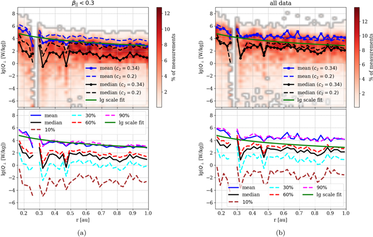
Figure 2. Perpendicular solar wind heating rate due to SH in low-β plasma streams, calculated using Equation (2) in panel (a) and using the general expression given in Equation (6) in panel (b), throughout two PSP encounters (for r ≤ 0.25 au) and the entire Helios 1 and 2 missions (for r ≥ 0.29 au) using c2 = 0.34. Results that include high-β streams (Equation (6)) are significantly higher for both mean and median. The radial trend Q⊥ ∼ r−2.5, fitted from Helios observations by MKB19, is shown by the green solid line, matching well with the results on panel (b), while in panel (a), we observe slightly stronger radial trend closer to the Sun. Results using c2 = 0.2 (dashed lines) follow similar trends but with notably higher amplitudes. Data shown in the upper panels are column-normalized inside each radial bin, with results inside each column being uniformly binned in the logarithmic space. Lower panels show percentiles of the Q⊥ distribution, which is highly skewed toward higher values, even in logarithmic space. Only ∼10–15% of measured values are above average, and these contribute the most to the total SH in the solar wind.
Download figure:
Standard image High-resolution imageIn order to compare the measured Q⊥ values with the total perpendicular heating of the solar wind protons, we estimate the total empirical heating rate Q⊥emp using Equation (9). As explained in Section 2, all results are organized in bins divided by speed and radial distance and shown in different colors on Figure 3. Weighted averages that take into account the number of measurements in each of the velocity bins, as well as their uncertainties, are shown by black dots. These results are compared with SH rates calculated using Equations (2) and (6), marked by red and blue dots (PSP) and squares (Helios), respectively. The black dashed lines represent a simple model used by Bourouaine & Chandran (2013), based on evaluating Equation (9) at r = 0.29 au and extrapolating the result using radial trends of B, vsw, and vt⊥ measured by Helios, while the dashed red line shows the two-fluid model developed by Chandran et al. (2011), which is expected to be increasingly accurate closer to the Alfvén point. Predictions based on Helios measurements for fast and slow solar wind, filtered as vsw < 400 km s−1 (Hellinger et al. 2013) and vsw > 600 km s−1 (Hellinger et al. 2011), are shown by blue and green dashed–dotted lines. For all of the four data sets shown, we note that the SH rates are comparable with the total estimated heating rates at radial distances covered by PSP results, while for r > 0.3 au covered by Helios measurements, SH rates are lower than total heating rates, both measured and predicted by models, except for the results of Hellinger et al. (2013), which are relevant to slow wind only.

Figure 3. Estimated turbulent heating rates derived from MHD plasma parameters, following Bourouaine & Chandran (2013) for PSP encounters 1 and 2, inbound and outbound. Black dots represent weighted averages of the total empirical perpendicular heating rates, while colored stars show the same results binned into slow, intermediate, and fast solar winds. Estimated values of SH for low-β plasma (filled red dots) and for all β values (filled blue dots) are of the same order of magnitude as the total estimated heating rate for PSP measurements (except during E1 inbound phase), while that is not the case for Helios measurements (squares). Both measurement sets are also comparable to theoretical models (Chandran et al. 2011; Bourouaine & Chandran 2013). SH rate values measured by PSP are consistently enhanced for c2 = 0.2 (hollow circles).
Download figure:
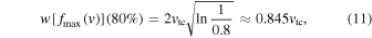
Standard image High-resolution imageThat the radial trend of total heating is significantly stronger in the fast solar wind is well-known, being Q ∼ r−1.8 (Hellinger et al. 2011), compared to Q ∼ r−1.2 for the slow wind (Hellinger et al. 2013), leading to the correlation of the solar wind bulk velocity and temperature. This difference is even more visible for SH results, where MKB19 found Q⊥ ∼ r−3.1 for the fast wind in Helios results. Figure 4(a) displays dependence of the low-β Q⊥ on the solar wind bulk velocity, where Q⊥ increases for two orders of magnitude as vsw changes from 280 to 750 km s−1. This trend is a direct consequence of a linear δ−vsw correlation in Figure 4(b), which implies that this significant increase in Q⊥ originates from the intensity of turbulent fluctuations.
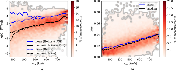
Figure 4. Values of the perpendicular SH rate Q⊥ (a) and δ (b) are plotted against the solar wind bulk velocity (only low-β plasma measured by both Helios and PSP is considered). The general logarithmic increase of Q⊥ with vsw is notable, with values being significantly more spread for lower solar wind speeds. As influence of PSP measurements is visible only for vsw < 600 km s−1, mean and median values from Helios results only are plotted separately as dashed lines to demonstrate the trend similar to the one shown on panel (b). Data in all of the panels shown are column-normalized inside each velocity bin.
Download figure:
Standard image High-resolution imageFinally, we perform a comparison of the SH values with the proton VDF shape. Diffusion calculations of the SH-dominated plasma by Klein & Chandran (2016) showed that thermal protons moving slowly in the perpendicular direction are more significantly affected by SH compared to protons with larger velocities in the perpendicular tail of the distribution. This behavior implies that those protons with the lowest perpendicular velocities are the ones gaining the largest amount of energy. The described effect is dominant only until particles reach velocities of the order of vt, where their orbits become smoother (less stochastic) and SH from ion-scale fluctuations becomes less effective, resulting in a flattop-shaped reduced perpendicular distribution. In panel (a) of Figure 5, we show example of a flattop-shaped reduced VDF measured in the fast solar wind (blue dotted solid line) perpendicular to the magnetic field. As the routine algorithm used by the instrument team assumes a Maxwellian core, the quality of the fit (blue dashed line) is poor and the obtained core temperatures might be overestimated; see Figure 3 of Klein & Chandran (2016). We see that the flattop distribution corresponds to significantly stronger turbulent fluctuations compared to intervals with Maxwellian-like VDF measured in the slow wind (orange lines), with δ and parameters that are twice as large. The Q⊥ calculated using Equation (2) (both measurements are from low-β streams and the same radial distance) is three orders of magnitude larger for the case of a flattop-shaped core VDF than for a Maxwellian one.

Figure 5. (a) Example of normalized measured reduced VDFs in the plasma frame, both perpendicular to the magnetic field, at radial distance of r = 43.86R⊙ (0.205 au) on 2018 November 2, 16:05 (orange) and 2018 November 9, 15:10 (blue). Maxwellian distributions with core temperatures provided by the instrument team are given by dashed lines. Panel (b) shows mean values of the VDF width at 80% of the maximum value divided in 20 θ angle bins (of 9° each), normalized to the core temperature vtc. The mean VDF width is notably increasing with the solar wind speed for θ ∼ 90°, which indicates the presence of flattop distributions. Dashed lines map to the right-hand ordinate axis of panel (b) show the number of VDFs sampled per angle and velocity bin, demonstrating that PSP has dominantly observed the slow solar wind, while statistics for the fast wind in the radial and antiradial directions are poor.
Download figure:
Standard image High-resolution image
In the same work, Klein & Chandran (2016) fitted their flattop VDFs with a modified Moyal distribution (Moyal 1955), which is characterized by decreased values of excess kurtosis κ ≈ −0.8 compared to the Maxwellian value of κ = 0. However, this metric is only useful for analytic distributions spanning the entire velocity space. Even though a modified kurtosis can be derived for distributions that cover a finite but constant velocity range, our measured VDFs cover velocity ranges that change from distribution to distribution, depending on which of the detector velocity (voltage) channels are not polluted by the instrument noise. These range changes affect the calculated kurtosis, confusing the physical interpretation of the values. Therefore, we track the systematic appearance of flattops by establishing a more direct criterion. We calculate the full width of the VDF at 80% of its maximum height. This value is large enough to avoid influence from the proton beam or α particle populations. The width is normalized by the thermal velocity of the fitted core distribution vtc, both to avoid the effects of the vsw ∼ vt correlation and to enable comparison with an equivalent Maxwellian distribution fmax(v), which has width w at 80% of intensity
where ln is the natural logarithm. Results are shown on Figure 5(b), where the solar wind is separated into three bins: slow, intermediate, and fast. Slow wind results are below the referenced Maxwellian value, which is the effect of a finite measurement resolution combined with the generally colder, slower wind.21
Importantly, the normalized widths of VDFs systematically increase with solar wind speed, which implies that they also increase with measured values of Q⊥ (Figure 4(a)). This effect is visible when a reduced VDF is measured in the direction perpendicular to  for vsw > 550 km s−1, as expected from theoretical predictions (Klein & Chandran 2016). Increased widths that appear for low values of θ in the slow wind originate from measurements where the VDF maximum appears just next to the noisy low-energy channels. However, radial and antiradial orientation bins are not covered with sufficiently strong statistics (green dashed line on panel (b)), so measurements from future PSP encounters will be required to examine these in more detail.
4. Discussion
The results shown in Section 3 provide the first insight into the solar wind perpendicular heating rate measurements for radial distances in the range 0.16–0.25 au. As such, we can test previously measured trends from larger distances and theoretical predictions.
It is particularly worth emphasizing that radial trends found in MKB19, which predict SH to be a significant fraction of the total solar wind heating closer to the Sun, are sustained at the radial distances covered by the first two PSP encounters. MKB19 estimate SH rate to be relatively insignificant at 1 au (with model parameters obtained also being in accordance with results of Vech et al. (2017)), but having strong radial scaling as Q⊥ ∼ r−2.5, compared to the total heating rate scaling of Q⊥emp ∼ r−2.1. This difference is even more significant in the fast solar wind, being Q⊥ ∼ r−3.1 against Q⊥emp ∼ r−1.8, measured by Hellinger et al. (2011). Analyzing results shown on Figure 3, we can compare the estimated total solar wind heating rates with the estimated SH rates. Total heating rate is shown by black dots, while the results obtained by the same method for larger radial distances are given by a dashed line provided by Bourouaine & Chandran (2013). These values are either comparable to or smaller than the estimated SH rates (red and blue circles) for r ≲ 0.2 au, with even low-β measurements becoming comparable to the empirical heating rates estimated using Equation (9).22 Of course, SH being higher than total heating rate is an unphysical result, but is still within range of relatively large measurement uncertainties, which are approximately one order of magnitude for both sets of values. On the other hand, SH rates estimated from Helios measurements are either systematically lower than or comparable to the observational results given by the dashed black line. Considering these results and findings from MKB19 and Vech et al. (2017), we conclude that SH is playing an increasingly important role in the solar wind heating as the radial distance decreases, and is possibly becoming a dominant heating mechanism in the near-Sun solar wind.
For further testing of this statement, we were able to obtain measurements of flattop-shaped distributions, as shown in Figure 5. This result is in accordance with predictions of the model that assumes dominant SH (Klein & Chandran 2016). Figure 5(a) gives an example of a flattop distribution at r = 0.205 au during the encounter 1 outbound phase, with an SH rate that contains a significant fraction of total heating predicted both by models and the total heating calculation (Figure 3, upper right). Even though the statistics of fast wind measurements are poor, we found that this VDF shape in the direction perpendicular to  is commonly measured in the fast wind, as shown in Figure 5, panel (b). However, although our results suggest that the SH rate is similar to the estimate of the total heating in the fast wind and visual inspection of the measured VDF shows the flattop shape, averaged values of normalized VDFs in the fast wind shown on Figure 5(b) imply that a modified Moyal distribution is not fully developed. The observed averaged distributions have width at 80% of maximum of approximately w ≈ vt, while the Moyal, as predicted by Klein & Chandran (2016), has a notably larger value of the same parameter at w ≈ 1.3vt. Due to limitations of the data set, at this point is not possible to distinguish if this discrepancy between theory and observations is caused by mechanisms other than SH notably participating in the proton diffusion in velocity space (and consequently, heating of the solar wind) or by SH being the dominant heating mechanism, but the modified Moyal VDF shape is not sustainable in realistic solar wind conditions. A recent argument in Isenberg et al. (2019) suggests that extreme flattop-shaped distributions can be suppressed by a quasi-linear ion-cyclotron anisotropy instability for large temperature anisotropy in very low-β plasma. In the measured streams, we have
  on more than 90% of the intervals (J. Huang & SWEAP 2019, in preparation), so this effect is not expected to dominate at the PSP distances, but rather to be a competing process with the perpendicular particle diffusion described by Klein & Chandran (2016), with importance depending on multiple parameters. A possible interpretation of the observed shape is that the ion-cyclotron instability could be important close to the Sun and we observe a more Maxwellian-like VDF shape after strong instabilities have been saturated.
An important property of the results shown on Figure 2 is that Q⊥ varies over 10 orders of magnitude, with only ∼10–15% of values being above average, and there is a difference of two orders of magnitude between mean and median. This is seen in both Helios and PSP measurements. These features have been discussed in detail in MKB19, where it was argued that lg(Q⊥) and δB follow a Gaussian distribution with an addition of a broad low-energy tail. This tail is associated with the pristine, low-turbulent amplitude solar wind and negligibly contributes to mean heating values. Also, due to strong vsw − δ correlation visible on Figure 4(b), the spread in Q⊥ is much lower if the slow and fast winds are treated independently. Finally, effects of highly intermittent turbulence are not taken into account in this work. Strong intermittency can significantly increase the SH rate, according to recent theoretical results (Mallet et al. 2019). Case studies of intermittent intervals are a separate topic for future work.
Along with discussing these results, we need to be aware of all of the limitations of both methods and measurements used. The PSP high-resolution data from encounters 1 and 2 cover only two encounter periods of 11 days, separated by a five-month span between the two closest approaches. Therefore, we do not expect a large, statistically complete set of results, but only a "randomly picked" sample of solar wind plasma at 0.16–0.25 au, almost 90% of which is from the slow solar wind. In contrast, SH (and solar wind heating in general) is expected to be more effective in the fast solar wind, where our measurements are severely lacking. Measurements from a few streams lasting several hours each at r ∼ 0.2 au during the E1 outbound phase are the rare exception. These fast wind results correspond to the maxima at Figure 3 (upper right) for both stochastic and total heating, as well as to the illustrative example on Figure 5(a). An analysis that grants wider insight into SH behavior in the slow and fast streams separately, analogous to the one performed for Helios data in MKB19, will be possible once the data set is enlarged during the following encounters. In investigating intervals near and in Alfvenic "spikes" (Horbury et al. 2020), increases in both fluctuation amplitudes and Poynting flux were observed near the spike boundaries (Kasper et al. 2019; Horbury et al. 2020). This relatively short (up to tens of seconds) timescale boundary effect is not expected to be important for the results presented here, as we use 10 minute–averaged measurements, but properties of SH in different scale structures are a separate topic for future work. This kind of case study is, with current instrumentation, possible only for PSP and at 1 au, due to the lower quality and resolution of Helios measurements at intermediate radial distances.
Combined with the uncertainties in measurements, it is important to note that the SH calculation method described in Section 2 can only provide order-of-magnitude estimates of Q⊥, due to selected values of the model constants c1, c2, σ1, and σ2. In this work, we use values provided by test particle simulations for randomly phased Alfvén waves (Chandran et al. 2010; Hoppock et al. 2018). Values of c1 and c2 were also examined by Xia et al. (2013) in test-particle simulations, but with the test particles interacting with RMHD turbulence rather than randomly phased waves, significantly lower values of c2 ∼ 0.2 were found. This value is used as an alternative in our model in Figures 2 and 3, demonstrating that estimated low-β SH rates are increased by more than an order of magnitude. No other estimates of σ1 and σ2 are available beyond those provided by Hoppock et al. (2018). Detailed discussion on constants is provided in MKB19. Finally, it is important to note that the σ factor, which connects magnetic and velocity fluctuations, assumes Alfvénic turbulence. If the turbulence is not purely Alfvénic, this value could vary, which would produce an effect similar to changing c2 or σ2—a notable variation in Q⊥ for high-β plasma. Finally, we conclude that all the factors described here enable us to determine only the order of magnitude of the SH rate, in a fashion similar to the Helios data analysis in MKB19. On the other hand, simulation results (Chandran et al. 2010; Xia et al. 2013) show that the values of model constants, although unknown, are not very sensitive to plasma parameters, and are therefore still usable in determination of the radial trends related to SH, which was discussed above.
In the encounters to come, we will aim to further test these results with a larger sample of fast wind measurements at different radial distances. Once a more robust data set becomes available, a case study of these particular intervals, relying on the assumption that they are determined by SH as the only solar wind proton perpendicular heating mechanism, will provide useful constraints on the model constants and significantly reduce uncertainties of the SH rate amplitudes.
We expect an increased level of turbulence below the Alfvén point, predicted by theoretical models (Matthaeus et al. 1999) and MHD simulations (Perez & Chandran 2013; Chhiber et al. 2018; Chandran & Perez 2019), to effectively drive SH. Recent results (Kasper & Klein 2019) indicate that the region of preferential minor ion heating (Kasper et al. 2017) terminates at the Alfvén surface. Whether SH is the preferential heating mechanism operating in this region will be determined by future PSP measurements within this region. With the data from the first two encounters, we argue that SH tends toward being the dominant solar wind proton heating mechanism as PSP approaches the Alfvén point, especially in the fast solar wind streams. This is consistent with both Helios analysis and both approaches presented in this work—determination of SH rate using theoretical formalism (Chandran et al. 2010; Hoppock et al. 2018) and analysis of VDF shapes according to the predictions made by Klein & Chandran (2016), as well as comparison of these results with the total heating rate estimate from PSP data and theoretical models (Chandran et al. 2011; Bourouaine & Chandran 2013).
The SWEAP Investigation and this publication are supported by the PSP mission under NASA contract NNN06AA01C. The FIELDS experiment was developed and is operated under NASA contract NNN06AA01C. M.M.M. and K.G.K. were financially supported by NASA grant 80NSSC19K1390. B.D.G.C. is partially supported by NASA grants NNX17AI18G and 80NSSC19K0829. C. H. K. C. is supported by STFC Ernest Rutherford Fellowship ST/N003748/2.
Footnotes
- 16
AWs were also observed by remote infrared measurements in the solar corona (Tomczyk et al. 2007).
- 17
An SPC operation mode that allows the study of high-cadence velocity fluctuations, called the Flux Angle Mode, was active during a few limited time windows within the first two encounters. This mode, which samples a single energy channel very rapidly (Vech et al. 2020), could potentially be used for verification of Equation (5) in future work, as well as for the direct evaluation of Q⊥.
- 18
The expression for the convective gyrofrequency in MKB contains a typographical error; a factor of 2π is missing from the denominator. Also, Equation (8) of MKB19 should be identical to Equation (3), while that version has the factor fp inside the exponential factor in the integral boundaries. Neither of these typographical errors affect the contents presented in that article.
- 19
Outside of encounter 1, the Fields magnetometer resolution drops to Δt ≈ 0.43s, while outside of encounter 2 we have Δt ≈ 0.1. This value sets the Nyquist frequency just below 5 Hz and could be, with some improvement of the method (i.e., more sophisticated treatment of the spectral break), used in our work. However, magnetometer data are missing for significant time periods, and the SPC measurements for those periods have resolution comparable to the time window used (10 minutes) or are flagged by the instrument team as unreliable, so a potential upgrade of our processing methods in order to cover this very limited set of measurements is left for future projects.
- 20
- 21
As the SWEAP instrument is designed for maximum efficiency at the PSP closest perihelion (r ∼ 10R⊙), measurements during encounters 1 and 2 were collected at the "outer limits" of SPC's characteristics, while future observations are expected to have significant improvements in both signal-to-noise ratio and VDF resolution around the maximum (Kasper et al. 2016; Case et al. 2020).
- 22
The solar wind during the inbound phase of encounter 1 has been determined to be corotating with a small coronal hole (Bale et al. 2019; Badman et al. 2020), and it has been reported (Bale et al. 2019) that the turbulent fluctuations are very low in this period, which causes the measured SH values to be significantly lower then those obtained from MHD models, as shown on Figure 3 (upper left).