


Abstract
The parameter distribution of binaries is a fundamental knowledge of the stellar systems. A statistical study on the binary stars is carried out based on the LAMOST spectral and Kepler photometric database. We presented a catalog of 1320 binary stars with plentiful parameters, including period, binary subtype, atmosphere parameters (Teff, [Fe/H], and  ), and the physical properties, such as mass, radius, and age, for the primary component stars. Based on this catalog, the unbiased distribution, rather than the observed distribution, was obtained after the correction of selection biases by the Monte Carlo method considering comprehensive affecting factors. For the first time, the orbital eccentricity distribution of the detached binaries is presented. The distribution differences between the three subtypes of binaries (detached, semidetached, and contact) are demonstrated, which can be explained by the generally accepted evolutional scenarios. Many characteristics of the binary stars, such as huge mass transfer on semidetached binaries, period cutoff on contact binaries, period–temperature relationship of contact binaries, and the evolved binaries, are reviewed by the new database. This work supports a common evolutionary scenario for all subtypes of binary stars.
Export citation and abstract BibTeX RIS
1. Introduction
Binary stars are probably the most familiar variable stars to astronomers, due to their enormous number and the irreplaceable features for providing model-free stellar basic properties (Gorynya & Tokovinin 2014; Wilson & Van Hamme 2014; Gaulme et al. 2016). The first variable object documented by humankind was a binary system5 more than 3000 yr ago (Jetsu et al. 2013), and binaries hold the most significant number of variables observed so far, accounting for about a quarter of all variables (Watson et al. 2006, 2015).
Thanks to the large-scale ongoing and upcoming surveys such as LAMOST, Kepler, Gaia, TESS, LSST, data of unprecedented quality, volume, and dimensionality allow us to study all kinds of celestial objects, including binaries, in a thorough manner. The observations in the past were fragmentary, disunited, and variously biased, partly leading to knowledge on a class of diversified stars and their uncertainty. However, now the current surveys have dramatically improved the situation as never before. This work is an effort on the distribution of binary parameters based on two significant projects, LAMOST (Large Sky Area Multi-Object Fiber Spectroscopic Telescope) and Kepler.
The field of eclipsing binary stars benefited from LAMOST and Kepler a lot. More than 2500 eclipsing binaries (LaCourse et al. 2015; Kirk et al. 2016), 10 transiting circumbinary planets (Welsh et al. 2015; Feinstein et al. 2019), and 10 eclipsing multiple stellar systems (Zhang et al. 2018) have been discovered by the Kepler spacecraft photometrically confidently. More than 200 Kepler binary systems with third bodies were revealed by the light-travel time effect or dynamical delays based on the extraordinary evidence of eclipse time variation (ETV; Rappaport et al. 2013; Borkovits et al. 2016, 2019). Kepler had greatly contributed to the field of pulsating stars, and nearly all the recent studies on pulsating stars in binary systems rely on the Kepler data (Lee & Park 2018; Murphy 2018; Johnston et al. 2019). The binary fraction in our Galaxy was investigated depending on the huge LAMOST spectral database (Gao et al. 2014, 2017; Yuan et al. 2015; Tian et al. 2018). More than 250,000 new variable candidates are discovered from the LAMOST database (Qian et al. 2019).
The purpose of this work is to take advantage of the outstanding photometric data from Kepler and the vast amount of spectral data from LAMOST and to study a large number of binary samples statistically after the correction of selection biases. A catalog of 1320 binary stars is obtained, based on which a batch of relationships between various parameters is presented and investigated. After careful correction on the selection bias, we provide an unbiased distribution on binary stars, consisting of both eclipsing and noneclipsing binaries. Based on the binary distributions, the connection between different binary subtypes and the evolutional scenario was discussed. At last, the distribution of the parameters delivers some interesting clues on the evolution of the binary stars.
2. Kepler and LAMOST Data
The Kepler spacecraft brought fantastic photometry data owing to its two distinct features. The first one is that Kepler focused on a fixed sky region of 115 deg2 for 3.5 yr in the way of generally uninterrupted exposure.6 Thanks to this point, for the first time we have detected many long-period binaries (>1 yr) that undoubtedly were never achieved before. The cumulative observation time of the Kepler spacecraft (more than 1000 days) is probably long enough to cover the orbital periods of the vast majority of binaries, which will be illustrated in the following section of the period distribution.
The second feature of Kepler is the unprecedented photometric precision of 20 parts per million (ppm), reaching the desired limit of light variation by eclipsing binaries. The actual performance of Kepler is even more impressive for the finding of some eclipsing binaries with only 0.0002 mag amplitude of variation (e.g., KIC 11197853). Not surprisingly, Kepler is originally devoted to discovering Earth-size planets through the tiny light reduction caused by the planets transiting their host stars. Kepler has found many noneclipsing binaries with little light variations by the light reflection effect and deformation of the star shape. Such high precision makes almost all eclipsing binaries detectable, including the marginal eclipsing binaries as long as the object was bright enough.
The Kepler eclipsing binary stars were cataloged thoroughly (Prša et al. 2011; Slawson et al. 2011; Matijevič et al. 2012; Conroy et al. 2014a, 2014b; LaCourse et al. 2015; Kirk et al. 2016), containing parameters such as orbital periods, the morphology of light curves, and phase positions of secondary minimum on which this work depends.
LAMOST, a large ground-based spectral survey telescope, carried out dense spectral observations on the sky within −10° to 60° of northern latitude and had already acquired more than 8 million stellar spectra. Its observation area nicely covered the fixed field of view of Kepler.
The LAMOST data we used come from DR4 (the observation duration is from 2011 October 24 to 2016 June 2), which is freely available all over the world. Given that our targets are all binary stars, the atmosphere parameters were remeasured by taking into account the rapid rotation of stars in the binary systems (as opposed to using the official parameters provided by the authorities). Besides, the measurable range of temperatures was expanded to derive a binary parameter space as large as possible. The actual temperature range is from 4131 to 36,000 K, which is reasonably large for binary stars. This effort aims to reduce the statistical bias caused by the inadequate parameter space, and it is believed that this broad range does not leave out many binaries that can destroy the statistical results.
3. The Physical Properties Derived from LAMOST and Kepler Observations
3.1. Parameters from Kepler
Based on the light curve from Kepler, the binary subtypes (contact, semidetached, and detached), precise orbital periods, and the positions, depths, and widths of eclipses can be acquired directly, which is the basis of this work. If the modeling analysis of the binary light curve was carried out, a series of relative parameters, such as mass ratio, luminosity ratio, and radius ratio, can be obtained. Despite this, the modeling analysis was not performed in this paper owing to the enormous amount of computer work with multifarious manual adjustments, which deserves to be independent work.
3.2. Parameters from LAMOST
LAMOST provided the spectra of binaries, from which the atmosphere parameters, i.e., Teff, [Fe/H],  , and Vr, were measured with ULySS (Universite de Lyon Spectroscopic analysis Software; Koleva et al. 2009; Wu et al. 2011b, 2011a, 2014). The measurement adopted the single-star model, but our targets are binary stars. So the problem is, which component star do the parameters pertain to—the primary star, the secondary star, or none of them?
Technically, the measured parameters do not pertain to any of the component stars, but only reflect an average value for the whole binary system. However, such an average value is no use to our study, so we have to make an approximation. It is assumed that the atmosphere parameters measured from the spectra approximately represent the brighter component star that dominates the light of the whole system. The reason is that the light dominant component star mainly contributes the light received by the telescope from the binary system, and therefore the spectra observed should primarily reflect the brighter component star. If there is no dominant star in a binary system (for instance, two components are comparable in luminosity to each other), the two components with comparable luminosities probably have similar atmospheres. Thus, statistically, the above approximation holds.
To verify the approximation quantitatively, we will examine the data in two different ways. The first way is that the spectra of two certainly single stars with well-determined parameters were merged to fabricate one binary spectrum. The atmosphere parameters of this artificial binary spectrum were measured and then compared to those of the brighter single star. The test carried out by C. Liu (2017, private communication) based on MILES spectral library (Medium resolution INT Library of Empirical Spectra, Sánchez-Blázquez et al. 2006; Vazdekis et al. 2010) shows that the difference between the measured temperatures and the brighter single stars' temperatures are almost within 200 K, no matter what the mass ratio of the two single stars is.
The second way is to compare our temperatures to the work of Armstrong et al. (2014), who obtained the temperatures of the two component stars by photometry data from HES, KIS, and the Two Micron All Sky Survey. The comparison shows that the temperatures derived from LAMOST spectra match with those of the primary stars with no visible overall deviation despite the large dispersions. Moreover, for the comparison with the temperatures of the secondary stars, the LAMOST temperatures are hotter in general; see Figure 1. The large dispersions are probably chiefly due to the errors of Armstrong et al. (2014), which are 370 K in primary temperature and 620 K in secondary temperature. Since no systematic deviation was found between the LAMOST temperatures and the primary temperatures, the approximation above is generally valid.

Figure 1. Temperature comparison of the binary stars between LAMOST and Armstrong et al. (2014) for the primary stars (left) and the secondary stars (right). The red lines are the isothermal lines. The colors of the dots indicate the density of the dots, from dense (yellow) to sparse (blue).
Download figure:
Standard image High-resolution imageThe  is not tested as the temperature. However, considering that the typical error of
  is large (∼0.2), the measured value should be consistent with the primary stars within the error range. For the metallicity, the two components in a binary system are likely the same, if two stars are thought to originate from the same cloud. Therefore, the measured value should not be much different from that metallicity.
Not all kinds of spectra can be measured for the atmosphere parameters. Usually, only the stars of spectral type A, F, G, and K can be provided with atmosphere parameters, but stars of O, B, earlier A, or late K and M type cannot. This is because the reliable templates for too hot or too cold stars are not adequate for the pipeline. Moreover, the spectra of low-temperature stars (≲3000 K) are far from clear in theory, so no valid theoretical template is available.
The temperature range of the binary samples in this work is 4131–36,000 K, which excludes the M, late K, and O-type stars. Although the measured temperatures from the LAMOST spectra can be as low as 3300 K, the atmosphere parameters of the cool stars are perhaps not reliable because they are hard to fit into a theoretical model. The ranges of  and [Fe/H] of the binary sample are 1.844–4.812 dex and −2.473 to 0.784 dex, although the pipeline can reach a broader range of −0.189 to 4.9 in
  and −2.5 to 0.99 in [Fe/H], which cover nearly all kinds of stars.
Although the photometric observations of Kepler are not limited by the targets' temperature, the atmospheric parameters derived from the LAMOST spectra are limited by the temperature. Hence, the final binary samples for statistics are still confined within a temperature range.
3.3. Stellar Properties Estimated from the Atmosphere Parameters of LAMOST
If the atmosphere parameters derived from binary spectra can represent the primary stars as discussed above, the physical properties of the primary stars can be estimated from the atmosphere parameters by matching with stellar isochrones. The isochrone database we used is PARSEC (PAdova and TRieste Stellar Evolution Code; Bressan et al. 2012; Chen et al. 2014, 2015; Tang et al. 2014), along with the lognormal form initial mass function by Chabrier (2001). The Teff, [Fe/H], and  deduced from LAMOST spectra were utilized to determine the primary stars' physical properties, including mass, radius, age, and rough evolutionary stage.
Figure 2 is an illustration for the estimation of the physical properties of KIC 6579806 from the three atmosphere parameters. The red symbol stands for the position of the primary component of the binary target, and the black symbols are the stars selected from PARSEC for which atmosphere parameters are close to our target (red symbol). The ranges of the black symbols are just equal to the errors of the binary target. The physical properties (such as mass, radius, and age) of the closest black symbol to the red symbol are assigned to the target binary, and the ranges of all the black symbol parameters are regarded as the errors of the physical properties.
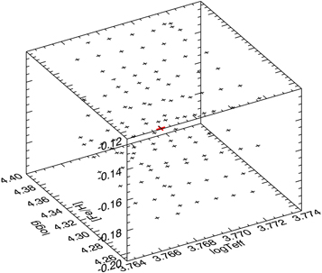
Figure 2. Illustration for the estimation of the physical properties of KIC 6579806 from the three atmosphere parameters.
Download figure:
Standard image High-resolution imageThere is a problem when it comes to the closest black symbol: how do we determine the distance since the three atmosphere parameters have different dimensions? Here it is defined that the errors of the three atmosphere parameters are equal to each other in the sense of "distance." The atmosphere parameter errors of KIC 6579806, for example, are 144 K in Teff, 0.267 index in  , and 0.165 index in [Fe/H]. When calculating the distance, the definition is that 144 K (Teff) equals 0.267 index (
 ) and also equals 0.165 index ([Fe/H]). Thus, the distances between every black symbol and the red symbol in Figure 2 can be calculated. It is conceivable that the definitions are different from one target to another owing to their various errors.
If we do not use the method of the closest point described above, an interpolation method is needed. Based on the relationship between any parameter and the distance calculated above, the target parameters can be interpolated at a distance equal to zero. The outcomes from this interpolation method are very close to those from the most adjacent point compared to their errors. Because the interpolation at a distance zero is the extrapolation mathematically, ridiculous results may thus arise. For the sake of safety, all the physical properties of the primary stars are taken from the nearest point.
4. The Correction on Selection Bias
If we want to make an unbiased distribution on binary parameters, the correction on selection bias is unavoidable. According to the collection by the International Variable Star IndeX (VSX; Watson et al. 2006; Gonzalez 2015), more than 100,000 eclipsing binaries have been observed and studied, which is a high number. However, a reliable distribution is still unclear because the sources of these binaries are diverse and jumbled, together with various observational methods, purposes, and instrumental limitations, making the correction on the selection bias very difficult if not impossible. Accordingly, the actual distribution is not a natural consequence of the increasing quantity of samples.
This situation was greatly improved by the presence of the Kepler mission because of its two outstanding features. The first one is the unprecedented photometric precision of 20 ppm, making very tiny eclipsing light variation detectable. The Kepler spacecraft had found many noneclipsing binaries. The second feature is the 3.5 yr photometric monitoring on a fixed field of view covering 115 deg2, which enables coverage on a rather long orbital period scope. Kepler can safely cover the eclipsing binaries with orbital periods less than 1 yr, and a considerable proportion for periods less than 3 yr. These two features had never been achieved before, and hence it can be said that the Kepler mission shed new light on the research field of binary stars.
If we only have the photometric data from Kepler, the understanding of the binaries is very limited because the light curve cannot provide absolute physical properties. Fortunately, the spectroscopy survey by LAMOST compensates this shortage very well. The LAMOST spectroscopically observed more than 1 million stars in the northern sky that nicely covered the field of view of Kepler. The LAMOST telescope carried out extra intensive observations on Kepler targets and accordingly covered about half of the Kepler binaries.
Because the source of these binary samples is unified and the way of discovering them is quite thorough, in addition to their plentiful parameters, the correction on the selection bias is feasible based on only a few reasonable hypotheses. The Monte Carlo method was applied to correct the selection bias. Because Kepler had already swept out nearly all the eclipsing binaries in the Kepler database, the correction on the selection bias is equivalent to calculating how many noneclipsing binaries there should be.
It is worth mentioning that the binaries discovered by Kepler contained noneclipsing binaries, but only the eclipsing binaries are used to correct the selection bias for the real distribution of the binaries. The noneclipsing binaries are not taken into account for the correction because the detection on noneclipsing binaries is far from complete (although many of them were detected). A premise of the correction is the acceptable completeness and exclusiveness in some aspects. In this work, it means that all the observed eclipsing binaries were discovered successfully, and only the eclipsing binaries were used for the correction.
4.1. Correction on the Eclipse
Although many binary parameters are already obtained, they are not enough to determine whether the eclipses occur or not. Only three of them are directly related to the eclipses, which are period, mass, and radius of the primary star. However, five more parameters are required, including the inclination, mass, and radius of the secondary star; the orbital eccentricity; and the longitude of periastron. For each binary sample, we need to calculate the probability of the eclipses occurring.
If the calculated probability is 10% for a binary sample, it means that only 10% of the binaries with the same known parameters as the binary sample are eclipsing binaries, while the other 90% are not eclipsing binaries and so cannot be discovered photometrically. In other words, if one binary sample was discovered photometrically, there should be nine other noneclipsing and undiscovered binaries with the same known parameters. Therefore, this binary sample should be counted as 1/10% = 10 in statistics in order to include all the binaries. It can be predicted that the probability for long-period detached binaries is much lower than that for contact binaries.
For the unknown parameters that are related to eclipses, their distributions need to be assumed or calculated. For each binary sample, all of its unknown parameters will be generated to be many sets of artificial values according to the distributions. Each set of parameters constitutes an artificial binary star with the complete parameters, by which we can judge whether the eclipse occurs. Thus, the number of artificial eclipsing binaries can be counted among a large number of the generated artificial binaries. The proportion of the artificial eclipsing binaries is used to correct the selection bias for every binary sample.
It is unrealistic and unreliable to assume the distributions for all five unknown parameters. Two known parameters, the metallicity and the age of the binary system, can help us to solve the problem. Accordingly, only the distributions of three parameters need to be assumed, and then all the unknown parameters can be calculated. The three parameters are the orbital inclination, longitude of periastron, and mass ratio. We will describe the assumption of the distributions and the calculation for all the unknown parameters in the following.
The first and the most critical parameter is the orbital inclination, which is assumed to be evenly distributed in the three-dimensional direction. This is a fairly natural assumption, and there is no evidence of the tendency in any particular direction. If we want to test this assumption, much more extensive and thorough observations of all binaries should be carried out, including those with nearly zero degrees of inclination. This work is not as impossible as it seems, because for contact binaries Kepler can detect almost all of them even with pretty small inclination.
With the help of the binary light-curve analysis, all contact binaries' inclination can be worked out. So the comprehensive and unbiased inclination distribution from the contact binaries is obtained, which could represent all the binaries because the inclination does not change with the binary subtype. This work, although feasible, is enormous. So the assumption of spatial isotropy on inclination is adopted in this paper.
The mass and radius of the secondary star also affect the eclipse of the binary system. In order to calculate the secondary mass, a power-law mass ratio distribution f(q) ∝ q0.3 is adopted as in Tian et al. (2018) and Raghavan et al. (2010). The distribution is zero at mass ratio equals zero and monotonically increases to mass ratio equals unity. Although the mass ratio distribution of binary stars is very crucial, a generally accepted conclusion is still pending. Based on the mass ratio and the primary mass, the secondary mass can be calculated.
For the radii of the secondary stars, the method of isochrone interpolation was used as in Section 3.3, where the physical properties of the primary stars were estimated from the atmosphere parameters. Now, the difference is that the input parameters are mass, metallicity, and age rather than the atmosphere parameters. Here it is assumed that the two component stars in a binary system share the same metallicity and age. If the two component stars originated from the same cloud, this assumption is quite reasonable. Since the metallicity and age of the primary stars are already known, so are those of the secondary stars. To gain a more suitable outcome, a limitation is selected that the luminosity of the secondary star is lower than that of the primary star. This limitation accords with our definition of the primary star above. By all the above, the radii of the secondary stars can be calculated.
The orbital eccentricity and the longitude of periastron are another two parameters affecting the eclipses. The longitude of periastron was assumed to be evenly distributed between 0 and 2π, which is again a very natural and even obvious assumption. By this point, the phase position of the secondary minimum is very useful. Combined with the phase position and the longitude of periastron, the orbital eccentricity can be calculated. Thus, the assumption on the distribution of the eccentricity is no longer necessary. The phase position can provide us a quantity of  (Kopal 1959, page 385), so the eccentricity e can be worked out if the longitude of periastron ω is given. Actually, the eccentricity distribution is obtained as a result of this paper.
Up to now, all the unknown parameters related to eclipses were assumed with distribution or were calculated. Among the three parameters with the assumed distributions, i.e., the inclination, longitudes of periastron, and mass ratio, the assumptions of the first two parameters are very natural. Nevertheless, the distribution of mass ratio brings large uncertainty, which should be improved in the future.
To calculate the probability of the eclipses occurring, 10,000 sets of inclinations, the longitude of periastron and mass ratios were randomly generated according to the assumed distribution. These 10,000 sets of parameters were assigned to each binary target to create 10,000 artificial binaries, and then it can be calculated how many of them will and will not eclipse. The proportion of the eclipse cases is the probability used to correct the selection bias caused by eclipses.
Tests indicate that 10,000 is numerous enough to receive a stable probability. Since all the geometric parameters are known for a binary system, whether the two component stars block each other in the line of sight, i.e., whether it is an eclipsing binary, can indeed be concluded. Therefore, the probability can be calculated for each binary target.
4.2. Correction on the Length of the Observation Time
Apart from the selection bias by eclipses, the second one is caused by the observation time. Since the total period is about 3.5 yr, theoretically Kepler can thus sweep out all bright-enough eclipsing binaries with periods shorter than 3.5/2 = 1.75 yr, and nearly zero when the period is approaching 3.5 yr. However, the actual situation was much more complicated because the photometry was interrupted by many incidents. The observation gaps may cause some eclipse signals missing. Because the breaks on the light curves often appear and vary with targets, it needs to correct each binary target as we did on the correction by the eclipse. The irregular breaks make the probability correction by way of an analytic solution very difficult to carry out, so the Monte Carlo technique is chosen again, which is simple, intuitive, and reliable, especially in the computer era today.
It is assumed that the binary eclipses randomly and uniformly appear at any time, which is a very natural assumption again. In order to verify the binarity, at least two eclipse signals should be captured. More than 10,000 random tests had been performed for each binary target. The proportion of the artificial binaries with at least two eclipse signals is the probability of the binary target detectable.
4.3. Correction on the Distance from the Sun
Any telescope has a limiting magnitude, and only the sufficiently bright targets are observable. So, many faint stars, due to their low intrinsic luminosity or the far distance from us, will be left out in the observation. By contrast, the brighter and closer stars are more likely to be observed. This is a selection bias that should be corrected in principle.
Figure 3 shows the relationship between the absolute magnitude (luminosity) and the distance to the Sun (panels (a) and (b)). What we need to calculate is how many stars are below the limiting magnitude line (the red slash dashed line at the lower right corner of panels (a) and (b)), because stars in that area are too faint to be observed. Besides, the maximum distance and the faintest absolute magnitude of our samples, indicated by the vertical and horizontal red slash dashed lines, limit the range of these two parameters. To be specific, this statistical work is only limited to the binaries closer than about 6000 pc and brighter than about 6.5 absolute magnitudes in the Rc band. Within these ranges, the actual area, in which the number of binaries needs to be calculated for the correction, is the triangle area enclosed by the red slash dashed line in the lower right corner.
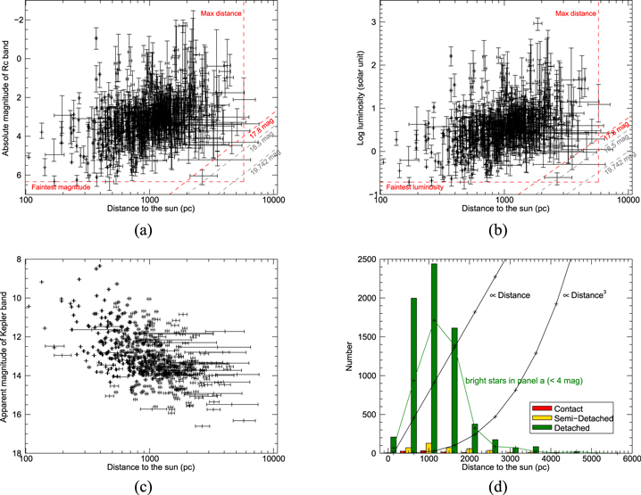
Figure 3. (a) Relationship between the absolute magnitude in the Rc band and the distance to the Sun. (b) Relationship between the luminosity and the distance to the Sun. (c) Relationship between the apparent magnitude in the Keplerband and the distance to the Sun. The slash dashed lines in panels (a) and (b) stand for the apparent limiting magnitude of Kepler spacecraft (19.7 mag) and LAMOST (18.5 and 17.8 mag). (d) Binary distribution along the distance to the Sun. The bars are the distribution for all the stars, and the green line is only for the bright stars (<4 mag in panel (a)) that are detectable up to the max distance line. For comparison, the cases of distribution proportional to the distance (D) and the cubic distance (D3) are shown with black lines. If the binary stars are uniformly distributed in space, the distribution should be proportional to the space volume and so to the cubic distance (D3). It is clear that the samples' distribution is far from the uniform in space.
Download figure:
Standard image High-resolution imageThe limiting magnitude should be the faintest magnitude that both Kepler and LAMOST can reach simultaneously. The faintest magnitude found in the catalog of Kepler eclipsing binary stars is 19.742 mag in Kepler band (KIC 5773205), and LAMOST can reach a limiting magnitude of 18.5 mag in Rc band (Luo et al. 2015). For the stars that were observed by both Kepler and LAMOST (with atmosphere parameters), the faintest magnitude of them is at least 17.8 mag in the Rc band (KIC 9050110 and KIC 10491819) by an incomplete searching. All these limiting magnitudes are shown as slash lines in panels (a) and (b) of Figure 3for the sake of comparison. The adopted limiting magnitude is 17.8 mag (the red slash dashed line), which is probably brighter than the practical limiting magnitude since there are two or three points that lie below it. Therefore, the limiting magnitude of 17.8 mag will overestimate the selection bias on distance by enlarging the area to be corrected. It will be found that this selection bias is rather small, even if it is overestimated.
To correct the selection bias on distance is to calculate how many binaries should be in the red triangle area. This calculation requires the number of stars above the limit line and the distance distribution. How do we know the distance distribution? The most natural and straightforward way is to study the binary samples we already had. Then, the distribution learned can be extended to the outer area, where the number of stars should be calculated to correct this selection bias.
Panel (d) of Figure 3 shows the binary distribution along the distance to the Sun (note that this distribution was already corrected by the first two selection biases). It can be seen that the binaries are mainly found at less than 2000 pc and fade rapidly over larger distances. Accordingly, the number of stars in the distant red triangle area should be small. If the distance distribution was derived from only the bright stars (<4 mag in panel (a)), which are all bright enough to be observed for the whole distance range (0–6000 pc) and so are free of selection bias on distance, the situation is still quite similar (see the green line in panel (d)).
By adopting the distance distribution obtained above and binary samples, the number of stars omitted by the observation in the red triangle area was calculated with the following method. For each binary sample, it may appear at any distance with the probability defined by distribution. The probability P that a binary sample appears on the left side of the limiting line, where the sample is observable, was calculated. Hence, 1–P is the probability of it being at the right side of the limiting line where the sample is not visible. Thereby the number of stars omitted in the red triangle area corresponding to each observed binary sample is  . Hence, the total number of binaries omitted in the red triangle area can be calculated depending on all the binary samples.
It is shown that this correction brings negligible changes. While this situation is in line with our expectations, considering the binary distribution above the limiting line and the small triangle area in the lower right corner.
Even if we use a distribution that can heavily overestimate the selection bias, e.g., a distribution proportional to the distance (see the slash straight black line in panel (d)), the statistical results still make no noticeable difference. In this case, the correction on the selection bias by the distance was not implemented in this work. The number of stars omitted in the small triangle area was negligible.
4.4. The Final Probability for the Correction on the Selection Biases
The final probability for the correction on the selection biases is the product of the first two probabilities, ignoring the negligible affection by distance. The probability for each binary target will be cataloged in Section 5.
It is foreseeable that for the short-period binaries, the probability is close to 100% and goes down with the periods increasing. The longer the orbital periods, the more serious the selection bias. For an illustration, the number of binary targets with periods longer than 1000 days is only 3, but the number after the correction is 1166.5.
5. The Eclipsing Binary Catalog Based on LAMOST and Kepler
As described above, the Kepler spacecraft delivered lots of binary light curves, by which the precise orbital periods, light-curve morphology (used to get the binary subtypes), and phase positions of the secondary minimum (useful for the distribution of orbital eccentricity) were derived. Meanwhile, LAMOST provided the atmosphere parameters for the binary targets, which were assigned to the primary stars. Furthermore, the physical properties were estimated by the help of the isochrone database PARSEC.
According to the Kepler Eclipsing Binary Catalog7 maintained by the Kepler binary group, Kepler observed 3541 binary targets up to 2016 November 14, and 1601 of them were also observed by LAMOST DR4, covering about half of the Kepler targets. Among the 1601 binaries with both observations, 1379 of them were measured with atmosphere parameters successfully, and the remaining 222 failed. The reasons for the failure are the poor spectral quality and the parameters exceeding the limit of the measurement template (e.g., Teff ≲ 3300 K or [Fe/H] > 2.4).
Furthermore, among the 1379 targets with atmosphere parameters, 1320 of them were obtained with physical properties (such as mass, radius, and age) successfully, and 59 were not, which accounts for about 4%. Most of the 59 targets have a surface temperature less than 4000 K. The immediate cause for the failures is that not enough points were found around the targets in the atmosphere parameter space, but the underlying causes were not clear. It is suspected that maybe the errors of some atmosphere parameters are unreasonably small, or the parameters are too extreme to match enough stars in the isochrone database around the targets. Considering the negligible 4%, we hope that this tiny portion of failure does not destroy our statistical results.
A catalog of 1320 binary stars is given in Table 1 deriving from Kepler, LAMOST, and our own calculations with the help of the PARSEC database.
Table 1. Catalog of the Binary Stars Observed by Both LAMOST and Kepler
| KIC Name | R.A. | Decl. | Period | Temperaturea | log ga | [Fe/H]a | Dist.a | Sep. | Morph. | Massa | Radiusa | Agea | Stagea | Prob. |
|---|---|---|---|---|---|---|---|---|---|---|---|---|---|---|
| (J2000) | (J2000) | (days) | (K) | (pc) | (M⊙) | (R⊙) | (yr) | |||||||
| 001026957 | 291.2544 | 36.74361 | 21.7613058 | 4717(92) | 4.650(0.158) | −0.117(0.100) |

|
NaN | 0.01 |

|

|
|

|
0.0303 |
| 001161345 | 291.0487 | 36.83988 | 4.2874555 | 5321(109) | 4.716(0.192) | 0.353(0.107) |

|
NaN | 0.24 |

|

|
|

|
0.1034 |
| 001573836 | 291.5024 | 37.17750 | 3.5570929 | 6698(88) | 4.195(0.133) | −0.273(0.114) |

|
0.4666 | −1.00 |

|

|
|

|
0.1630 |
| 002010607 | 290.5055 | 37.45900 | 18.6322960 | 6249(118) | 3.849(0.230) | 0.092(0.118) |

|
NaN | −1.00 |

|

|
|

|
0.0837 |
| 002012362 | 290.9252 | 37.47633 | 0.3863229 | 6587(156) | 4.304(0.244) | −0.409(0.218) |

|
0.5037 | 0.93 |

|

|
|

|
0.6694 |
| 002167890 | 293.0936 | 37.51451 | 2.6483007 | 4828(103) | 2.701(0.238) | −0.154(0.108) |

|
NaN | 0.29 |

|

|
|

|
0.9548 |
| ⋯ | ||||||||||||||
| A total of 1320 rows | ||||||||||||||
| ⋯ | ||||||||||||||
| 212137767 | 133.6250 | 22.77541 | 15.1779513 | 5275(143) | 3.975(0.287) | −0.053(0.150) |

|
0.5626 | 0.21 |

|

|
|

|
NaN |
| 212145065 | 127.0007 | 22.92870 | 0.3151445 | 5759(133) | 4.379(0.254) | −0.100(0.149) |

|
0.5070 | 0.90 |

|

|
|

|
NaN |
| 212155299 | 126.6134 | 23.14967 | 0.9017195 | 5506(150) | 4.297(0.292) | −0.036(0.162) |

|
NaN | 0.53 |

|

|
|

|
NaN |
| 212159987 | 126.5768 | 23.25371 | 0.7179150 | 7102(176) | 4.134(0.330) | −0.008(0.275) |

|
0.4999 | 0.80 |

|

|
|

|
NaN |
| 212163353 | 134.2129 | 23.33046 | 10.3466173 | 5185(120) | 4.612(0.202) | −0.187(0.137) |

|
0.4986 | 0.11 |

|

|
|

|
NaN |
| 212175535 | 132.5423 | 23.62178 | 0.3223335 | 5573(114) | 4.317(0.227) | 0.278(0.107) |

|
0.4576 | 0.92 |

|

|
|

|
NaN |
Note.
aThe values in parentheses (temperature, log g, and [Fe/H]) are the errors, and the superscript and subscript values (Distance, Mass, Radius, Age, and Stage) are the upper and lower limits of the parameters, respectively.Only a portion of this table is shown here to demonstrate its form and content. A machine-readable version of the full table is available.
Download table as: DataTypeset image
In this catalog, KIC Name, R.A., Decl., and Period are the name, coordinates, and orbital periods of the binary targets taken from the Kepler Eclipsing Binary Catalog. Temperature, log g, and [Fe/H] are the effective temperature, surface gravity acceleration, and metallicity measured from the LAMOST DR4 spectra. They are deemed to stand for the brighter component star (called the dominant luminosity star or primary star) in the binary system as discussed in Section 3.2.
Dist. is the distance of the binary target from the Sun in parsecs taken from Bailer-Jones et al. (2018) based on Gaia parallaxes.
Sep. is the phase separation of the secondary minimum from the primary minimum measured from the light curves which is taken from the Kepler Eclipsing Binary Catalog. If no secondary minimum was found on the light curve, the value is NaN.
Morph. is the morphology of the binary light curve that is also taken from the Kepler Eclipsing Binary Catalog, and it is used to define the binary subtypes roughly. "Values <0.5 are predominantly detached, semidetached are roughly 0.5–0.7, overcontact broadly lie between 0.7 and 0.8 and higher values are a mix of ellipsoidal and uncertain classifications. −1.0 means?" (from http://keplerebs.villanova.edu/search).
Mass, Radius, Age, and Stage pertain to the primary component star of the binary system (see Section 3.3 for details). Stage is the "rough 'evolutionary sections,' 1 = MS, main sequence, 2 = SGB, subgiant branch, or Hertzsprung gap for more intermediate+massive stars, 3 = RGB, red giant branch, or the quick stage of red giant for intermediate+massive stars, 4 = CHEB, core He-burning for low mass stars, or the very initial stage of CHeB for intermediate+massive stars" (from http://stev.oapd.inaf.it/cmd_3.2/faq.html).
Prob. is the probability of the binary target to be a detected eclipsing binary, and it is used to correct the selection bias (see Section 4). Because only the data from the original Kepler mission were used for the correction, and the mission K2 was not used owing to its much shorter observation period. Thus, the targets from K2 (with name headed by number 2) were not calculated for probability and so have no value.
6. The Relationship between the Parameters of the Binary Stars
Since every target has plentiful physical properties, the various correlations between the properties can be investigated. It is expected that some new relationships could be reported. If so, one parameter can be estimated from the other one directly, and the new relationships are helpful for the theory. There are 10 physical parameters in Table 1, which can produce 45 pairs of relationships. The 45 diagrams are too redundant to exhibit them all in this paper, and so only several fundamental relationships related to the period, temperature, and mass are exhibited in Figures 4–6.

Figure 4. Relationship between (a) period and primary star's mass, (b) radius, (c) temperature, (d) metallicity [Fe/H], (e) surface gravity (log g), and (f) the distance from the Sun. Green, yellow, and red stand for the detached, semidetached, and contact binaries, respectively.
Download figure:
Standard image High-resolution imageThe orbital period can be measured accurately without any dependency on the model, so if a parameter has a good correlation with the period, it can be estimated from the period directly. Unfortunately, Figure 4 shows that nearly no parameter has a good correlation with the period. The only good one is the period–temperature relationship on contact binaries, which is actually the well-known period–color relationship.
It can be seen in panel (a) of Figure 5 that the linear correlation is only valid for period ≲0.7 days or primary temperature ≲7500 K, which is consistent with the results of Qian et al. (2017). This relationship can also be reflected by the period–mass diagram (Figure 5(b)), suggesting that the relationship is only valid for the contact binaries with low-mass primary stars (≲1.5 M⊙). Note that the limit 7500 K or 1.5 M⊙ is a coarse boundary between the convective and radiative envelope stars. Thus, the low mass and cool primary stars are mostly convective in the envelope, and the corresponding contact binaries follow the period–color relationship. The contact binaries with massive and hot primary stars with radiative envelopes, however, do not conform with the period–color relationship. Since the fundamental characteristic of contact binaries is the contact of envelopes, the different characters of envelopes arguably lead to different behaviors of them.
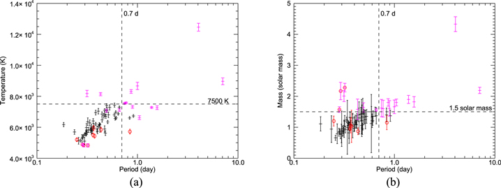
Figure 5. Relationship between (a) period and primary star's temperature and (b) mass for contact binaries. Magenta and red stand for the massive stars (>1.5 M⊙) and post-main-sequence stars, respectively.
Download figure:
Standard image High-resolution imageFigure 6 shows the relationships of some basic parameters. As we can see, the binaries are not uniformly located in all positions but are mostly concentrated in a small area. Moreover, the majority of binaries can be separated from others by a temperature of 7500 K (see panel (b)). Below 7500 K the binaries concentrate in a small area, and above 7500 K the few remaining binaries are spread over a large area loosely. It is interesting that the 7500 K not only can be a limitation on the period–color relationship for contact binaries but also can divide the binaries into two groups.
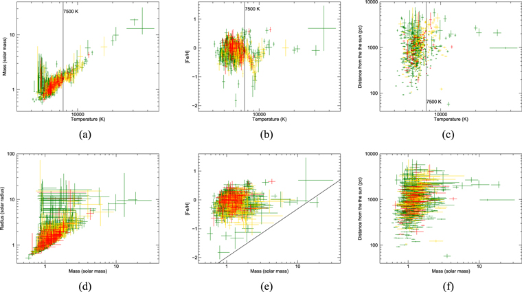
Figure 6. Relationship diagrams for the primary stars on (a) temperature–mass, (b) temperature–metallicity, (c) temperature–distance to the Sun, (d) mass–radius, (e) mass–metallicity, and (f) mass–distance to the Sun. Green, yellow, and red stand for the detached, semidetached, and contact binaries, respectively.
Download figure:
Standard image High-resolution imageThe differences between the binaries separated by 7500 K deserve a reexamination on other binary samples before a theoretical explanation. However, given that the 7500 K is also a coarse dividing line distinguishing two types of envelopes (convective and radiative), this distinction has a physical basis.
In the diagram of temperature–mass (panel (a)), most of the stars follow a linear relationship that mass increases with temperature, which are almost main-sequence stars. Meanwhile, a small number of stars deviate the linear relationship a lot, especially for the stars at the lower left end, which are all post-main-sequence stars. Therefore, this linear relationship is just the mass–temperature relationship for main-sequence stars.
For the mass–metallicity diagram (panel (e)), it seems that there is a lower limit line (the black line), below which there are few targets (if not none). To be more specific, there are rare massive metal-poor binary stars (e.g., binary with [Fe/H] < −0.3 and M > 4M⊙), which is an exceptional phenomenon.
For the diagrams related to the distance to the Sun (panels (c) and (d)), the blank spaces in the lower right area are also an exceptional phenomenon. There are rare massive/hot binaries that were found close to Sun (e.g., binary with M > 4 M⊙ or T > 15,000 K with distance <1000 pc). All the close binaries (<1000 pc) are all lighter than 4 M⊙ and cooler than 15,000 K.
7. The Distributions of the Binary Parameters
Based on the binary catalog with the probabilities for the correction on the selection bias presented in Section 5, the unbiased distribution of binary parameters is obtained. Thanks to the morphology provided by the Kepler binary research group, the distribution of contact, semidetached, and detached binaries can be investigated separately. The binary subtypes, despite being from a coarse classification method, are accurate enough for statistical work. After all, the binaries very close to the border of classification are negligible and so will not have a considerable influence on the whole.
When counting the number of binaries, the reciprocal of the probability is the count for each binary sample. If a binary target has a probability of 0.1, then the count of this kind of target is counted as 1/0.1 = 10. In other words, it is thought that there are another nine binaries with the same parameters but that have not been found photometrically, because they do not eclipse in the line of sight or the eclipse signals were missed by the observation. The lowest probability is 0.0017 (KIC 7672940), which is a 1064.27-day-period detached binary, and it will be counted as 596 binaries in the statistics. The highest probability is almost 1, meaning that the probability of the detectable eclipses is nearly 100%, and it will be counted as one star.
The binary targets studied and exhibited in this section are all from the original Kepler mission (without K2) and are all eclipsing binaries (without noneclipsing binaries). The number of the binary samples from the original Kepler mission is 1070, and within 647 samples are the eclipsing binaries. The reason for excluding the K2 targets is that the observational period of K2 is barely a month, leading to its completeness not being comparable to the original mission. The reason for excluding the noneclipsing binaries is similar, which is that only a few proportions of noneclipsing binaries have been discovered.
Thanks to the distances provided by the Gaia mission (Gaia Collaboration et al. 2016, 2018; Bailer-Jones et al. 2018; Lindegren et al. 2018), the locations of the binary stars in the Galaxy can be depicted (Figure 7). All the binary stars from the original mission of Kepler reside in a quite small and narrow region in the Galaxy disk. In the cylindrical coordinates with the Galactic center as the origin, almost all the binaries have radii between 7000 and 7500 pc and z less than 1000 pc above the Galactic plane. The definition of the Galactic center is R.A. = 17h45m40 04 and decl. = −29°00'28
 1 (J2000 epoch; Blaauw et al. 1960), 7.4 ± 0.3 kpc away from the Sun (Francis & Anderson 2014), and the displacement of the Sun from the Galactic plane is 17 ± 3 pc (Joshi 2007).
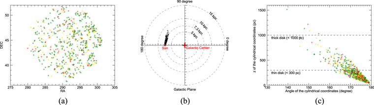
Figure 7. Positions of the stars from the original Kepler mission. (a) Right ascension and decl. at epoch 2000 in the equatorial coordinate system. (b) Locations projected on the Galactic plane. (c) Radius and z in the cylindrical coordinates. Green, yellow, and red stand for the detached, semidetached, and contact binaries, respectively.
Download figure:
Standard image High-resolution image7.1. The Period Distribution of Binaries
Figure 8 shows the period distribution of binaries for the whole (panel (a)) and three subtypes (panels (b)–(d)). The unimodal structure on the logarithmic period for all binaries can be seen unambiguously, and the detached binaries dominate the distribution for its majority amount (panel (b)). The normalized distributions for contact, semidetached, and detached binaries (panel (c)) distinctly demonstrate their differences on period scopes. The distribution on short periods, especially for contact and semidetached binaries, is shown in panel (d) in detail.
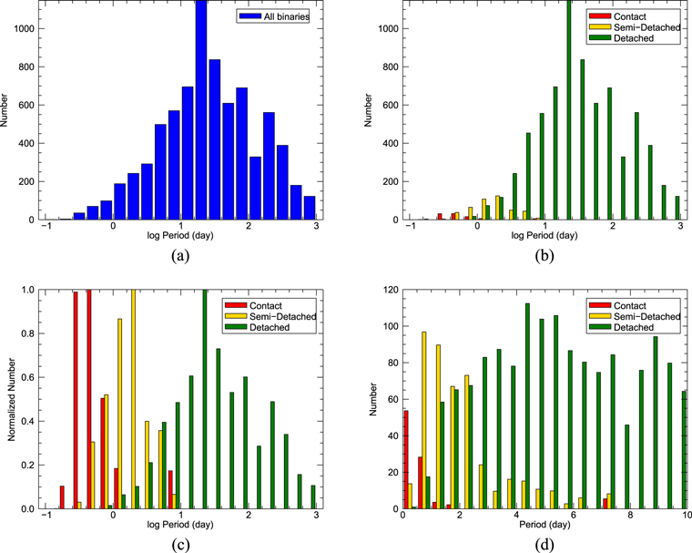
Figure 8. Logarithmic period distribution of the binary stars. (a) Logarithmic period distribution for all the binaries. (b) Same as panel (a), but for detached (green), semidetached (yellow), and contact (red) binaries, respectively. (c) Same as panel (b) but normalized. (d) Same as panel (a), but only for periods less than 10 days and not in logarithm.
Download figure:
Standard image High-resolution imageThe peaks of the distribution for all the binaries and also for the detached binaries are about  corresponding to 20 days, and
  (∼0.4 days) and
  (∼2 days) for the semidetached and contact binaries, respectively. The period distribution is generally smooth, which indicates that the binary sample size is large enough. The two sides of the peak are coarsely symmetrical and monotonous for the detached and semidetached binaries, but for contact binaries a clear cutoff on the lower side at
  (∼0.2 days) can be noticed instantly (panel (c)). Not merely that, but the cutoff is also a cliff just alongside the peak. Despite that the lower-period cutoff for contact binaries is a well-known phenomenon (Rucinski 2007; Li et al. 2019), this statistical diagram is very intuitive and valid based on the new independent data. The proximity of the cutoff to the peak supports the theory of rapid emerges caused by the unstable mass transfer between the two components (Jiang et al. 2012).
The period distribution shown in Figure 8(a) seemingly conflicts with Figure 13 of Raghavan et al. (2010, hereafter R10), which exhibits a unimodal distribution from 259 dwarf and subdwarf stars with a peak at  (∼300 yr) spanning from −1 to 10. R10 carried out a comprehensive search on the ∼F6−K3 stars within 25 pc from the Sun and used various survey methods, from radial velocity searches to the blinking multiepoch archival images, to achieve the completeness.
The period distribution range in this paper is only from −1 to 3, which is a small part of −1 to 10 by R10, but the distribution here presents a prominent unimodal structure instead of a monotonically increasing structure predicted by R10. The explicit contrasts between our results and R10 are probably caused by the following reasons. First, the samples are entirely different. The sample targets in R10 are all located around the Sun within 25 pc; however, the distances of our samples are all larger than 50 pc and up to 12 kpc, averaging over 1 kpc. Second, in order to achieve the complete volume-limited sample, R10 restricted targets by color index (0.5 ≤ B–V ≤ 1.0), brightness (0.1–10 times that of the Sun in V band), and evolutionary stage (with 2 mag above and 1.5 below the main sequence). By contrast, the samples here do not have these restrictions. Third, the samples of R10 originate from different sources, but our samples all come from the Kepler mission. In short, the methods and data of these two works are entirely independent with few similarities.
Does the period distribution depend on the distance from the Sun? Alternatively, does the period distribution vary with the locations in the Galaxy? The answer is probably yes. Figure 9 shows the relationship between distance and period, and it can be seen that the points tend to concentrate around 1000 pc (it should be noticed that the distribution of the points is not corrected on the selection bias because it is a relationship diagram). If the statistics are only carried out on stars with distances less than 500 pc (panel (b)) or larger than 1000 pc (panel (c)), the distribution will be far different from Figure 8(a). Similarly, it is not surprising that the distribution within 25 pc is different from that around 1000 pc. After all, 25 pc is quite small compared to 1000 pc.

Figure 9. (a) Relationship between period and distance. Green, yellow, and red stand for the detached, semidetached, and contact binaries. (b) Same as Figure 8(a), but only for distance less than 500 pc. (c) Same as Figure 8(a), but only for distance larger than 1000 pc.
Download figure:
Standard image High-resolution image7.2. The Age Distribution of Binaries
The age distribution of binaries is displayed in Figure 10. There is a peak at 2–3 Gyr for all binaries (panel (a)) and an excessively high distribution at the right end of 13–14 Gyr. Similar to the period distribution, the detached binaries dominate the distribution (panel (b)), and their peak deviates from that of the semidetached and contact binaries.

Figure 10. Age distribution of the binary stars. (a) Age distribution for all the binaries. (b) Same as panel (a), but for detached (green), semidetached (yellow), and contact (red) binaries. (c) Same as panel (b), but normalized. (d) Ratio of the mean age for semidetached to detached binaries (black) and contact to detached binaries (red) from the Monte Carlo test.
Download figure:
Standard image High-resolution imageBefore the discussion, we need to check the reliability of the distributions first. It is widely known that the age from isochrone interpolation comes with huge errors, and the age errors in this paper are often even larger than the ages themselves. Is the distribution structure shown in Figure 10 generally correct, or just an unreal phenomenon caused by the huge errors? What we need to check is whether the huge errors on age can destroy the distribution shown in Figure 10. The Monte Carlo method was employed for the check, and the result indicates that except for the excessively high distribution at the right end, the other peaks of the distribution and the deviations between them are reliable.
The steps of the Monte Carlo check method are as follows: First, every binary target has an age with a lower and upper limit, which are listed in Table 1. Second, within the error range, a random value is generated to replace the original age for each binary sample. Third, after the two previous steps are finished for all the binaries, a new set of artificial samples on age is created. Fourth, the new sample will make a new age distribution. Fifth, repeat the above steps many times, and a large number of new distributions will be obtained. All the new distributions are checked to see whether the distribution profile displayed in Figure 10 could reappear every time. If some structures (such as peaks, deviations) can always appear on all the new distributions, it indicates that these structures are correct and will not be ruined by the errors. Conversely, if some structures cannot reappear no matter how many new distributions were created, then these structures are not correct. They are just some illusory phenomena caused by the huge errors that heavily influence them.
The result of the Monte Carlo method shows that the excessively high distribution at the right end is not valid for its absence on the new artificial distributions. The other peaks, including the peak at 2–3 Gyr for all binaries and the peaks for the three subtype binaries, are all true.
The unreal excessively high distribution at the right end is caused by the combination of the limitation of cosmic age to 13.8 Gyr and the huge age errors. The interpolated ages often pile up at the upper age limit, leading to an excessively high distribution at cosmic age.
It can be noticed from panel (c) that the peak of detached binaries (2–3 Gyr) is larger than the peak of semidetached and contact binaries (1–2 Gyr), which is an interesting phenomenon to us. In order to examine whether this deviation is real or not, the ratios of the mean ages of semidetached and contact binaries to those of detached binaries are shown in panel (d) from 5000 times Monte Carlo tests. Every point in panel (d) represents an individual test, and it can be recognized that all the points are below 1 with an average of ∼0.65, indicating that the mean ages of semidetached and contact binaries are positively lower than those of detached binaries, despite the huge errors.
Although the mean age deviation is not a false phenomenon caused by the errors, is it realistic in physics? In other words, are the semidetached and contact binaries actually younger, or do they merely look younger compared to the detached binaries? Because the ages were derived by the isochrone interpolation method that originates from the single-star model, an essential premise is that the stars are independent of other stars in evolution (such as no mass transfer). However, for the evolution of a binary system, the mass transfer is commonly seen. So the age derived from atmosphere parameters is not positively realistic.
If a star accretes mass from others, its age measured from the atmosphere based on the single-star model will be younger than its actual age. To illustrate this problem, let us use an example. Assume that there are two stars, MA = 1 M⊙ and MB = 1.5 M⊙, that were born at the same time. It is conceivable that the burning speed of the core hydrogen of MA is much slower than that of MB. After a period of time, MA accretes 0.5 M⊙ mass from elsewhere, making MA be 1.5 M⊙ that is as massive as MB. Although the masses are the same, their atmosphere and cores are different. The burned central hydrogen of MA is smaller than MB, so the apparent age of MA by its atmosphere is younger than the age of MB, which is also the actual age of MA.
For the current primary stars of the contact or semidetached binaries, it is a typical case to accrete half of their original mass from their companions during the evolution history. According to our calculations, the mass gainer star will accrete at least 20% of its original mass. Therefore, the current primary stars in contact or semidetached binaries will look much younger from the atmosphere than their actual ages.
For the detached binaries, there was no mass transfer, and so the evolution of their component stars is similar to that of single stars. Thus, their ages by the atmosphere are generally the actual ages.
The ages displayed in Figure 10 are all estimated from the primary stars' atmosphere, which are the apparent ages instead of the actual ages. Although the apparent ages of contact and semidetached binaries are much younger compared to detached binaries, their actual ages are not certainly younger. It cannot be ruled out that the semidetached and contact binaries have the same average age as the detached binaries. The semidetached and contact binaries only look much younger than their actual ages owing to huge mass transfer in the evolutionary history.
The average apparent age of the contact binaries equals that of the semidetached binaries, suggesting that the contact binaries experienced the same amount of mass transfer as the semidetached binaries, and also suggesting that nearly all the contact binaries originated from the semidetached binaries when the mass transfer took place.
The average age of detached binaries in Figure 10 represents the actual age of the whole binaries, with a peak value of 2–3 Gyr and a mean value of ∼5 Gyr, which is close to the solar age.
7.3. The Mass, Radius, Temperature, and Metallicity Distribution of Binaries
The mass, radius, temperature, and metallicity distribution of binaries are exhibited in Figure 11. Although the global distribution for all the binaries is not presented here, the distribution of detached binaries shown in the left panels can represent the whole binaries owing to their dominated number. The distributions of the three subtypes of binaries are similar (middle panels), but their small differences can still be extracted by the Monte Carlo method (right panels). Similar to the work on age distribution above, the same test was carried out on other parameters. It can be observed that compared to the detached binaries, the semidetached and contact binaries are 10%–15% larger on mass and temperature (note that all the parameters belong to the dominant luminosity component star, also called the primary star). The radius and metallicity of the contact binaries may be a little bit higher than those of semidetached binaries, but both close to the detached binaries.
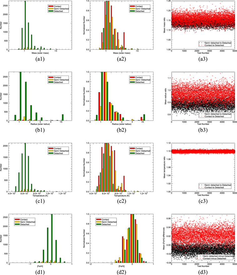
Figure 11. Mass (a1)–(a3), radius (b1)–(b3), temperature (c1)–(c3), and metallicity [Fe/H] (d1)–(d3) distribution of the binary stars. Left panels: distribution of detached (green), semidetached (yellow), and contact binaries (red). Middle panels: same as left panels, but normalized. Right panels: ratio/differences of mean values for semidetached to/minus detached binaries (black) and contact to/minus detached binaries (red) from the Monte Carlo test.
Download figure:
Standard image High-resolution imageThe similarity and difference of the distributions between three subtypes of binaries provide some clues on their circumstances of birth. Considering that the metallicity of different subtypes of binaries is close to each other, and the metallicity almost maintains the initial value, the different subtypes may not have any difference in their circumstances of birth.
Although the differences in mass and temperature are evident, these differences cannot reflect the past situation because the semidetached and contact binaries both experienced lots of mass transfer, causing the current primary star to be far different from the original ones. The deviation on age distribution, as discussed above, may only indicate the substantial mass transfer in the evolutionary process and thus cannot reflect the environment of birth. The only difference directly related to birth is the period distribution, but they are in line with the definition of the binary subtypes.
To sum up, no parameter can support differences in the birth environment for the three subtypes of binaries. The difference in period distribution may suggest that the formation of a binary system is merely a random process. All the binaries are formed as detached binaries in the beginning, and for those two components that happened to be very close to each other on birth will quickly evolve to be semidetached binaries, and part of them will further evolve to be contact binaries.
7.4. The Orbital Eccentricity Distribution of the Detached Binaries
For the semidetached and contact binaries, their orbits are always circular owing to the strong tidal friction. However, for the detached binaries, especially the long-period binaries, their orbits are often eccentric. The orbital eccentricity for each binary is unknown because the light-curve modeling was not carried out. Despite that, the eccentricity distribution of all the detached binaries can be calculated. The method is to utilize the precise phase positions of the secondary minima to restrict the eccentricities.
By using the secondary minimum position, a formula consisting of eccentricity e and longitude of periastron ω can be calculated, that is,  (Kopal 1959, page 385). Just like a parameter, the distribution of this quantity is obtained (Figure 12(a)). Since the coupling distribution of e and ω is known, and if the distribution of ω is known as well, the distribution of e can be acquired by the Monte Carlo method.

Figure 12. Distributions of the detached binaries on (a)  , (b) eccentricity e, (c) the relationship between age and minimum eccentricity, and (d) the relationship between period and minimum eccentricity (d).
Download figure:
Standard image High-resolution imageThe ω can be assumed to be uniformly distributed between 0 and 2π, so the distribution of e can be obtained. First, for each known  , a random ω is assigned to it, and then the e can be worked out directly. Second, repeat the first step with many random ω, and then many e were generated. The distribution of all the artificial e is the distribution of the binary eccentricity, which is shown in Figure 12(b).
In order to avoid the problem by the inadequate number of random values that is caused by the limited number of binary targets, the original sample is expanded 1000 times, namely, from the original 4588 (after the correction of selection bias) to 4,588,000. To make sure that the number of random values is adequate, the calculation was repeated 10 times to generate 10 distributions of e, and no difference can be identified between them by the naked eye. This indicates that the distribution obtained is the only one that conforms to the observations.
The distribution of e shows a continuous decline starting from a notable high distribution at e = 0–0.1. A considerable number of detached binaries with circular orbits is a direct reflection of the orbital circularization by the ongoing tidal friction. The sudden rise around e = 1 is quite an unexpected phenomenon to us and might reveal some new unrecognized evolutionary process if this phenomenon is believable. The detailed distribution at e = 0.9–1 is enlarged in a subpanel. There is a slow upward trend from 0.90 to 0.99 and a surprising jump at 0.99–1. Similar to the case at e = 0, binaries seem to accumulate at e = 1 but in a much small degree. For this strange distribution, we are unable to give a reasonable interpretation.
Although the eccentricity of each binary target is unknown, a lower limit of the eccentricity can be calculated by setting  in the known
  . We wish that the minimum value of the eccentricity could promote the understanding of the eccentricity distribution.
The relationship between the lowest eccentricity and the age/period is shown in panel (c)/(d), and there is no definite correlation that can be recognized. Although it is intuitive that the older the age, the higher the degree of orbital circularization, the actual outcome is not evident. It can be regarded in panel (d) that the longer the period, the wider the range of the lowest eccentricity (note that the point distribution is not corrected for selection bias and so cannot stand for the actual distribution).
Why are the long-period binaries more likely to have large eccentricity orbits? If we assume that the two component stars are formed together within the same piece of a molecular cloud, their initial orbital eccentricity should be zero at birth owing to the strong friction within the dense cloud accompanying the accretion process. The reason for the high odds of large eccentricity on long-period binaries may be the interference from other bodies because the wide and hence the loose binaries are more susceptible to being gravity disturbed by the outer bodies.
7.5. The Evolutionary Stage Distribution of Binaries
The roughly evolutionary stage distribution of binaries is also obtained (see Figure 13). Similar to the case of mass, radius, and temperature, this evolutionary stage connects to the primary component in the binary system.
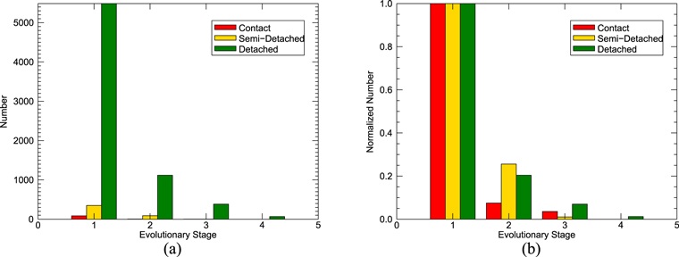
Figure 13. Evolutionary stage distribution of the binary stars. (a) Distribution for detached (green), semidetached (yellow), and contact binaries (red). (b) Same as panel (a), but normalized. The evolutionary stages are (1) main sequence; (2) subgiant branch, or Hertzsprung gap for more intermediate+massive stars; (3) red giant branch, or the quick stage of red giant for intermediate+massive stars; (4) core He burning for low-mass stars, or the very initial stage of CHeB for intermediate+massive stars.
Download figure:
Standard image High-resolution image
The majority of the primary stars are in the main-sequence stage, and the distribution decreases when the stage goes higher, which fits our expectation. It is worth mentioning that the proportion of the post-main-sequence stage of contact binaries (10%) is much lower than that of semidetached (21%) or detached (28%) binaries. First of all, it is consistent with our observational experience that contact binaries are frequently main-sequence stars. Moreover, it seems to imply that post-main-sequence contact binaries cannot live for a long time as the detached and semidetached binaries. If one component star in a contact binary evolved beyond the main sequence, it would reasonably experience a process of rapid expansion. During the rapid expansion, the evolved star is likely to devour its companion, becoming a single star. However, for primary stars in detached or semidetached binaries, their Roche lobe is probably large enough to accommodate the expansion.
8. Summary and Conclusion
Based on the LAMOST and Kepler database, a statistical work on binary stars was carried out. Because of the superior features of these two surveys and their complementary advantages, the binary samples are endowed with distinguished characteristics. A catalog of 1320 binaries was presented by crossing the two surveys. Each target in this catalog has unprecedented light curves and high-quality spectra. Along with the parameters that can be directly measured out from the observations (such as orbital periods, binary subtypes, and atmosphere parameters), the physical properties (such as mass, radius, and age) of the primary stars were also presented with the help of the PARSEC isochrone database.
The plentiful parameters allow us to study relationships between various parameters. The relationship diagrams between the period and the other six parameters were studied, yet none of them exhibit an obvious correlation. The only good correlation is observed between temperature and period for the contact binaries, which is widely known as the period–color relationship.
Careful analysis shows that the good linear relationship is only valid for periods shorter than 0.7 days, and only for main-sequence stars cooler than 7500 K. This relationship can also be expressed in terms of period and primary mass. From another point of view, the period–color relationship conforms only to low-mass (<1.5 M⊙) main-sequence stars.
The temperature–color relationship is substantially the correlation of mass, radius, and temperature for main-sequence stars under the configuration of contact binaries. In this case, what we need to study is not the reason for the period–color relationship for low-mass main-sequence stars, but why the relationship cannot fit massive stars in contact binaries. Considering that the dividing line of temperature/mass approximately corresponds to the boundary of the convective and radiative envelope, together with the common envelope structure in the contact binary systems, the reason may correlate with the insufficient energy exchange efficiency in the radiative common envelope.
The relationship concerning the temperature and mass was presented. The temperature and mass form a linear relationship for main-sequence stars. It is recommended that the temperature 7500 K can divide the binaries into two groups. Below 7500 K the binaries are concentrated with low dispersion on temperature and metallicity, and above 7500 K binaries lie in a broad range loosely. Because 7500 K is approximately the dividing line between the convective and radiative envelope, the classification of the two groups probably makes sense physically.
A lower limit was proposed in the relationship between primary mass and metallicity showing that the massive stars (>4 M⊙) are almost metal-rich ([Fe/H] > −0.3).
Interestingly, the temperature and mass appear to depend on the distance between the binaries and the Sun. This situation implies that the binary distribution may vary with distance, or, say, vary with different locations in the Galaxy disk. Massive or hotter binaries (>15,000 K or 4 M⊙) are very probably distant from the Sun (>1000 pc).
The source of the binary samples used for statistics is unitary (all from Kepler observations in a fixed field of view for more than 1000 days) and thorough (all observed eclipsing binaries were discovered). As a result, it is feasible to correct the selection bias and to offer an unbiased distribution on binary parameters.
To correct the selection bias, the prior distributions of four parameters need to be assumed, and the reliability of the assumptions could heavily influence the statistical results. For the orbital inclination, the longitude of periastron, and the position of the eclipse occurring at the timeline, their assumptions on the distribution are very natural, i.e., these three parameters are randomly and uniformly distributed.
The only problem is the distribution of the mass ratio. In this paper, the exponential distribution is assumed as in Tian et al. (2018) and Raghavan et al. (2010), and the coefficient 0.3 is somewhat arbitrary. This distribution introduces the major uncertainty on the results. The fundamental solution requires comprehensive radial velocity measurements, or at least the light-curve analysis on all the Kepler eclipsing binaries. Either of them is a tremendous amount of work but unavoidable.
The orbital period distribution of binary stars is obtained, spanning from  to 3 with a peak at
  . This distribution is quite different from R10, where the peak is
  . However, this divergence is most likely caused by the nonuniform distribution on distance or the small sample size.
Because our binary targets (as well as the targets of R10) are located in a rather small area in the Galaxy disk, it is irresponsible to generalize the statistical results to the entire Galaxy disk. The differences by the distance from the Sun may be attributed to the intrinsic nonuniform distribution of the binaries themselves, but they may also be just a fictitious phenomenon caused by the small sample size.
The lower period cutoff ( days) for contact binaries was intuitively exhibited. Besides, this cutoff is adjacent to the highest point of the period distribution. This phenomenon fully supports the conclusion that the contact binaries evolve toward the shorter period and quickly disappear (by merging into single stars) after crossing a period cutoff value (
 days).
The "apparent" mean ages of semidetached and contact binaries are much younger than their actual ages, as well as much younger than the actual age of the detached binaries. The "apparently" young age of semidetached and contact binaries indirectly supports the huge mass transfer during their evolution and implies that there may be no statistical difference in age for all subtypes of binary stars. Furthermore, the amount of mass transfer experienced by contact binaries is approximately equal to that of semidetached binaries, or, say, the mass transfer during the contact stage is marginal. It also suggests that almost all the contact binaries are evolved from the semidetached binaries.
For contact binaries, in addition to the cutoff on period, there is a truncation on the temperature of about 7500 K. The temperature distribution (Figure 11, panel (c2)) showed that the number of contact binaries hotter than 7500 K drops suddenly. The boundary 7500 K can be noticed not only in the temperature relationship diagrams but also in the distribution diagrams. It might be meaningful to classify the binaries (especially the contact binaries) into two groups by 7500 K and to study them separately.
All the distributions of parameters except period are roughly consistent with each other between contact and semidetached binaries, which can be viewed at both distribution diagrams and the mean ratio diagrams. This suggests the similarity on the formation and evolution between the contact and semidetached binaries.
For the first time, the orbital eccentricity distribution of the detached binaries was presented, although the eccentricity of each binary target is still unknown. With the increase of eccentricity, the distribution decreases gradually. However, the distribution goes up suddenly when eccentricity approaches 1 (>0.99). It is a shocking result to us, and it deserves further examination. Although time will promote the orbital circularization, no correlation is noticed between the eccentricity and the age.
High eccentricities are more frequent in longer-period binaries, most likely because the long-period binaries are more fragile in response to the gravitational interference from outer bodies.
The distribution of the rough evolutionary stages was presented. The proportion of post-main-sequence contact binaries is relatively much lower, suggesting that they are not long-lived compared to the semidetached or detached binaries.
In the end, the statistical comparison of different subtypes of binary stars can give us some information on their evolution and formation. The metallicity distributions of the three subtypes of binary stars are very similar, suggesting that all the binaries may have been born at a similar circumstance. The reason for their current subtypes may be simply the random separation distance between the components at birth. Regardless of the initial separation, all binary stars are detached at birth. Those with very close separation will quickly become semidetached or further contact binaries, leaving the majority of binaries to remain in their detached configuration.
We thank the anonymous referee very much for his/her help on both science and language. We are indebted to the Kepler Science Working Group on Eclipsing Binaries for all their great pilot works that have made such discoveries possible.
All of the data presented in this paper were obtained from the Guoshoujing Telescope and the Kepler mission. The Guoshoujing Telescope (the Large Sky Area Multi-Object Fiber Spectroscopic Telescope, LAMOST) is a National Major Scientific Project built by the Chinese Academy of Sciences. Funding for the project has been provided by the National Development and Reform Commission. LAMOST is operated and managed by the National Astronomical Observatories, Chinese Academy of Sciences. Funding for the Kepler mission is provided by the NASA Science Mission directorate. This work presents results from the European Space Agency (ESA) space mission Gaia. Gaia data are being processed by the Gaia Data Processing and Analysis Consortium (DPAC). Funding for the DPAC is provided by national institutions, in particular the institutions participating in the Gaia MultiLateral Agreement (MLA). The Gaia mission website is https://www.cosmos.esa.int/gaia. The Gaia archive website is https://archives.esac.esa.int/gaia.
This work is supported by the Chinese Natural Science Foundation (grant Nos. 11703082, 11703080, 11933008, and 11403056) and the Yunnan Natural Science Foundation (No. 2018FB006).
Facilities: LAMOST - , Kepler. -
Footnotes
- 5
β Persei was the first variable object recorded by ancient Egyptians before 1163 B.C., which is a triple-star system by later study.
- 6
The field of view is fixed in the original mission. For mission two, called K2, the field of view changes every ∼80 days.
- 7