


Abstract
The observation of the non-Keplerian behavior of propeller structures in Saturn's outer A ring raises the question: how does the propeller respond to the wandering of the central embedded moonlet? Here, we study numerically how the structural imprint of the propeller changes for a libration of the moonlet. It turns out that the libration induces an asymmetry in the propeller, which depends on the libration period and amplitude of the moonlet. Further, we study the dependence of the asymmetry on the libration period and amplitude for a moonlet with a 400 m Hill radius, which is located in the outer A ring. This allows us to apply our findings to the largest known propeller Blériot, which is expected to be of a similar size. For Blériot, we can conclude that, supposing the moonlet is librating with the largest observed period of 11.1 yr and an azimuthal amplitude of about 1845 km, a small asymmetry should be measurable but depends on the moonlet's libration phase at the observation time. The longitude residuals of other trans-Encke propellers (e.g., Earhart) show amplitudes similar to Blériot, which might allow us to observe larger asymmetries due to their smaller azimuthal extent, allowing us to scan the whole gap structure for asymmetries in one observation. Although the librational model of the moonlet is a simplification, our results are a first step toward the development of a consistent model for the description of the formation of asymmetric propellers caused by a freely moving moonlet.
Export citation and abstract BibTeX RIS

Original content from this work may be used under the terms of the Creative Commons Attribution 3.0 licence. Any further distribution of this work must maintain attribution to the author(s) and the title of the work, journal citation and DOI.
1. Introduction
Planetary rings are the most beautiful structures in our solar system and are mainly composed of differently sized icy particles. The dense main rings of Saturn are composed of particles ranging from centimeters to a few meters (Cuzzi et al. 2018), and beside this ensemble of particles, even larger boulders (called moonlets) orbit within the ring environment. The moonlet interacts with the surrounding ring material gravitationally and opens a partial gap around its orbit. The different angular speeds at different semimajor axes affect the shape of the created gap, resulting in the inner gap—due to the higher angular speed of the ring material—overtaking the embedded moonlet while the outer one falls behind. Viscous diffusion of the ring material counteracts this gravitational scattering process and, thus, results in a closing of the opened gap with a growing azimuthal distance to the embedded moonlet (Spahn & Sremčević 2000; Sremčević et al. 2002; Seiß et al. 2005; Hoffmann et al. 2015). For a moonlet larger than a critical radius, its gravity compensates the viscous diffusion along the whole circumference of the orbit and, thus, the gap is kept open. For smaller moonlet radii, the gravity of the moonlet does not suffice to compensate for the viscous diffusion and, therefore, the gap closes. As a result, two partial gaps inside and outside the orbit of the moonlet decorated with wakes remain and resemble an S-shaped, two-bladed propeller. Those propellers act as structural insignia to detect the embedded moonlet in the dense rings.
After the postulation of their existence in Saturn's rings to explain optical depth variations in the Voyager data (Henon 1981; Lissauer et al. 1981), the cameras on board the spacecraft Cassini finally revealed their presence within the dense rings of Saturn (Tiscareno et al. 2006, 2008; Sremčević et al. 2007). Meanwhile, different populations of propeller structures inside Saturn's A ring have been identified in the images. Between 127,000 and 132,000 km from Saturn's center, three propeller belts have been observed, which contain several thousand propellers, all being generated by moonlets of radii ≲0.15 km (Tiscareno et al. 2008). Further outward, between the Encke and Keeler gap, about 37 larger propellers that are created by moonlets with radii between ∼0.15 km and ≲1.0 km have been found (Tiscareno et al. 2010). Due to their relatively large sizes, 11 of these giant propellers were able to be identified in different subsequent images, allowing the reconstruction of their orbital motion. The analysis of their orbital evolution revealed a longitudinal deviation from their expected Keplerian location—called excess motion (Tiscareno et al. 2010; Spahn et al. 2018).
The largest propeller structure is called Blériot and is created by a moonlet of about 400 m in the Hill radius (Hoffmann et al. 2016; Seiß et al. 2019). Its excess motion can be reconstructed by a superposition of three sinusoidal harmonics with periods of 11.1, 3.7, and 2.2 yr and amplitudes of 1845, 152, and 58 km with a standard deviation of about 17 km of the remaining residual (Seiler et al. 2017; Spahn et al. 2018). Blériot's excess motion resembles the typical librational motion of a resonantly perturbed moon (Goldreich 1965; Goldreich & Rappaport 2003a, 2003b; Spitale et al. 2006; Cooper et al. 2015) and, thus, supports the hypothesis that this excess motion might result from a resonant or near-resonant driven by one or several of the outer satellites. Numerical simulations1 have shown that the collective perturbation by the outer satellites Prometheus, Pandora, and Mimas is able to induce correct libration frequencies to explain the three mode fit, but the induced libration amplitudes are far too small to explain the observations (Seiler et al. 2017).
Alternatively, a stochastic migration of the embedded moonlet due to collisions or density fluctuations in the rings has been proposed as well (Crida et al. 2010; Pan & Chiang 2010, 2012; Rein & Papaloizou 2010; Pan et al. 2012; Bromley & Kenyon 2013; Tiscareno 2013). The most promising results have been obtained by Rein & Papaloizou (2010), who considered a random walk in the semimajor axis of the moonlet. In N-body simulations, Pan et al. (2012) were able to generate an amplitude in the moonlet's excess motion of about 300 km over a time span of 4 yr. Nevertheless, their resulting amplitude is also too small.
In order to solve this amplitude problem, Seiler et al. (2017) suggested a propeller–moonlet interaction model, where the usually assumed point symmetry of the propeller structure is broken by a slight displacement of the central moonlet. This breaking of the point symmetry causes a restoring force toward the moonlet, resulting in a harmonic oscillation in the moonlet's mean longitude. The libration depends on the physical parameters of the propeller and the surrounding ring material. This oscillating system has its own eigenfrequency so that for an external resonant driving with a frequency, which is sufficiently close to the eigenfrequency of the propeller–moonlet oscillator, an originally small libration mode can be amplified by several orders of magnitude.
However, the suggested propeller–moonlet interaction model oversimplifies the physical problem in the aspect that it reduces the gap structures to two radially separated rectangular-shaped boxes with fixed azimuthal end points, where the beginning of the gap follows the moonlet motion. Further, the surface mass density inside these boxes is assumed to be constant. In reality, the gap structure has an azimuthal extent of up to several thousand kilometers, and the surface mass density within the gap structure is a decay rather than constant. Due to the radial separation of the gaps from the moonlet, the perturbation caused by the moonlet's motion first needs time (set by the Kepler shear) to be transported along the gap structure. Thus, the perturbation by the moonlet's motion only arrives at the gap ends after a certain delay time (hereafter called Tgap), while the beginning of the gap more or less follows the moonlet motion instantaneously. For Blériot, this delay time would be about Tgap ≈ 0.5 yr considering a gap length of 6500 km, respectively (Seiler et al. 2017).
As a consequence of the moonlet's wandering and the delayed reaction of the gap ends, we expect the gap structures to become asymmetric. In this article, we test this expectation numerically for a given (forced) moonlet libration, where we consider the moonlet libration as given and do not study its origin. In contrast to the propeller–moonlet interaction model (Seiler et al. 2017), we consider the moonlet's libration amplitude and period as variables to study the dependence of the asymmetry on the moonlet libration and to answer the question whether such an asymmetry might be detectable in Cassini Imaging Science Subsystem (ISS) images. Therefore, we search the simulated gap structures for properties, which allow a direct measurement of the asymmetry.
The plan of this paper is as follows. First, we give an overview of our hydrodynamic simulation code and how we model the moonlet libration (see Section 2). Afterward, we present the results of our simulations and show how the appearance of the propeller and the different properties of the gap structures change with the libration of the moonlet. For this purpose, we directly compare our results to simulations of a symmetric propeller structure (see Section 3). The propeller–moonlet interaction model predicts that the restoring force by the gap-asymmetry follows the moonlet motion. This hypothesis is checked against our simulation data (see Section 4). As a next step, we study the dependence of the asymmetry on the libration period and amplitude and test under which conditions the asymmetry becomes detectable (see Section 5). Based on our analysis, we apply our findings to the propeller Blériot in Section 5.3. In the end of this paper, we conclude and discuss our findings (see Section 6).
2. Hydrodynamic Simulation
Our hydrodynamic simulation routine is based on the code developed by Seiß et al. (2019). This integration routine will be modified so that the moonlet can librate around its mean orbital position within the simulation grid.
We consider a moonlet embedded in the granular environment of Saturn's rings with a surface mass density of Σ. The evolution of the surface mass density is described by the continuity equation,

and the momentum balance is quantified by the Navier–Stokes equation,

Both equations above are presented in the flux conserved form, where the tensor product is denoted by the ◦ symbol. The symbol ∂t = ∂/∂t denotes the partial time derivative. The gravitational potentials of the central planet and the moonlet are described by Φp and Φm. Further, we choose our simulation's coordinate system to corotate with the moonlet's mean orbital frequency,  , where G and Mp denote the gravitational constant and the mass of the central planet and are centered at the moonlet's mean radial position, r0. The right-hand side term
  i in the Navier–Stokes equation contains the centrifugal and Coriolis forces in the corotating frame given by

Here, we neglect the oblateness of Saturn.2
In comparison to their radial and longitudinal extent (several hundred thousand kilometers), the vertical dimension (≲100 m) of Saturn's rings is tiny. Thus, Equations (1) and (2) can be reduced to a two-dimensional problem using vertically integrated quantities (Spahn et al. 2018). Additionally, the moonlets in the outer A ring are expected to revolve on nearly circular orbits (ae ≲ 1 km) in the equatorial plane of Saturn.
In comparison to the spatial extent of the rings, the propellers are tiny. As a consequence, only a small ring area centered around the moonlet's orbital position needs to be considered for our simulations. Therefore, the acting forces in the vicinity of the moonlet can be linearized and described by the Hill problem (Hill 1878). Here, we choose x to represent the radial distance from the moonlet and y stands for the azimuthal direction. As a result, the gravitational potential of the central moonlet is given by

with  as the smoothing radius, which limits the gravitational potential in the close vicinity of the moonlet's center. Here, we choose = 0.2 h. The mass of the moonlet, Mm, defines its Hill radius as
where a0 denotes the semimajor axis of the moonlet's mean orbit.
We treat the granular ensemble forming dense rings as a usual (linear) fluid. Thus, the pressure tensor,  , can be described with the Newtonian ansatz as
where p, ν, and ξ denote the scalar pressure, the kinematic shear, and the bulk viscosities, respectively. The dependence of the pressure and the viscosities on the local density can be described by the power laws (Spahn et al. 2000)
Additionally, we set the ratio between shear and bulk viscosity constant as

In the simplest case, the unperturbed pressure is given by the ideal gas relation, p0 = Σ0  , at equilibrium, where c0 denotes the dispersion velocity. In our simulation scheme, we use an isothermal model and, therefore, the dispersion velocity, c0, and the related granular temperature, Tgr =
  /3, are constant.
2.1. Methods
The simulation area is a rectangular cut out of the ring environment of dimensions (xmin, xmax) and (ymin, ymax), which is centered around the mean orbital position of the moonlet. This box is divided into Nx × Ny equal-sized cells (see Table 1). The complete set of equations is integrated until a steady state is established. The advection term is solved with the second-order scheme with "MinMod" flux limiter (LeVeque 2002) in order to better conserve the wake crests. The influence of pressure and viscous transport is solved with an explicit scheme. At the borders of the calculation regions, the boundary conditions are chosen such that the perturbations can flow out of the box freely, while the inflow is unperturbed. This is especially important at the azimuthal boundaries, where, due to Kepler shear, the material is flowing into the box at x < 0, y = ymin and x > 0, y = ymax and flowing out at x < 0, y = ymax and x > 0, y = ymin. The influence of the moonlet is established mainly by its gravity.
Table 1. Simulation Parameters for the Hydrodynamic Simulation
| Parameter | Value |
|---|---|
| Scaling parameters: | |
| h | 400 m |
| Ω | 1.3 × 10⁻⁴ s−1 |
| ν0 | 300 cm2 s−1 |
| c0 | 0.5 cm s−1 |
| Σ0 | 400 kg m−2 |
| Ring parameters: | |

|
1.441 × 10⁻³ |

|
4.811 × 10⁻² |
| α | 1 |
| β | 2 |

|
7 |
| Box parameters: | |
| xmin | −10 h |
| xmax | 10 h |
| ymin | −800 h |
| ymax | 800 h |
| Nx | 400 |
| Ny | 6400 |
Note. Those parameters are used for the scaling, viscosity, and simulation area within the integration routine.
Download table as: ASCIITypeset image
A more detailed overview of the implementation of the integration routine and the numerical methods is given in Section 3 in Seiß et al. (2019).
Internally, our simulation routine uses scaled (unitless) values, where lengths and times are scaled by the Hill radius, h, and mean motion, Ω, of the moonlet, while throughout this work, lengths and time are measured in Hill radii and orbits. Further, we scale the surface mass density by its unperturbed value, Σ0, for which we use 400 kg m−2 (Colwell et al. 2009). Here, we will focus on the asymmetry formation for the giant trans-Encke propellers. For this reason, we will consider a Blériot-sized moonlet with a 400 m Hill radius (Hoffmann et al. 2016; Seiß et al. 2019), allowing us to predict the asymmetry of its propeller. Therefore, we will simulate the moonlet at a radial location close to its observed orbital position, and we will adopt the viscosity accordingly (Seiß et al. 2019). The set of used parameters and their values—if nowhere else mentioned—is given in Table 1.
The simulation code uses scaled viscosities and sound speed due to the length and time scaling:


Their values and further simulation parameters are given in Table 1.
2.2. Modeling the Moonlet Motion
We model the moonlet libration as a slow radial libration in the semimajor axis of the moonlet  . This radial change results in a slow drift influencing the moonlet's mean motion, which further is related to the azimuthal position of the moonlet

Thus, the modeled moonlet motion is given by


where ωm = 2π/Tm is the libration frequency of the moonlet. The radial amplitude and the libration period of the moonlet are denoted by xm,0 and Tm.
3. Visualization of the Asymmetry
For the presentation of our simulation results, we will define and analyze different characteristics of the propeller shape and directly compare the results for a symmetric and an asymmetric propeller. In this way, we show how the asymmetry of the propeller can be characterized. Our results have been obtained for a moonlet with a 400 m Hill radius. For the asymmetric propeller—if nowhere else mentioned—the moonlet has been forced to librate around its mean orbital position with a radial amplitude of xm,0 = 0.5 h and a period of Tm = 80 orbital periods. The value of the radial amplitude (xm,0 = 0.5 h) is motivated from the longitudinal excess motion of Blériot (Seiler et al. 2017; Spahn et al. 2018), which is of a similar size (see Section 5.3).
3.1. Density Profile
The typical imprint of an unperturbed propeller structure, where the moonlet (represented by the star symbol) is not librating, is shown in the top left panel of Figure 1. A clear symmetry can be seen. The gray scale color code illustrates the scaled surface mass density, where darker color corresponds to regions of depleted density, while brighter color represents denser regions. The x and y directions in the presented plots denote the radial and azimuthal distances to the mean orbital position of the moonlet. For a better visualization, the presented area around the propeller is reduced radially and azimuthally to Δx = ±6 h and Δy = ±600 h.

Figure 1. Comparison of a symmetric propeller (top left) and two examples of an asymmetric propeller (bottom panels). The two asymmetric examples show the propeller for a librating moonlet at the same libration phase, but for different libration periods (see the top right panel). In the bottom left panel, the moonlet is librating with Tm = Tgap, while in the right panel, the period is Tm = 3 × Tgap. In all panels, the origin of the coordinate system is centered to the mean orbital position of the moonlet. The moonlet's actual position is given by the star symbol. In all cases, the moonlet's Hill radius is h = 400 m and its libration amplitude was set to xm,0 = 0.5 h. The black lines denote the density profile at a 80% gap relaxation.
Download figure:
Standard image High-resolution imageFresh inflowing material (moving from left to right) passing by the by the moonlet from the inside at Δx < 0 are more deflected to the moonlet the closer they pass it radially. The same mechanism applies for freshly inflowing material on higher orbits than the moonlet (Δx > 0), where the lower angular speeds yield a material flow from right to left. For larger radial distances, this deflection decreases as  . This induces a coherent motion of the ring material and, thus, results in the formation of wakes. The location of the moonlet within the simulation grid, which is centered on its mean orbital location, is illustrated by the star symbol. Further, the black line marks the propeller surface mass density level at 80% of gap closing (Σ/Σ0 = 0.8). At this level of the surface mass density, a clear symmetry can be seen when comparing the inner and outer gap region, where the gap lengths are about 540 h and the maximum gap widths are about 2 h, respectively.
This symmetry is broken in the bottom panels of Figure 1, where snapshots of the induced propeller structures for a librating moonlet are given. The azimuthal and radial scales are chosen exactly in the same way as for the unperturbed case. The level of Σ/Σ0 = 0.8 is emphasized by the black line, where a clear difference in the gap lengths, and even in the gap widths, is obvious. The two bottom panels in Figure 1 show the propeller structure at the same libration phase of the moonlet but for different libration periods. In the left panel, the moonlet's libration period has the value of Tm = 80 orbits, while in the right panel, its value is Tm = 240 orbits. The isodensity level, Σ/Σ0 = 0.8, is suitable to illustrate the asymmetry. The bottom left panel (shorter Tm) shows a length ratio between the outer and inner gap of 450 h/650 h ≈ 0.7, and in the other case, (bottom right panel, Tm = 3 × Tgap), this ratio takes 600 h/550 h ≈ 1.09, which makes the propeller gaps look more symmetric. For the gap width at Δy = ±150 h, the width ratio between the outer and inner gap has a value of 3 h/2 h = 1.5 for the bottom left panel, while for the bottom right panel this ratio is 3 h/2.5 h = 1.2.
For the chosen dimension of the simulation box (see Table 1), a steady state is reached after about 80 orbits. This equals the time the unperturbed ring material at y = 0, Δx = ±1 h (which is approximately the radial location of the inner gap edge) needs to azimuthally drift out of the simulation box. For a moonlet with a Hill radius of h = 400 m, the total azimuthal extent of the induced propeller gap structure is of a similar size (about 800 h at Σ/Σ0 ≈ 0.9). This defines the timescale, Tgap = 80 orbits, as the gap passage time, where we consider the gap to be closed. The gap passage time is a kinematic timescale and follows from the Kepler shear:

Considering its absolute value and using the values  ,
,  ,
,  , and
, and  , the gap passage time reads as

Therefore, two bottom panels of Figure 1 show the induced propeller structure for Tm ≈ Tgap (left) and for Tm ≈ 3 × Tgap (right). Noted that the timescales involved depend on the mass (size) of the moonlet.
We want to emphasize that the gap lengths of about 600 h resulting from the highlighted isodensity level Σ/Σ0 = 0.8 in the top panel of Figure 1 do not reproduce the correct Tgap because the gap is still not closed.
Due to the libration of the embedded moonlet, the shape of the propeller is changing all the time. Thus, at different phases of the moonlet's libration, the propeller structure looks different, resulting in different gap lengths and gap depths, as presented in Figure 2. Here, the four center and bottom panels show the propeller shape for half of a libration period at times of t = 210, 220, 230, and 240 orbits, while the top panel illustrates the actual position of the moonlet at those times. Note that the moonlet libration is counterclockwise. The propeller shape for the other half of the libration period would look similar but mirrored due to the Kepler shear. The snapshots at 220 orbits and 240 orbits show the moonlet at (xm(t = 220 orbits) = 0 h, ym(t = 220 orbits) = 60 h) and (xm(t = 240 orbits) = 0.5 h, ym(t = 240 orbits) = 0 h). The strongest asymmetry of the propeller can be observed for the moonlet at its radial amplitude (see the snapshot at t = 240 orbits in Figure 2).
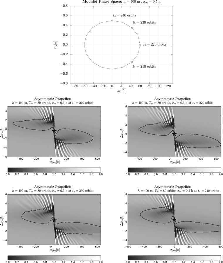
Figure 2. Evolution of the propeller asymmetry for half of a moonlet period. Top panel: phase space representation of the moonlet libration highlighting the four different libration phase angles shown in the center and bottom panels. The moonlet of a size of h = 400 m librates with a period of Tm = 80 orbits and an amplitude of xm,0 = 0.5 h. The snapshots (center and bottom panels) show the moonlet (star symbol) at different libration phases at times of t1 = 210 orbits (middle left), t2 = 220 orbits (middle right), t3 = 230 orbits (bottom left), and t4 = 240 orbits (bottom right).
Download figure:
Standard image High-resolution imageA more detailed analysis of the gap structures will be presented in the following sections.
3.2. Radial Gap Profile
Figure 2 illustrates the evolution of the asymmetry of a propeller caused by a librating moonlet. The gray level density representations correspond to certain times t = (210, 220, 230, 240) orbits, which represent four different phases (phase angles) of the moonlet libration.
We will analyze and compare the radial gap profiles of a symmetric and asymmetric propeller at different azimuthal distances to the moonlet, which demonstrate the changes in the gap structures due to the moonlet motion. The minimum of the surface mass density defines the gap depth and its radial position gives the gap position. At the fixed surface mass density level Σ/Σ0 = 0.8 we estimate the gap width, permitting the comparison of the inner and outer gap in this way.
First, we reduce the noise of the simulation data—especially in the wake region close to the moonlet—by performing moving box averaging for the radial gap profiles, where the radial box length is set close to the wake wavelength of about Δx = 0.5 h. The resulting smoothed radial density profiles of the inner and outer gap at azimuthal distances to the moonlet of  = 10,200 and 600 h are shown in Figure 3. Note that for the bottom panels in Figure 3 we use a moonlet-centered coordinate system (Δx = x−xm(t) and Δy = y−ym(t)) where we subtract of the moonlet's actual position for better comparison to the unperturbed moonlet profiles. The solid and dashed curves denote the inner and outer gap profiles, where we mirrored the inner gap's profile at the origin to compare both gap profiles in a better way.
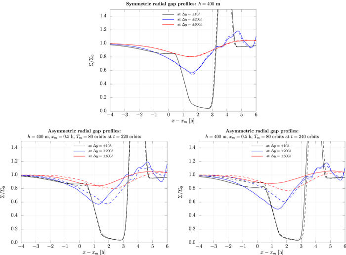
Figure 3. Radial gap profiles for a symmetric (Top) and asymmetric propeller structure (Bottom Left and Right) at different azimuthal distances to the moonlet of Δy = ±10 h (black), ±200 h (blue), ±600 h (red). The dashed and solid lines denote the outer and inner gap profile. The inner gap's profile has been mirrored at the moonlet position for better comparison. For the asymmetric propeller (Bottom panels) the radial gap profile is given at two different libration phases of the moonlet. Here, the moonlet size has been set to h = 400 m and the libration period and amplitude have been set to 80 orbits and 0.5 h. For better comparison, the moonlet's current position has been subtracted of in the case of the asymmetric propeller.
Download figure:
Standard image High-resolution imageThe top panel of Figure 3 shows the radial profile for the symmetric propeller. Here, the gap locations of the inner and outer gap match at all azimuthal distances. Further, the gap relaxes azimuthally as theoretically predicted, i.e., the gap depth decreases for increasing azimuthal distance to the moonlet.
In the bottom panels the asymmetric gap profiles are illustrated at the two snapshots T = 220 orbits and T = 240 orbits from Figure 2. Here, the moonlet is presented at its azimuthal (left) and radial (right) libration amplitude. While in the left panel the gap profiles look much alike, but are shifted radially with increasing azimuth, their depths and widths differ significantly in the right panel. Note how the beginning of the gaps (compare Δy = 10 h) stays unaffected by the moonlet libration and follows the moonlet motion instantaneously in both panels.
3.2.1. Gap Positions
The changes in the gap minima locations caused by the moonlet libration can be better illustrated by considering their time evolution for a fixed azimuth, as shown in Figure 4, where the evolution of the gap minima locations at  = 10,200 and 600 h is presented.

Figure 4. Evolution of the radial gap minima location for the symmetric (left) and asymmetric (right) propeller at azimuthal distances to the moonlet of Δy = ±10 h (black), ±200 h (blue) and ±600 h (red). The coordinate system is moonlet-centered Δx = x−xm(t) and Δy = y−ym(t), meaning that the current moonlet position has been subtracted. The dashed and solid lines denote the outer and inner gap profile. The moonlet's radial position in the right panel is shown by the black dotted line. An increasing radial amplitude of the changing gap minima locations can be seen for larger azimuths. For the simulation the moonlet has the Hill radius h = 400 m and was librating with a period and amplitude of 80 orbits and 0.5 h.
Download figure:
Standard image High-resolution imageFor the symmetric propeller the radial gap positions for different azimuths lay on top of each other, where the mean radial gap position  (at Δy = ±10 h) decreases to
  xgap
xgap ≈ 1.6 h (for Δy = ±200 and ±600 h) for larger azimuthal distances.
Figure 4 shows the time evolution of the gap minima location for the symmetric (left panel) and the asymmetric (right panel) propeller. For the asymmetric case, the moonlet libration (black dotted line) is well reflected by the gap minima locations. Further, the radial amplitude of the gap location slightly increases for larger azimuthal distance to the moonlet. For the symmetric case, the radial gap locations stay constant over time.
While the ring material in the close vicinity to the moonlet almost immediately feels the change in the moonlet's motion (compare the the black solid and dashed lines in Figure 4), the perturbation by the motion of the moonlet first needs to be transported through the ring environment to larger azimuthal distances set by the Kepler shear (see Equation (14)). Thus, when the moonlet reaches its radial libration amplitude of 0.5 h at T = 80 orbits the gap minima at Δy = 200 h and Δy = 600 h are following the moonlet motion after about 26 orbits and 80 orbits, respectively. This agrees with the delay found in Figure 4.
3.2.2. Radial Gap Separation
Although the radial locations of the gap minima change over time and can differ by more than 1 h (compare the solid and dashed red lines in Figure 4), their separation stays almost constant over time (see Figure 5). The evolution of the radial gap separation is presented at azimuthal distances to the moonlet of  = 10, 200 and 600 h, where the dashed and solid lines denote the symmetric and asymmetric gap separation, respectively. With increasing azimuth the scattering of the radial gap separation becomes larger (about 1 h at Δy = ±600 h and 0.5 h at Δy = ±200 h). This is illustrated in the left panel of Figure 5, where a comparison of the gap separation for the symmetric propeller structure (red solid line) along the azimuth is compared against the asymmetric one (black lines) for three different snapshots. Comparing all the curves, one recognizes that up to a critical azimuth of about 250 h the variations of the radial gap separation for the asymmetric gaps are negligible and, thus, it almost matches the symmetric gap structure.
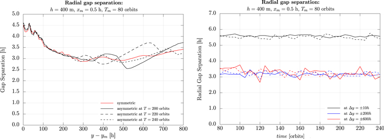
Figure 5. Gap separation for a symmetric and asymmetric propeller structure for a moonlet with h = 400 h Hill radius. For the asymmetric propeller structure the moonlet was librating with a period of 80 orbits and an amplitude of 0.5 h. For all realizations, a moonlet-centered reference frame has been used. Left: radial gap separation along the azimuth. Red and black solid lines denote the symmetric and asymmetric propeller structure. The asymmetric propeller structure is presented at different snapshots at T = 200, 220 and 240 orbits. Right: radial gap separation for a symmetric (dashed) and asymmetric (solid) propeller structure at azimuthal distances to the moonlet of Δy = ±10 h (black), Δy = ±200 h (blue) and Δy = ±600 h (red).
Download figure:
Standard image High-resolution imageFor larger azimuthal distances to the moonlet, the retardation effect gets more dominant resulting in larger variations of the radial gap separation along the azimuth with time. This allows us to detect the perturbation by the moonlet motion, which gets visible as a wavy structure along the azimuth. Further, comparing the different snapshots at times T = 200 orbits and T = 220 orbits the propagation of the perturbation along the azimuth can be observed. On average, the gap separation still follows the azimuthal behavior of the unperturbed gap separation.
3.2.3. Gap Width
The gray level density plots in Figure 1 and the radial profiles presented in Figure 3 demonstrated that the gap width is influenced by the motion of the moonlet. We study the effect of the moonlet motion on the gap width by estimating the gap width at an 80% gap closing (Σ/Σ0 = 0.8).
The resulting gap widths for the inner and outer gap are shown in Figure 6. A concave decrease for all curves can be seen, resulting from the azimuthal gap relaxation. A similar trend holds for the gap depths.

Figure 6. Comparison of the gap width at Σ/Σ0 = 0.8 for the symmetric (dashed) and asymmetric propeller (solid) at T = 220 orbits (left) and T = 240 orbits (right). The widths of the inner and outer gap are given by the black and red colored lines. The results have been obtained from simulations of a h = 400 m sized moonlet, which was librating with a radial amplitude and a period of 0.5 h and 80 orbits for the asymmetric case.
Download figure:
Standard image High-resolution imageIn the panels of Figure 6, the dashed lines refer to the symmetric propeller structure, whereas the solid lines represent the widths of the asymmetric gap structures. The red and black colors denote the outer and inner gap structure. In all representations, the gap widths of the symmetric and asymmetric gaps differ significantly. The moonlet libration can be identified by the intersection points of the inner and outer gap width profiles (right panel, Figure 6), where the gap widths exchange their roles.
Figure 7 shows a comparison of the time evolution of the asymmetric, Wa, and symmetric, Ws, gap widths at two fixed azimuthal distances (Δy = ±200 h and Δy = ±400 h) and for the density level of Σ/Σ0 = 0.8. The left panel shows the evolution of Ws(t) for the symmetric propeller, while the right one shows Wa(t) for the asymmetric propeller. For the symmetric case, the values of Ws for the inner and outer gap fall on to of each other, while they increase in time to reach the saturation steady states, which are  Ws
Ws ≈ 2.7 h for
  and
and  Ws
Ws ≈ 1.9 h for
  . The latter lower value is to be expected because the viscous diffusion reduces the width Ws/a(Δy) with a growing azimuth, Δy.
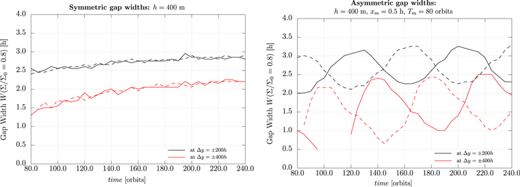
Figure 7. Comparison of the gap width evolution of the inner (solid) and outer (dashed) propeller gap for a non-librating (left) and librating (right) central moonlet at Σ/Σ0 = 0.8 for  (black) and Δy = ± 400 h (red). For the non-librating moonlet, the values of Ws(t) fall on top of each other, giving mean values of
  Ws
Ws ≈ 2.7 h for Δy = ±200 h and
  Ws
Ws ≈ 1.9 h for Δy = ± 400 h, respectively. For the librating moonlet, the gap widths oscillate with the moonlet and show an anti-phase relation. Their mean values slightly differ:
  Wa(Δy = ±200 h)
 = 2.76 h against
  Wa(Δy = ±400 h)
 = 1.8 h for the inner gap and
  Wa(Δy = ±200 h)
 = 2.63 h against
  Wa(Δy = ±400 h)
 = 1.56 h for the outer gap. Interestingly, the amplitude of the oscillation increases for a larger azimuth.
Download figure:
Standard image High-resolution imageThe case for the librating moonlet is quite different, given in the right panel of Figure 7, where the widths, Wa(t), oscillate with the libration of the moonlet and are obviously in opposite phases (anti-phase). Again, the mean values,  Wa
Wa , are smaller for the larger azimuthal cut at Δy = ±400 h, while, interestingly, the amplitude of the oscillation is larger (about
  Wa(Δy = ±200 h)
 = 2.76 h against
  Wa(Δy = ±400 h)
 = 1.8 h for the inner gap and
  Wa(Δy = ±200 h)
 = 2.63 h against
  Wa(Δy = ±400 h)
 = 1.56 h for the outer gap).
3.2.4. Gap Depth
Another measurable quantity is the gap depth, given by  . As in the asymmetric case, the gap widths, W(t), and lengths, L(t), are changing with time, which is an analogous behavior to be expected for d(t).
Figure 8 shows the time evolution of d(t) for the symmetric case (left panel) and the asymmetric case (right panel) for different values of Δy.
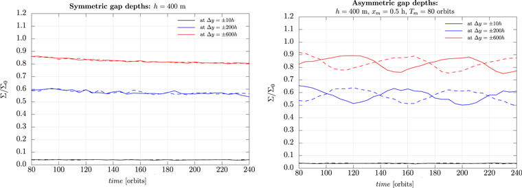
Figure 8. Evolution of the propeller gap depth for the symmetric (left) and asymmetric (right) propeller at different azimuthal positions to the moonlet Δy = ±10 h (black), Δy = ±200 h (blue), and Δy = ±600 h (red). The solid and dashed lines represent the inner and outer propeller gap.
Download figure:
Standard image High-resolution imageWhile for the symmetric case (left panel), the values of ds(t) for the outer and inner propeller wing coincide and slightly relax to the steady state, the asymmetric value of da(t) (right panel) oscillates with the moonlet libration, which is similar to the width, Wa(t). The amplitude of this depth-variation is about  .
.
3.3. Azimuthal Gap Relaxation
To estimate the azimuthal gap relaxation, we study the dependence of the gap minimum on the azimuthal distance to the moonlet.
In order to extract the azimuthal gap profiles, we smooth the radial profiles with a moving box averaging method, where the box size has been set to Δx = ±0.5 h. This reduces the radial scattering of the gap minima locations especially in the wake region. Further, we use another moving box averaging process to avoid the azimuthal scattering of data due to the wakes. For this reason, we set the box size to Δy = ±25 h. The resulting azimuthal gap relaxation profiles are shown in Figure 9 for the symmetric (dashed lines) and asymmetric (solid lines) propeller.
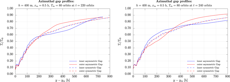
Figure 9. Azimuthal gap relaxation profile for the symmetric (dashed) and asymmetric (solid) gap structure at T = 220 orbits (left) and T = 240 orbits. Comparing the inner (blue) and outer (red) gap profiles in the symmetric case, we clearly see how both profiles match perfectly. In the asymmetric case, the symmetry of the propeller is broken, which can be seen from the different lengths and the different depths of the gaps at different azimuthal distances to the moonlet.
Download figure:
Standard image High-resolution imageIn the left and right panels, the asymmetric propeller minima are presented at orbit 220 and 240 of the integration time, respectively. The red and blue colors denote the outer and inner gaps. By comparing the non-librating and librating moonlet, a clear difference in the gap relaxation can be observed. While the symmetric propeller the inner and outer gap is closing in the same way with growing azimuth (except small variations due to the wakes and noise), the gap depths change along the azimuth for the asymmetric propeller.
Due to the retardation, the influence of the changes in the moonlet's radial libration are found by the intersection points of the minima density curves (see right panel of Figure 9) for the inner and outer gap. As an example, as seen in the right panel, the inner gap closes faster than the outer gap until an azimuthal distance of 400 h to the moonlet. There, an intersection point of both gap profile curves can be found. From this distance on, the outer gap closes faster and stays over the density minima of the inner gap. This intersection point is caused at T ≈ 200 orbits, where the moonlet is at its lowest radial elongation, xm = −0.5 h (compared with Figure 4). At this turning point, the moonlet starts to migrate outward again.
3.3.1. Gap Length
From the azimuthal gap profile, we define the gap length, L80, as the azimuthal distance to the moonlet at Σ/Σ0 = 0.8 for the inner and outer gap structure.
The evolution of the gap length L80(t) = L(Σ/Σ0 = 0.8, t) is presented in Figure 10, where the symmetric (red color) and asymmetric (black color) propellers are presented. The dashed and solid lines denote the outer and inner gaps. The dotted line represents the azimuthal evolution of the azimuthal moonlet position as a reference. The asymmetric propeller gap length varies in phase with the moonlet motion. For the non-librating central moonlet, the mean gap length,  L80
L80 , is about 539.5 h, while the for asymmetric propeller, the mean gap lengths slightly differ (
 L80
L80 = 511 h for the inner gap against
  L80
L80 = 523 h for the outer gap) and the maximum difference of the gap lengths is about 300 h, respectively.
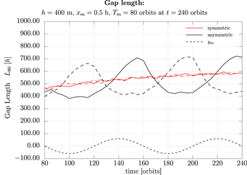
Figure 10. Comparison of the gap length at a 80% relaxation for the symmetric (red) and asymmetric propeller (black). The length of the inner and outer gap are given by the solid and dashed lines. The results have been obtained from the simulation of a h = 400 m sized moonlet. For the asymmetric propeller, the moonlet was librating with a radial amplitude of 0.5 h and a period of 80 orbits. For comparison, the azimuthal evolution of the librating moonlet is plotted as the black dotted line as well. For both profile plots, a moonlet-centered reference frame has been chosen for a better comparison.
Download figure:
Standard image High-resolution imageAlthough the depths of the gaps only differ by about 10% (compared in Section 3.2.4), these variations result in large azimuthal changes in the gap lengths. Thus, studying the azimuthal gap profiles is the favorable method to search for the imprint of the asymmetry.
3.4. The Gap Contrast
As already carried out, the azimuthal gap profiles of the inner and outer gap structures differ for a librating moonlet. In order to extract the perturbation by the moonlet motion and to study its propagation through the gaps, we define the gap contrast as the difference of the inner and outer gap profiles.
The retardation of the symmetry-breaking perturbation by the moonlet libration along the gap length sets a memory timescale, Tgap. Changes in the radial moonlet motion, which happen within this timescale, become visible as zero value crossings and help to distinguish a periodic motion from a migration in this way.
Figure 11 shows the gap contrast estimated from the azimuthal gap relaxation profiles presented in Figure 9. The red solid line represents the gap contrast of the symmetric propeller structure along increasing azimuthal distance to the moonlet. Its maximum corresponds to deviations caused by the wake region (Σ/Σ0 ≈ 2 × 10⁻²) and, thus, defines the level where the symmetric and asymmetric propeller will not be distinguishable anymore. The black lines in Figure 11 represent the gap contrast for the asymmetric gap structure at different integration times, where the solid, dashed, and dotted lines show the gap contrast at T = 200, 220, and 240 orbits. The different snapshots for the asymmetric propeller demonstrate how the perturbation by the moonlet libration propagates through the gaps. As an example, the minimum at T = 200 orbits shifts from Δy = 200 h and Σ/Σ0 = −0.1 to Δy = 400 h and Σ/Σ0 = −0.12 at orbit 220 and further to Δy = 650 h and Σ/Σ0 = −0.1 at orbit 240. The transport of perturbations along the azimuth resembles a propagating wave package. Like a dissipating wave package, the perturbation gets smeared along the azimuth due to diffusive effects.

Figure 11. Difference of the azimuthal gap relaxation of the inner and outer gap (gap contrast) for a non-librating (red) and librating (black) central moonlets of the size of h = 400 m at orbits 200, 220, and 240 (solid, dashed, and dotted lines).
Download figure:
Standard image High-resolution image4. Ring–Moonlet Interactions
The symmetry breaking of the propeller structure disturbs the force balance of the gravity by the ring ensemble reacting on the moonlet (Seiler et al. 2017). Here, we calculate the resulting force of the surrounding ring material on the moonlet. Therefore, we calculate the gravity of every grid cell onto the moonlet and sum over all the contributing cells of the grid. We exclude a circular area of ![$r={\left[{\left(x-{x}_{m}\right)}^{2}+{\left(y-{y}_{m}\right)}^{2}\right]}^{1/2}\,=1.2\,{\rm{h}}$](https://content.cld.iop.org/journals/0067-0049/243/2/31/revision1/apjsab26b0ieqn58.gif) around the moonlet from the force calculation in order to account for the physical dimension of the moonlet, which is treated as a point mass in our simulations.3
The resulting total gravitational interaction between the ring and the moonlet, Fx and Fy, in the radial and azimuthal direction is given by the sum of the contributing cells:
around the moonlet from the force calculation in order to account for the physical dimension of the moonlet, which is treated as a point mass in our simulations.3
The resulting total gravitational interaction between the ring and the moonlet, Fx and Fy, in the radial and azimuthal direction is given by the sum of the contributing cells:


with  i = (xi, yi) and
  m = (xm, ym) as the position vectors of the ith cell and the moonlet. Here, ΔA = Δxi × Δyi denotes the surface area of the individual equal-sized grid cells, and ΔΣi = Σi − Σ0 denotes the difference of the current and unperturbed surface mass density.4
The left panel in Figure 12 illustrates the evolution of the normalized ring gravity, where the x (red) and y (blue) component of the ring gravity follow the moonlet motion (xm and ym are represented by the dashed and solid black lines). The right panel shows a comparison of the gap contrast evolution and the moonlet evolution, where the gap contrast is presented at three different azimuthal distances to the moonlet. The evolution for Δy = ±200 h and δy = ±600 h displays the retardation set by the Kepler shear and the decreasing amplitude of the gap contrast with increasing azimuths. While the force has a fixed offset to the moonlet motion (the x component almost falls on top of the radial motion of the moonlet, whereas for the y component of the ring force has an offset of about 50 orbits or 90°), an increasing phase shift in the gap contrast for larger azimuths can be found, which are caused by the retardation.
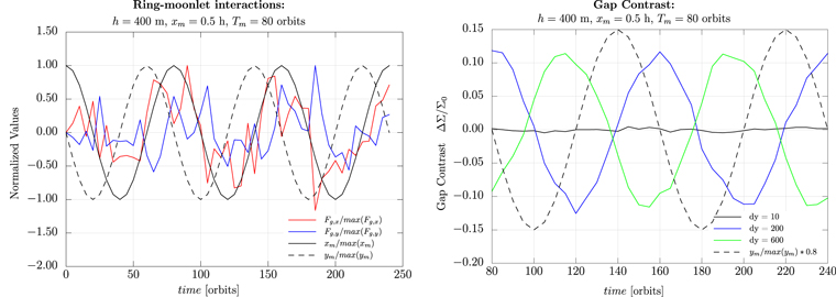
Figure 12. Left: time evolution of the normalized moonlet motion in x (black dashed line) and y (black solid line) direction and the x (blue) and y (red) component of the ring gravity acting on the moonlet. Right: evolution of the gap contrast at different azimuthal positions, illustrating how the variation of the gap contrast follows the moonlet motion (black dashed line).
Download figure:
Standard image High-resolution image5. Systematic Asymmetry Predictions
In this section, we test the dependence of the propeller's asymmetry on (a) the libration amplitude and (b) the libration period. This allows us to make predictions for the observability of the asymmetry of propeller gap structures in Saturn's rings. Therefore, at first, we keep the libration period constant at Tm = 80 orbits and vary the initial radial amplitude, xm,0. In a second analysis, we perform simulations where the initial radial amplitude of xm,0 = 1 h will be kept constant, while the libration period is varied. For both scenarios, we will study the gap contrast, the gap length, and the width at Σ/Σ0 = 0.8. Note that due to the modeled moonlet motion given by Equation (12), the azimuthal amplitude is also affected in both scenarios.
Note that our analysis does not consider any resonances in the vicinity of the propeller structure, which might have an additional effect of the final asymmetry for larger radial amplitudes and libration periods.
For each simulation parameter at each time, the above quantities will be determined. Further, the mean value, the maximum, and the minimum at each time will be estimated as a function of the azimuth. Finally, for the complete simulation time frame, the global maximum, the minimum, and the mean values will be calculated. The resulting values will be presented in the following sections.
5.1. Dependence of Asymmetry on the Libration Amplitude
We vary the libration amplitude, xm,0, from 0.125 h through 4 h.
In Figure 13, the dependence of the maximum gap contrast on the radial amplitude of the moonlet libration is shown. Here, we can fit the data by the exponential relation,

with Ci,0 = 0.925, Ci,1 = 0.971, and λi = 0.458 h−1 for the maximum gap contrast and Co,0 = 0.923, Co,1 = 0.974, and λo = 0.458 h−1 for the minimum gap contrast.

Figure 13. Dependence of the maximal asymmetry from the moonlet's libration amplitude for constant libration period of Tm = 80 orbits.
Download figure:
Standard image High-resolution imageStarting from small amplitudes, the contrast increases for the growing initial amplitude until a saturation of about C = 0.925 is reached. A further increase of the libration amplitude does not affect the gap contrast. For amplitudes xm,0 > 1.6 h, a steady state for the propeller structure cannot be reached anymore due to the strong perturbation by the moonlet motion. Thus, only the gap area close to the moonlet, where the retardation is small enough forms and survives the moonlet motion, which explains the maximum saturation level.
Figure 14 illustrates the dependence of the gap length, L80, (left panel) and the gap width, Wa, (right panel) on the libration amplitude. For the gap length, a clear drop in the mean gap length can be noticed for larger amplitudes, while the difference between the maximum and minimum gap lengths of the inner and outer gap first increases from 200 h to 500 h for xm,0 = 0.125 h to xm,0 = 1 h and then reduces to about 200 h. The gap width changes as well with the gap length (see right panel of Figure 14), but here, the mean gap width increases from 2.25 h to 2.6 h for larger amplitudes, until about xm,0 = 1.6 h when a saturation level is reached. A similar result can be seen for the difference between the maximum and minimum gap widths of the inner and outer gap, which increases from 0.5 h to 3.5 h, respectively.
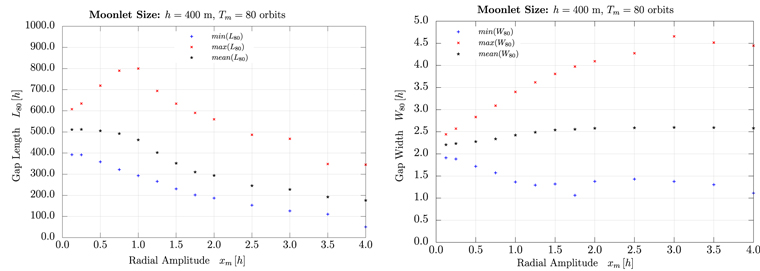
Figure 14. Dependence of the maximum, minimum, and mean gap length (left) and gap width (right) at Σ/Σ0 = 0.8 on the moonlet's libration amplitude. These values refer to measurements for the inner and outer gap.
Download figure:
Standard image High-resolution imageTo summarize, with larger radial amplitudes, the perturbation by the moonlet motion increases, which results in shorter gap lengths, broader gaps, and larger gap contrast until the perturbation exceeds a critical level, where the creation of the propeller structure is prevented.
5.2. Dependence of Asymmetry on the Libration Period
We vary the libration period of the moonlet from Tm = 15 orbits to Tm = 320 orbits, while we keep the radial amplitude fixed at xm,0 = 1 h.
Figure 15 shows the dependence of the gap contrast on the libration period, where an exponential relation given by

where C0 = 0.125, C1 = 0.587, and λ = 0.013 orbit−1 can be found.

Figure 15. Dependence of the maximal asymmetry on the moonlet's libration period for a constant radial amplitude of xm,0 = 1 h.
Download figure:
Standard image High-resolution imageFor a fixed radial amplitude, the changes for larger libration periods result in a growing azimuthal excursion of the moonlet (see Equation (12)). As the libration period grows, the relative velocity to the unperturbed orbit decreases and, thus, the perturbation by the changing moonlet position can be easily transported to larger azimuthal distances, resulting in a more symmetric propeller structure and, therefore, in a lower gap contrast (see Figure 15).
In Figure 16, the dependence of the gap length (left panel) and the gap width (right panel) on the libration period is presented.

Figure 16. Dependence of the gap length (left) and gap width (right) at a 80% gap relaxation on the moonlet's libration amplitude for a fixed radial amplitude of xm,0 = 1 h.
Download figure:
Standard image High-resolution image
The gap length (left panel) first increases from 350 h to about 500 h with respect to the libration period interval from T0 = 15 orbits through T0 = 80 orbits. For this interval, the difference between the maximum and minimum gap lengths of the outer and inner gap increase from 400 h to about 600 h. At Tm = 80 orbits, the gap passage time equals the libration period of the moonlet, allowing the perfect transport of the perturbation through the gaps. At this optimal parameter set, the gap width reaches its maximum of about 2.5 h, respectively, while the differences between the maximum and minimum gap widths of the inner and outer gap are at their maximum of about 2 h (compare with the right panel). For increasing libration periods, the relative velocity of the moonlet to its unperturbed orbit decreases, resulting in smaller perturbations and, therefore, in a more symmetric propeller structure. For this reason, the mean gap length drops to about 500 h—close to the value of the unperturbed propeller gap length. Further, the differences between the maximum and minimum gap lengths drops to an almost constant level of 200 h as well. By exceeding a libration period of Tm = 80 orbits, the mean gap width stays almost constant at 2.5 h, which is very close to the unperturbed value of 2.6 h. Nevertheless, the moonlet motion still induces a difference of the gap widths of about 1 h.
To summarize, for small libration periods (Tm ≤ Tgap), the asymmetry is large because of the strong perturbation by the moonlet motion and the retardation, while for large periods (Tm > Tgap), the asymmetry gets smaller due to quasi-static changes in the moonlet motion. However, the asymmetry is still measurable but depends on the actual libration phase angle of the moonlet at the observation time.
5.3. Application to the Propeller Blériot
The excess motion of Blériot has been reconstructed by three overlaying harmonic functions. In the following, we assume the moonlet to librate with the largest amplitude of about max(ym) = 1845 km and with a libration period of 11.1 yr (see e.g., Seiler et al. 2017; Spahn et al. 2018). Translating the fitted period to the number of orbits results in Tm = 11.1 yr = 6941 orbits and, thus, the radial amplitude for the moonlet (see Equation (13)) is given by

This agrees with the radial amplitude estimated from orbital fits by Spahn et al. (2018), who estimated the radial deviation to be about 200 m. The Hill radius of Blériot is about h = 400 m (Hoffmann et al. 2016; Seiler et al. 2017) and, thus, the estimated radial amplitude corresponds to xm,0 ≈ 0.4 h.
For Blériot, Seiler et al. (2017) estimated Tgap ≈ 0.5 yr, which corresponds to 313 orbits, respectively. Thus, for Blériot, we need to consider the case of Tm = 11.1 yr = 6941 orbits ≫313 orbits = 0.5 yr = Tgap. At this ratio, the gap contrast is already at its lowest level of about 0.125 in comparison to the noise level of the unperturbed propeller gap contrast of 0.02.
The maximum gap contrast illustrated in Figure 13 can be linearly approximated in the range of xm,0 = [0, 1.5 h]. Therefore, the expected gap contrast level of about C0 = 0.125 estimated for xm,0 = 1 h (see Figure 15) can be interpolated to xm,0 = 0.5 h, yielding 0.063, respectively. Following this interpolation, the maximum variation in gap length and gap width are expected to be about 125 h and 0.5 h, respectively.
6. Conclusion and Discussion
In this work, we studied the formation of asymmetric propeller structures in Saturn's A ring, assuming a libration of the moonlet. We considered the libration of the moonlet as given. Instead of calculating the eigenfrequency of the propeller–moonlet oscillator, as suggested by Seiler et al. (2017), we treated the moonlet's libration period and amplitude as variables, which allowed us to study the dependence of the asymmetry on these parameters in more detail. Further, we studied the dependence of the asymmetry on the libration parameters (the amplitude and period). In practice, the librational behavior sensitively depends on the perturbation forces and sources (e.g., resonances, density fluctuations, and particle collisions). It turned out that the additional moonlet motion is perturbing the induced propeller structure, causing an asymmetry in this way. The perturbation by the moonlet motion gets transported through the gaps with the Kepler speed and, thus, arrives at the gap ends after a delay time, Tgap. This retardation depends on the gap length and sets a memory time, which finally causes the asymmetric appearance of the propeller structure in the images. The main implications of our simulations are as follows.
6.1. Timescales versus Asymmetry
We studied the dependence of the asymmetry on the libration period (see Figures 15 and 16). Three general cases were investigated:
- (i)Tm < Tgap. For small libration periods the asymmetry is large. This results from the strong perturbation by the moonlet motion that causes large variations in all gap properties, which even can prevent the propeller formation. Thus, small libration periods are similar to the scenario of large libration amplitudes.
- (ii)Tm = Tgap. The strongest asymmetry has been identified if the libration period matches the gap timescale. In this case, the perturbation by the moonlet motion gets transported in the most effective way (in a synchronized way), resulting in the largest variations in the gap length and width.
- (iii)Tm > Tgap. The quasi-static changes in the moonlet motion result in a less asymmetric shape of the propeller. Thus, the gap contrast is minimal and the variations in the gap width and gap length are rather small, which we found to be the case for Blériot.
6.2. Libration versus Migration
The retardation limits the observability of the asymmetry and with it the chance to distinguish a migration of the moonlet from a libration. Changes in the direction of the moonlet motion (inward and outward movement) result in zero value crossings in the gap contrast along the azimuth (see Figure 11). Depending on the libration period, three limiting cases can be distinguished:
- (i)Tm < Tgap. The frequent changes in the moonlet motion can be seen due to the retardation, resulting in, at minimum, two intersection points in the gap profile (or zero values crossings for the gap contrast, respectively). Thus, the periodicity of the moonlet motion is well reflected by the propeller.
- (ii)Tm = Tgap. At maximum, two (at minimum, one) intersection points in the azimuthal gap profile can be identified, depending on the libration phase of the moonlet at the observation time.
- (iii)Tm > Tgap. The slow outward and inward migration of the moonlet results in, at maximum, one (at minimum, zero) observable intersection points.
In order to identify a librational motion of the moonlet, the libration period needs to be smaller than the memory time, Tm < Tgap. For larger libration periods, the gap contrast will only change its sign at the turning points of the radial moonlet libration. In between, no change in its sign will be visible and, therefore, the moonlet libration might be misinterpreted as a radial drift.
6.3. Observability of the Asymmetry
In order to measure the asymmetry of the propeller structure, our analysis has shown that the azimuthal profiles are the most favorable to consider for processing Cassini ISS images (see Figure 9). In those profiles, small differences in the gap depth (Σ/Σ0) for the inner and outer gap can result in large differences in the gap lengths (compared with Figure 10).
However, in cases of high-resolution observations, such as stellar occultations by Cassini's Ultraviolet Imaging Spectrometer (UVIS), small variations in the radial gap profile can be resolved, allowing us to study the asymmetry even in those profiles.
Nevertheless, in all cases, both the inner and outer gap need to be recorded.
6.4. Asymmetry of the Propeller Blériot
Our predictions show that the asymmetry in the gap contrast should be about 6.3%, which is still larger than the noise level for the unperturbed propeller. The gap width differences comparing inner and outer gap structure should be about 0.5 h, and the gap lengths are expected to differ by 125 h. These variations should be still detectable but depend on the libration phase of the central moonlet at the time of observation.
Due to the large libration period of Blériot, at maximum, one zero value crossing for the gap contrast can be expected, which makes it impossible to judge whether the moonlet is librating or migrating considering one single observation. An analysis of several images of Blériot at different times would be necessary to search for moving patterns (changes in the sign and amplitudes) in the gap contrast along the azimuthal direction.
6.5. Asymmetry of Other Propellers
Although the asymmetry for Blériot might be rather small, the asymmetry for the other giant trans-Encke propellers might be easier to detect. Moonlets smaller than Blériot have smaller inertia and, thus, suffer more from moonlet–ring interactions (e.g., collisions), resulting in larger radial variations and, thus, in larger asymmetries (see Figure 13). As an example, the propeller structure Earhart is smaller than Blériot (h ≲ 300 m) but shows a similar amplitude in its longitude residual for a shorter observational period (Spahn et al. 2018), resulting in a larger radial amplitude for an assumed moonlet libration (xm ≳ 1.5 h from Equation (13)). For this expected amplitude, an asymmetry should be observable, even for libration periods of Tm ≫ Tgap. Further, due to the smaller size of these moonlets, their induced propeller wings' azimuthal extents are smaller by Mm/ν0 ∝ h3/ν0 ∝ L (Spahn & Sremčević 2000; Sremčević et al. 2002) and, thus, allow us to record both propeller wings at the same time with one observation. This would give us the chance to reconstruct the evolution of the perturbation by the moonlet motion through the gap structures.
6.6. Propeller–Moonlet Interactions
The formation of an asymmetric propeller structure due to the motion of the moonlet causes an unbalanced force of the ring material on the moonlet (see Figure 12). Calculating the force of the ring material on the moonlet, we find that it is dominated by the azimuthal amplitude of the moonlet (Seiler et al. 2017) and follows the moonlet motion with a phase shift according to the Kepler shear. Thus, our simulations agree with the simple propeller–moonlet interaction model suggested by Seiler et al. (2017).
6.7. Outlook
Although the implementation of a librating moonlet is a simplification, our simulation, however, gives an insight into how the propeller structure reacts to perturbations and what the resulting asymmetry will look like. Further, our simulations have shown that the retardation along the azimuth is the main mechanism to make the asymmetry measurable in the images. Therefore, even for an underlying stochastic migration of the central moonlet, an asymmetry of the induced propeller structure might form. The observability of the resulting asymmetry then will depend on the collision frequency and the memory time of the gap.
However, in order to build a fully consistent model, as a next step, the moonlet needs to be simulated in a box where it is allowed to move freely. In this way, a stochastic moonlet motion can be simulated as well, which can be directly compared to the unperturbed and librating moonlet.
Further, allowing the moonlet to move freely within the simulation box will show whether the back-reaction of the ring material is able to conserve an initial libration of the moonlet, which will be the final consistency test for the suggested propeller–moonlet interaction model.
Our introduction of the gap contrast allows us to directly observe the azimuthal propagation of the perturbation by the moonlet motion (see Figure 11). We found that, for a librating moonlet, the perturbation propagates through the gap structures similar to a moving wave package that propagates through a dissipative medium. An analysis of the azimuthal gap profiles for the known wandering trans-Encke propellers would allow us to calculate the gap contrast and to seek for a possible moonlet motion inducing asymmetry.
Our simulation code uses an isothermal model for the ring environment. This might result in larger viscosity values in the close vicinity of the moonlet. For a consistent model, the temperature needs to be considered in the simulations as well by including the energy equation. This might have an additional effect on the observability of the asymmetry.
This work has been supported by the Deutsche Forschungsgemeinschaft (Sp 384/28-1,2 and Ho 5720/1-1) and the Deutsches Zentrum für Luft-und Raumfahrt (OH 1401). We thank the referee P. D. Nicholson for carefully reading our article and for his helpful comments.
Footnotes
- 1
In these simulations, a test moonlet, which has been placed on the expected orbital position of Blériot, has been driven gravitationally by Saturn and 15 of its larger moons.
- 2
Including the oblateness of Saturn induces slightly different orbital frequencies of Ω, ν, and κ, resulting in a precession of the ascending node and the pericenter. This precession affects all ring material within the simulation area, including the moonlet. Thus, a modified mean motion would be necessary for the corotating frame. Within the corotating simulation box, the effective differences would be still present but rather small (about 1%), as discussed by Seiß et al. (2019).
- 3
We choose a value of r = 1.2 h to consider a moonlet, which completely fills its Hill sphere plus a little threshold. However, varying r mainly changes the amplitude of the resulting force, while the phase shift to the moonlet motion remains.
- 4
Considering ΔΣi instead of Σi omits convergence problems at the edges of the simulation grid.