


Abstract
The radial velocity (RV) method plays a major role in the discovery of nearby exoplanets. To efficiently find planet candidates from the data obtained in high-precision RV surveys, we apply a signal diagnostic framework to detect RV signals that are statistically significant, consistent in time, robust in the choice of noise models, and do not correlated with stellar activity. Based on the application of this approach to the survey data of the Planet Finder Spectrograph, we report 15 planet candidates located in 14 stellar systems. We find that the orbits of the planet candidates around HD 210193, 103949, 8326, and 71135 are consistent with temperate zones around these stars (where liquid water could exist on the surface). With periods of 7.76 and 15.14 days, respectively, the planet candidates around star HIP 54373 form a 1:2 resonance system. These discoveries demonstrate the feasibility of automated detection of exoplanets from large RV surveys, which may provide a complete sample of nearby Earth analogs.
Export citation and abstract BibTeX RIS
1. Introduction
One of the ultimate goals of exoplanet research is to find nearby Earth-like planets. The radial velocity (RV) and transit methods have made the main contributions to exoplanet detections. RV measurements for nearby bright stars can be made relatively efficiently and have enabled planets to be discovered around a significant fraction of them. The transit technique is relatively more sensitive to faint and distant stars. Considering the rare occurrence rate of transit events, the RV method is still of great importance for discovering nearby planets, as evidenced by the detection of Proxima Centauri b (Anglada-Escudé et al. 2016), although the Transiting Exoplanet Survey Satellite is poised to find thousands of nearby transit systems (e.g., Ricker et al. 2014).
Since the Earth is the only planet known to host life, a conservative path to the detection of extraterrestrial biosignatures is to find an Earth-like planet around a Sun-like star (also called an "Earth twin"). To detect such signals, we need to have high-precision RV data that is sensitive to about 0.1 m s−1 RV variations (Mayor et al. 2014). For less massive stars like M dwarfs, the signals corresponding to Earth-sized planets in their temperate zones (where liquid water can exist on the surface; Kopparapu et al. 2014) can be as high as 1 m s−1. To distinguish from the Earth twins, we call these planets "Earth analogs." Thanks to the recent development of high-precision spectrometers, such as Echelle SPectrograph for Rocky Exoplanets and Stable Spectroscopic Observations (ESPRESSO; Pepe et al. 2010) and NN-explore Exoplanet Investigations with Doppler spectroscopy (NEID; Schwab et al. 2016), as well as advanced noise modeling and activity mitigating techniques (Feng et al. 2017b; Dumusque 2018), we are moving toward the detection sensitivity of Earth twins, though multiple issues related to stellar activity and instrumental stability (e.g., Fischer et al. 2016) still need to be resolved.
The availability of long-term, high-precision spectroscopic observations is one of the basic requirements in the discoveries of Earth analogs, such as Proxima Centauri b (Anglada-Escudé et al. 2016), GL 667 Cc (Anglada-Escudé et al. 2013), and Luyten b (Astudillo-Defru et al. 2017). To this end, the Carnegie Planet Finder Spectrograph (PFS; Crane et al. 2010) is one of the major instruments dedicated to performing a high-precision spectroscopic survey of nearby stars. Since its commissioning in 2010, it has made important contributions to the discovery (Proxima Centauri b at 1.3 pc, Anglada-Escudé et al. 2016; Barnard's star b at 1.8 pc, Ribas et al. 2018) and characterization (GJ 9827 bcd at 30 pc, Teske et al. 2018) of nearby planets.
In this work, we use PFS survey data presented in Section 2 and describe how it is processed with a signal diagnostic framework in Section 3 and apply it to the PFS survey data, and then we select signals that are statistically significant, consistent in time, uncorrelated with stellar activity indicators, and robust to the choice of noise models. We then identify planet candidates from these signals and discuss 15 of the most significant signals individually in Section 4. Finally, we conclude in Section 5.
2. Data
The PFS measures the Doppler shift of stellar spectral lines through calibration with the spectrum of iodine (e.g., Marcy & Butler 1992). The calibration and the barycentric correction of the spectrum are implemented through the procedures introduced by Butler et al. (1996). The Ca ii HK (converted to the S-index) and the Hα lines are extracted from the spectrum to assess the stellar activity level. The photon noise is calculated through photon counts by assuming a Poisson distribution. We consider this photon noise to be an indicator of instrumental and/or stellar noise because it can modulate the uncertainty of RV measurements and thus change the likelihood of a periodic signal.
For all PFS targets, we find the relevant astrometry, systematic RV, and luminosity from Gaia data release 2 (DR2; Gaia Collaboration et al. 2018) through crossmatching using a search cone of 2'. The Gaia source corresponding to a PFS target is identified by selecting the brightest star among all matched sources. This approach works because most PFS targets are stars that are bright and have an apparent visual magnitude of less than 15. The mass of a star is estimated through the mass–luminosity functions introduced by Malkov (2007), Eker et al. (2015), and Benedict et al. (2016). The stellar type of each star is found by crossmatching the PFS targets with the Simbad database (Wenger et al. 2000).
3. Initial Selection of Planet Candidates
We define a signal diagnostic framework to identify signals in the PFS RV data. The following steps are used to search and constrain signals.
- 1.We calculate the Bayes factor periodograms (BFPs) for activity indices using Agatha (Feng et al. 2017a) and identify activity signals at periods of Pactivity. In the calculation of BFP, we use the first order moving average model (MA(1); Tuomi et al. 2013) to account for time-correlated noise. Compared with traditional periodograms, such as the Lomb–Scargle periodogram (Lomb 1976; Scargle 1982), the BFP is able to model the excess white noise as well as the red noise in a time series.
- 2.We calculate the BFPs for the RV data using the white, MA(1), and first auto-regressive (AR(1); Tuomi & Anglada-Escudé 2013) noise models and identify signals for each noise model (called "BFP signals" at periods of PBFP). Although AR(1) might lead to false negatives according to Tuomi & Anglada-Escudé (2013), we use it to test whether an RV signal is noise-model dependent.
- 3.We use the adaptive Markov Chain Monte Carlo (MCMC) algorithm (called "DRAM") developed by Haario et al. (2006) for model and parameter inferences. Specifically, we launch tempered (hot) chains to find the global maximum of the posterior and use nontempered (cold) chains to constrain the maximum a posterior (MAP) signal. Such a combination of hot and cold chains allows the parameter space to be well explored without getting stuck in the local maxima. This approach incorporates model complexity by considering prior distributions. Our algorithm is similar to the hybrid MCMC algorithm developed by Gregory (2011). Similar to our previous works (Feng et al. 2017b), we adopt a semi-Gaussian prior distribution with a zero mean and a 0.2 standard deviation for eccentricity to account for the eccentricity distribution found in RV planets (Kipping 2013) and in transit systems (Kane et al. 2012; Van Eylen et al. 2019). Such a broad semi-Gaussian distribution allows solutions with relatively high eccentricity but penalizes solutions with extremely high eccentricity. We adopt uniform priors for the logarithmic orbital period and for other orbital parameters.We constrain each RV signal in the data until any additional signal does not increase the likelihood significantly. In other words, a signal is statistically significant only if its inclusion in the RV model leads to a Bayes factor (BF) of larger than 150 or ln(BF) > 5 (Kass & Raftery 1995; Feng et al. 2016). The BF is the ratio of marginalized likelihoods (or evidences) for two models. We derive the BF from the Bayesian information criterion following Kass & Raftery (1995). Thus, the calculation of the BF in this work assumes uniform prior distributions of model parameters. This BF criterion is found to be optimal compared with other information criteria based on analyses of simulated and real RV data sets (Feng et al. 2016). Therefore, we use the BF criterion to assess the significance of signals.The optimal noise model is chosen according to the model comparison scheme in Agatha (Feng et al. 2017a). According to the comparison of various noise models for both synthetic and real RV data sets (Feng et al. 2016), the MA models are optimal for avoiding false positives and negatives. Hence, we compare the lower and higher order MA models by calculating their BFs. We select the most complex model (with the highest order) that passes the criterion of ln(BF) > 5. For example, we calculate the maximum likelihoods for the white noise, MA(1), MA(2), and MA(3) models for an RV data set. The logarithmic BFs for MA(1) and the white noise model and for MA(2) and MA(1) are larger than five, while the logarithmic BF for MA(3) and MA(2) is less than five. The optimal noise model would be MA(2) because it is complex enough to model the time-correlated noise in the data and is simple enough to avoid overfitting.
- 4.We define a moving time window and calculate the BFP for each step. In other words, we calculate BF(Pi, Wj) (or BFij) for the ith period for the jth time window (Wj) and form a two-dimensional power spectrum. Because the number of RVs in different time windows is different, we normalize BFij for each time window to compare the consistency of signals across time windows. Specifically, we scale the maximum BF for time window Wj to one through
 , where BF = {BF1j, BF2j, BF3j, ...}. To optimize the visualization of the significance of signals as a function of time, the window sizes and steps are chosen according to the sampling and size of the data, as well as the period of target signal. For example, for a set of 100 RVs sampled uniformly over a time span of one year, we can divide the time span into 12 bins and calculate the BFP for the RVs in each bin or time window to investigate the time consistency of signals with orbital periods less than 30 days. For long-period signals, broader time windows should be defined. This example provides a rule of thumb for the choice of window sizes and steps. We call this two-dimensional BFP the "moving periodogram." It is used to check the time consistency of signals identified by MCMC (called "MCMC signals" at periods of PMCMC). We refer the readers to Feng et al. (2017a) for more details.
 - 5.We assess the overall quality of an MCMC signal. A genuine Keplerian (due to a planet) signal should:
- (a)be robust in the choice of noise models. The difference between the period of the MCMC signal and the corresponding BFP signals is less than 10% (i.e., 0.9PBFP < PMCMC < 1.1PBFP).
- (b)not be caused by stellar activity. The difference between the period of the MCMC signal and the signals with the two highest BFs for each activity index is less than 10% (i.e., PMCMC < 0.9Pactivity or PMCMC > 1.1Pactivity).
- (c)be statistically significant. The MCMC signal passes the ln(BF) threshold of 5.
- (d)be consistent in time. For an MCMC signal at a period of Pi, the standard deviation of should be less than 0.5.

The above criteria are aimed at selecting as many candidate signals as possible and at removing obvious false positives. Hence, the signals identified through these criteria will be further studied to investigate their origin. To examine the overlap between two signals, we adopt a 20% period window centered at the period of one of the two signals. This use of a period ratio or percentage rather than a constant period is consistent with our use of the uniform distribution as the prior of the logarithmic period. This period window is narrow for long-period signals that are typically not well constrained but is broad for short-period ones that are well constrained by the data. Because most of our data sets have a short time span and cannot be used to identify long-period signals (e.g., a few years), the period window is broad enough to exclude most false short-period signals, although it might also exclude real long-period signals. On the other hand, RV signals might be the harmonics of activity signals that are outside of the period window and, thus, cannot be rejected through this criterion. However, such a scenario is unlikely because we use two signals in each activity index to identify overlaps, and the harmonics are unlikely to pass all other criteria if it is due to activity.
Although we use a moving periodogram to check the consistency of signals in time, it may not always show consistent power, even if a signal is genuine, because the power in the BFP for a given time window is also determined by the time span of the window, the sampling of the data, and the period of the signal. For example, if the period of a signal is longer than the time span of the whole data set, there would be no time window that can cover one period and, thus, a moving periodogram is not suitable for a consistency test. In this case, our algorithm would still count the signal satisfying the time-consistency criterion, although further analyses are needed to investigate the nature of such signals.
Since many of our PFS data sets contain less than 50 RVs, we are cautious about whether a signal can be reliably detected and whether the instrument is stable enough for the detection of long-period signals. We use two criteria to deal with these problems. First, we use the moving periodogram to check the consistency of signals to diagnose the stability of spectrograph and to check the time consistency of signals. Second, we avoid overfitting by comparing the null hypothesis and the planet hypothesis in the Bayesian framework. We use ln(BF) > 5 (Kass & Raftery 1995; Raftery 1995) to select the best model. Since the null hypothesis is typically favored by BF (Kass & Raftery 1995), we expect few false positives in our automated signal identification. A similar conclusion has been drawn by Feng et al. (2016) based on a comparison of various information criteria in the analyses of simulated and real RV data sets. Considering that most short-period Keplerian orbits are not eccentric (Kipping 2013), there are typically less than five efficient free parameters for a Keplerian orbit, although we calculate the BF using five parameters to penalize complex models. Hence, the BF criterion is conservative enough to avoid overfitting.
The application of the diagnostic procedure to 534 PFS data sets leads to an identification of 480 periodic signals. We assign the quality flag of "A" to a signal if it satisfies all of the four criteria, "B" if it fails to pass one criterion, "C" if it fails to pass two criteria, "D" if it only passes one criterion, and "E" if it satisfies no criterion. By the automated analyses, we find 42, 173, 192, 67, and 5 signals with quality "A," "B," "C," "D," and "E," respectively. We further investigate the "A" and "B" quality signals and select 15 planetary candidates to report. These targets do not have available data from other instruments and, thus, are suitable for our automated algorithm, which is aimed at identifying signals in RVs measured by a single instrument. We will design an updated algorithm for automated analyses of data sets from multiple instruments in upcoming work. The physical and observational properties for the stars in these systems are shown in Table 1.
Table 1. Physical Parameters and Observation Parameters for PFS Targets Reported in This Paper
| Star | Type | Mass (M⊙) | Temperature (K) | α (deg) | δ (deg) |
 (mas) (mas) |
Time Span (Days) | Number of RVsa |
|---|---|---|---|---|---|---|---|---|
| HD 210193 | G3V | 1.04 ± 0.06 |

|
332.40 | −41.23 | 23.67 ± 0.04 | 3161 | 26 |
| HD 211970 | K7V | 0.61 ± 0.04 |

|
335.57 | −54.56 | 76.15 ± 0.04 | 3102 | 52 |
| HD 39855 | G8V | 0.87 ± 0.05 |

|
88.63 | −19.70 | 42.96 ± 0.03 | 2271 | 25 |
| HIP 35173 | K2V | 0.79 ± 0.05 |

|
109.04 | −3.67 | 30.13 ± 0.06 | 3269 | 39 |
| HD 102843 | K0V | 0.95 ± 0.05 |

|
177.59 | −1.25 | 15.91 ± 0.05 | 3009 | 36 |
| HD 103949 | K3V | 0.77 ± 0.04 |

|
179.55 | −23.92 | 37.71 ± 0.08 | 3064 | 48 |
| HD 206255 | G5IV/V | 1.42 ± 0.08 |

|
325.59 | −50.09 | 13.26 ± 0.03 | 3099 | 34 |
| HD 21411 | G8V | 0.89 ± 0.05 |

|
51.55 | −30.62 | 34.30 ± 0.04 | 3217 | 31 |
| HD 64114 | G7V | 0.95 ± 0.05 |

|
117.98 | −11.03 | 31.69 ± 0.04 | 2633 | 28 |
| HD 8326 | K2V | 0.80 ± 0.05 |

|
20.53 | −26.89 | 32.56 ± 0.05 | 3152 | 16 |
| HD 164604 | K3.5V | 0.77 ± 0.04 |

|
270.78 | −28.56 | 25.38 ± 0.06 | 3100 | 19 |
| HIP 54373 | K5V | 0.57 ± 0.03 |

|
166.86 | −19.29 | 53.40 ± 0.05 | 3064 | 51 |
| HD 24085 | G0V | 1.22 ± 0.07 |

|
56.26 | −70.02 | 18.19 ± 0.02 | 3162 | 25 |
| HIP 71135 | M1 | 0.66 ± 0.04 |

|
218.22 | −52.65 | 30.90 ± 0.05 | 3009 | 44 |
Note. The astrometric parameters and the effective temperature are provided by Gaia DR2 (Gaia Collaboration et al. 2018). The stellar mass is derived from the Gaia luminosity using the mass–luminosity relationships in Malkov (2007), Eker et al. (2015), and Benedict et al. (2016). The spectral type is determined through a crossmatch of PFS targets with the Simbad database.
aThese RVs are not binned and multiple RVs may correspond to a single epoch.Download table as: ASCIITypeset image
4. Results
The parameters of planet candidates are inferred from the posterior samples drawn by DRAM chains and are shown in Table 2. The phase curves of all planet candidates and activity signals are shown in Figure 1. In the calculation of BFPs for noise models, we do not use the Gaussian process (GP) as many previous studies did (Haywood et al. 2014; Rajpaul et al. 2015) because the GP could lead to false negatives, according to recent studies (Dumusque 2016; Feng et al. 2016; Ribas et al. 2018). Moreover, an appropriate kernel for activity modeling is typically not known if the rotation period and activity life span are not well determined. We perform a uniform analysis of PFS targets in this work and could explore incorporating GPs informed by photometric data available in the future. Hence, we cannot determine the rotation periods of most stars except in the cases that rotation-induced activity signals can be found both in activity indices and in RVs.
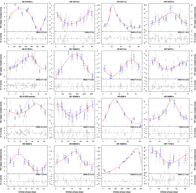
Figure 1. Phase curve and corresponding residuals for all planet candidates. The blue error bars show the error-weighted average RVs in 10 bins. The best orbital solution is determined by the MAP values of orbital parameters. The rms of the residual RVs is shown in each panel.
Download figure:
Standard image High-resolution imageTable 2. Parameters for Planet Candidates
| Planet | MpsinI (M⊕) | a (au) | P (days) | K (m s−1) | e | ω (deg) | M0 (deg) |
|---|---|---|---|---|---|---|---|
| HD 210193 b | 153.1 ± 23.3 | 1.487 ± 0.031 | 649.918 ± 8.599 | 11.40 ± 1.66 | 0.24 ± 0.09 | 168.84 ± 28.69 | 73.93 ± 32.63 |

|

|

|

|

|

|

|
|
| HD 211970 b | 13.0 ± 2.5 | 0.143 ± 0.003 | 25.201 ± 0.025 | 4.02 ± 0.74 | 0.15 ± 0.10 | 97.83 ± 51.73 | 84.80 ± 48.66 |

|

|

|

|

|

|

|
|
| HD 39855 b | 8.5 ± 1.5 | 0.041 ± 0.001 | 3.2498 ± 0.0004 | 4.08 ± 0.71 | 0.14 ± 0.11 | 102.97 ± 79.77 | 154.27 ± 77.93 |

|

|

|

|

|

|

|
|
| HIP 35173 b | 12.7 ± 2.7 | 0.217 ± 0.004 | 41.516 ± 0.077 | 2.80 ± 0.59 | 0.16 ± 0.11 | 10.73 ± 96.40 | -7.66 ± 91.92 |

|

|

|

|

|

|

|
|
| HD 102843 b | 113.9 ± 14.5 | 4.074 ± 0.270 | 3090.942 ± 295.049 | 5.24 ± 0.61 | 0.11 ± 0.07 | 108.69 ± 49.38 | 104.42 ± 54.78 |

|

|

|

|

|

|

|
|
| HD 103949 b | 11.2 ± 2.3 | 0.439 ± 0.009 | 120.878 ± 0.446 | 1.77 ± 0.35 | 0.19 ± 0.12 | 127.74 ± 68.28 | 234.49 ± 67.94 |

|

|

|

|

|

|

|
|
| HD 206255 b | 34.2 ± 7.1 | 0.461 ± 0.009 | 96.045 ± 0.317 | 3.92 ± 0.80 | 0.23 ± 0.11 | 86.92 ± 44.90 | 124.46 ± 46.09 |

|

|

|

|

|

|

|
|
| HD 21411 b | 65.9 ± 25.6 | 0.362 ± 0.007 | 84.288 ± 0.127 | 11.47 ± 4.33 | 0.40 ± 0.15 | 332.42 ± 17.74 | 285.65 ± 22.51 |

|

|

|

|

|

|

|
|
| HD 64114 b | 17.8 ± 3.5 | 0.246 ± 0.005 | 45.791 ± 0.070 | 3.33 ± 0.64 | 0.12 ± 0.08 | 215.30 ± 85.53 | 209.15 ± 85.31 |

|

|

|

|

|

|

|
|
| HD 8326 b | 66.6 ± 19.6 | 0.533 ± 0.011 | 158.991 ± 1.440 | 9.36 ± 2.72 | 0.20 ± 0.11 | -44.79 ± 36.46 | 272.91 ± 39.43 |

|

|

|

|

|

|

|
|
| HD 164604 b | 635.0 ± 82.3 | 1.331 ± 0.029 | 641.472 ± 10.129 | 60.66 ± 6.97 | 0.35 ± 0.10 | 65.40 ± 15.11 | 40.01 ± 25.82 |

|

|

|

|

|

|

|
|
| HIP 54373 b | 8.62 ± 1.84 | 0.063 ± 0.001 | 7.760 ± 0.003 | 4.19 ± 0.87 | 0.20 ± 0.11 | 72.34 ± 44.58 | 90.73 ± 43.89 |

|

|

|

|

|

|

|
|
| HIP 54373 c | 12.44 ± 2.11 | 0.099 ± 0.002 | 15.144 ± 0.008 | 4.84 ± 0.79 | 0.20 ± 0.12 | 122.37 ± 60.04 | 242.71 ± 57.33 |

|

|

|

|

|

|

|
|
| HD 24085 b | 11.8 ± 3.1 | 0.034 ± 0.001 | 2.0455 ± 0.0002 | 5.40 ± 1.37 | 0.22 ± 0.12 | 8.92 ± 54.83 | 156.74 ± 60.90 |

|

|

|

|

|

|

|
|
| HIP 71135 b | 18.8 ± 4.1 | 0.335 ± 0.007 | 87.190 ± 0.381 | 3.71 ± 0.79 | 0.21 ± 0.13 | 115.60 ± 71.72 | 223.03 ± 73.08 |

|

|

|

|

|

|

|
Note. The minimum mass, semimajor axis, period, RV semi-amplitude, eccentricity, and mean anomaly at the reference epoch are denoted by MpsinI, a, P, K, e, ω, and M0, respectively. The mean and standard deviation of each parameter are estimated from the posterior samples drawn by MCMC. For each parameter, the value at the MAP and the uncertainty interval defined by the 1% and 99% quantiles of the posterior distribution are shown below the values of the mean and standard deviation. The orbit of HD 164604 b is significantly eccentric because e = 0 is more than 3σ away from the mean. The orbital eccentricities for all other planet candidates are consistent with zero.
Download table as: ASCIITypeset image
The RV signal corresponding to a candidate is typically consistently found in different data chunks, as shown in the moving periodogram (e.g., see Figure 2 for HD 210193). As mentioned in Section 3, the moving periodogram may not be suitable for all signals, thus, we only show them for the RV signals that need further confirmation. We also calculate the BFPs for activity indices and do not find any overlap between activity signals and the Keplerian signals. We display these in a series of plots from Figure 3 onward where subplots P1 are for Hα etc. The 14 PFS data sets are shown in Table 3.
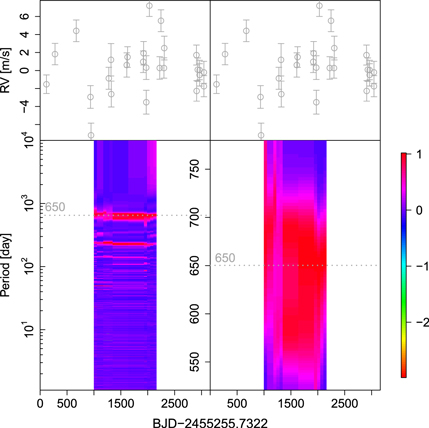
Figure 2. Moving periodogram for the PFS data for HD 210193. The top panels show RV data. The bottom right panel is a zoomed-in version of the bottom left panel, which shows the color-coded two-dimensional BFP. The x-axis is the BJD time relative to the first epoch. The periodogram power is normalized for each moving time window so that the BF does not depend on the number of RVs in each window. A global color coding is applied to these normalized BFs. The time span of each time window is 2036 days. The window move to cover the full data set within 20 steps. In the calculation of BFPs, we ignore the eccentricity of signals. This is not likely to change the time consistency of MCMC signals, although such assumption may alternate signal period and amplitude slightly.
Download figure:
Standard image High-resolution image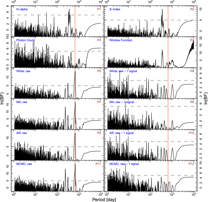
Figure 3. BFPs for HD 210193. The BFPs are calculated for the activity indices and for the white noise model, MA(1), and AR(1) for the raw RV data and RVs with sinusoidal signals subtracted. The BFPs for activity indices are calculated using the MA(1) model. The window function is calculated using the Lomb–Scargle periodogram (Lomb 1976; Scargle 1982). The activity indices, window function, noise models, and data sets are shown in the top left corners. Each panel is denoted by "Px" in the top right corner where "x" is a natural number. The RV signal at a period of 650 days is marked by the red vertical lines. The panels denoted by "MCMC" show the BFPs for the raw data subtracted by the best-fit Keplerian signals constrained by MCMC. The gray dashed line denotes the ln(BF) = 5 criterion in each BFP. The elements in this figure are also applicable for the subsequent figures. The signals in the residual BFPs are either noise-model dependent or not identified as significant signals through MCMC sampling.
Download figure:
Standard image High-resolution imageTable 3. PFS Data for the 14 Targets
| Star | BJD(TDB) | RV | RV Error | S-index | Hα | Photon Count |
|---|---|---|---|---|---|---|
| (days) | (m s−1) | (m s−1) | ||||
| HD 210193 | 2455255.7322 | −2.96 | 1.03 | 0.2681 | 0.03949 | 17240 |
| HD 210193 | 2455427.74325 | 10.5 | 1.19 | 0.1453 | 0.0298 | 20808 |
| HD 210193 | 2455853.59631 | −3.87 | 1.2 | 0.1457 | 0.03015 | 29319 |
| HD 210193 | 2456139.71964 | 6.04 | 1.26 | 0.1408 | 0.03059 | 34033 |
| HD 210193 | 2456150.73734 | 1.68 | 1.34 | 0.1459 | 0.03024 | 17527 |
| HD 210193 | 2456507.78955 | −8.57 | 1.22 | 0.1407 | 0.03049 | 33751 |
| HD 210193 | 2456551.68262 | −0.75 | 1.8 | 0.1522 | −1 | 23658 |
| HD 210193 | 2456556.69412 | −3.99 | 1.44 | 0.1589 | 0.031 | 16623 |
| HD 210193 | 2456867.80008 | 7.54 | 1.35 | 0.153 | 0.02991 | 29091 |
| HD 210193 | 2456883.72837 | 7.57 | 1.15 | 0.1475 | 0.03002 | 41296 |
| HD 210193 | 2457198.88933 | −1.32 | 1.2 | 0.1479 | 0.02977 | 33208 |
| HD 210193 | 2457205.83287 | 0.43 | 1.3 | 0.1532 | 0.02989 | 40291 |
| HD 210193 | 2457258.62318 | 3.76 | 1.32 | 0.1588 | 0.03054 | 27175 |
| HD 210193 | 2457259.74463 | 0 | 1.32 | 0.1558 | 0.03054 | 21843 |
| HD 210193 | 2457321.59187 | 14.24 | 1.2 | 0.1562 | 0.02954 | 24402 |
| HD 210193 | 2457529.88662 | 6.59 | 1.25 | 0.1457 | 0.0302 | 23762 |
| HD 210193 | 2457554.90868 | 10.2 | 1.21 | 0.1586 | 0.03064 | 21573 |
| HD 210193 | 2457614.76154 | −1.31 | 1.13 | 0.1468 | 0.03049 | 36335 |
| HD 210193 | 2457620.6494 | 0.09 | 1.32 | 0.1514 | −1 | 20191 |
| HD 210193 | 2458266.85745 | −0.13 | 1.11 | −1 | −1 | 16288 |
| HD 210193 | 2458270.89806 | −4.68 | 1.14 | −1 | −1 | 22104 |
| HD 210193 | 2458293.82287 | −5.82 | 1.3 | −1 | −1 | 18573 |
| HD 210193 | 2458329.77738 | −11.74 | 1.08 | −1 | −1 | 7636 |
| HD 210193 | 2458329.78116 | −12.28 | 1.24 | −1 | −1 | 7132 |
| HD 210193 | 2458416.55692 | −15.24 | 1.17 | −1 | −1 | 7138 |
| HD 210193 | 2458416.5608 | −13.7 | 1.22 | −1 | −1 | 7617 |
| HD 211970 | 2455255.7322 | −2.96 | 1.03 | 0.2681 | 0.03949 | 17240 |
| HD 211970 | 2455427.75376 | 4.39 | 1.01 | 1.0036 | 0.05437 | 24542 |
| HD 211970 | 2455439.7522 | 4.22 | 1.16 | 0.9017 | 0.05306 | 20281 |
| HD 211970 | 2455785.66778 | −6.38 | 1.17 | 0.6735 | 0.05198 | 22935 |
| HD 211970 | 2455787.78384 | −5.22 | 1.11 | 0.7317 | 0.05236 | 25121 |
| HD 211970 | 2455790.64196 | −0.3 | 1.15 | 0.7294 | 0.05265 | 20023 |
| HD 211970 | 2455793.66157 | −5.06 | 1.2 | 0.8489 | 0.05269 | 17699 |
| HD 211970 | 2455795.73434 | 2 | 1.11 | 0.724 | 0.05198 | 21689 |
| HD 211970 | 2455801.6949 | 2.91 | 1.24 | 0.8221 | 0.05361 | 12861 |
| HD 211970 | 2455802.66507 | 3.1 | 1.26 | 0.7252 | 0.05326 | 14089 |
| HD 211970 | 2455843.73573 | 0.23 | 1.26 | 0.4834 | 0.05189 | 15628 |
| HD 211970 | 2455844.62917 | −1.09 | 1.05 | 0.6433 | 0.05282 | 17331 |
| HD 211970 | 2455845.65818 | −3.1 | 1.07 | 0.6588 | 0.05241 | 16444 |
| HD 211970 | 2455846.6955 | −1.07 | 1.1 | 0.6576 | 0.05249 | 21090 |
| HD 211970 | 2455850.66816 | 3.63 | 1.2 | 0.6687 | 0.0551 | 13526 |
| HD 211970 | 2455851.6625 | 1.67 | 1.27 | 0.5961 | 0.05486 | 14869 |
| HD 211970 | 2455852.63469 | −0.86 | 1.29 | 0.6993 | 0.05403 | 13643 |
| HD 211970 | 2455853.60615 | −1.63 | 1.43 | 0.5476 | 0.05468 | 10524 |
| HD 211970 | 2456085.91961 | −4.78 | 1.14 | 0.7777 | 0.05213 | 20813 |
| HD 211970 | 2456086.82561 | −3.88 | 1.02 | 0.8023 | 0.05236 | 25862 |
| HD 211970 | 2456087.91929 | −5.73 | 1.45 | 0.9308 | 0.05402 | 10622 |
| HD 211970 | 2456092.87766 | 0.67 | 1.07 | 0.874 | 0.0524 | 23615 |
| HD 211970 | 2456141.7073 | 0.99 | 1.12 | 0.8227 | 0.05365 | 23515 |
| HD 211970 | 2456147.73551 | 5.39 | 1.57 | 0.8008 | −1 | 9014 |
| HD 211970 | 2456501.7777 | 6.74 | 1.24 | 0.8439 | 0.05292 | 18659 |
| HD 211970 | 2456504.84093 | 1.5 | 1.86 | 0.9769 | 0.05405 | 6983 |
| HD 211970 | 2456504.84951 | 6 | 1.71 | 0.9942 | 0.05364 | 7662 |
| HD 211970 | 2456506.79608 | 0.47 | 1.86 | 0.9598 | 0.05385 | 6825 |
| HD 211970 | 2456506.80612 | 9.49 | 3.55 | 0.9492 | 0.05433 | 3374 |
| HD 211970 | 2456555.60902 | 3.43 | 1.15 | 0.729 | 0.05246 | 19106 |
| HD 211970 | 2456556.72102 | −2.35 | 1.17 | 0.8122 | 0.05351 | 15289 |
| HD 211970 | 2456603.58858 | 6.93 | 1.03 | 0.576 | 0.05298 | 24254 |
| HD 211970 | 2456610.55366 | −13.6 | 1.03 | 0.5361 | 0.05267 | 22999 |
| HD 211970 | 2456816.93005 | −10.69 | 1.79 | 0.881 | 0.0543 | 7642 |
| HD 211970 | 2456818.87738 | −4.42 | 1.08 | 0.7789 | 0.05211 | 25940 |
| HD 211970 | 2456866.72527 | −5.89 | 1.05 | 0.7527 | 0.05193 | 27615 |
| HD 211970 | 2456871.73924 | −2.41 | 1.13 | 0.7926 | 0.05235 | 16594 |
| HD 211970 | 2456876.83292 | 2.96 | 1.24 | 0.8458 | 0.05245 | 19119 |
| HD 211970 | 2456879.717 | 0.6 | 1.08 | 0.8207 | 0.05307 | 26605 |
| HD 211970 | 2457198.89566 | −1.7 | 1.08 | 0.8817 | 0.05225 | 20889 |
| HD 211970 | 2457203.81436 | 2.47 | 1.15 | 0.9188 | 0.0538 | 23365 |
| HD 211970 | 2457260.7319 | 0 | 1.18 | 0.7327 | 0.05214 | 17234 |
| HD 211970 | 2457321.5985 | −5.3 | 1.07 | 0.4997 | 0.05319 | 19970 |
| HD 211970 | 2457536.92111 | 8.42 | 1.24 | 0.9646 | 0.05503 | 15202 |
| HD 211970 | 2457555.8774 | −2.5 | 1.05 | 0.8753 | 0.05301 | 24541 |
| HD 211970 | 2457614.77018 | 4.04 | 1.14 | 0.9375 | 0.05419 | 26397 |
| HD 211970 | 2457621.70646 | −0.82 | 1.05 | 0.8482 | 0.05353 | 20522 |
| HD 211970 | 2458293.84928 | 4.73 | 1.07 | −1 | −1 | 8166 |
| HD 211970 | 2458329.78811 | −3.74 | 0.96 | −1 | −1 | 7189 |
| HD 211970 | 2458355.67643 | −5.71 | 0.87 | −1 | −1 | 6828 |
| HD 211970 | 2458357.60275 | −5.85 | 1.04 | −1 | −1 | 4154 |
| HD 211970 | 2458357.60651 | −5.93 | 0.85 | −1 | −1 | 4515 |
| HD 39855 | 2455255.7322 | −2.96 | 1.03 | 0.2681 | 0.03949 | 17240 |
| HD 39855 | 2455200.69318 | 3.74 | 1.57 | 0.2162 | −1 | 17422 |
| HD 39855 | 2455255.58202 | −3.12 | 1.13 | 0.1975 | 0.03123 | 32336 |
| HD 39855 | 2455587.59977 | 1.07 | 1.26 | 0.1736 | 0.03222 | 20347 |
| HD 39855 | 2455587.60343 | 1.21 | 1.21 | 0.1694 | 0.033 | 20166 |
| HD 39855 | 2455669.49598 | 2.9 | 1.09 | 0.1835 | 0.03233 | 46028 |
| HD 39855 | 2455845.83806 | 0.78 | 1.31 | 0.1667 | 0.03186 | 21890 |
| HD 39855 | 2455852.86337 | 0 | 1.42 | 0.1635 | 0.03258 | 19112 |
| HD 39855 | 2455956.63819 | −1.3 | 1.31 | 0.159 | 0.03182 | 36101 |
| HD 39855 | 2456281.72155 | −2.11 | 1.37 | 0.1665 | −1 | 23915 |
| HD 39855 | 2456284.67998 | 0.75 | 1.19 | 0.1669 | 0.03205 | 49974 |
| HD 39855 | 2456345.5798 | 8.65 | 1.22 | 0.0324 | 0 | 24537 |
| HD 39855 | 2456356.60133 | −4.48 | 1.17 | 0.166 | 0.03208 | 31425 |
| HD 39855 | 2456358.57618 | 7.48 | 1.65 | 0.2344 | 0.03372 | 9358 |
| HD 39855 | 2456695.62685 | −0.22 | 1.28 | 0.1807 | 0.03197 | 36301 |
| HD 39855 | 2456703.59108 | 1.3 | 1.13 | 0.1992 | 0.03261 | 31290 |
| HD 39855 | 2457029.69333 | −3.62 | 1.25 | 0.1645 | 0.03183 | 53474 |
| HD 39855 | 2457053.61031 | −0.06 | 1.3 | 0.1691 | 0.0319 | 40647 |
| HD 39855 | 2457123.51006 | −1.78 | 1.1 | 0.1692 | 0.03184 | 33114 |
| HD 39855 | 2457267.88973 | 1.74 | 1.23 | 0.1609 | 0.03221 | 36153 |
| HD 39855 | 2457325.81241 | −3.09 | 1.27 | 0.1599 | 0.03185 | 43264 |
| HD 39855 | 2457389.6711 | −0.3 | 1.31 | 0.1606 | 0.03181 | 45327 |
| HD 39855 | 2457395.70227 | 0.32 | 1.5 | 0.1663 | 0.03228 | 17590 |
| HD 39855 | 2457448.5851 | −3.36 | 1.11 | 0.1677 | 0.03151 | 53217 |
| HD 39855 | 2457471.52459 | −2.9 | 1.31 | 0.1635 | 0.03179 | 30674 |
| HIP 35173 | 2455255.7322 | −2.96 | 1.03 | 0.2681 | 0.03949 | 17240 |
| HIP 35173 | 2455200.71753 | 6.59 | 1.68 | 0.3799 | −1 | 7620 |
| HIP 35173 | 2455252.62714 | −5.32 | 1.19 | 0.2378 | −1 | 18749 |
| HIP 35173 | 2455581.64495 | −3.75 | 1.05 | 0.2705 | 0.04027 | 23076 |
| HIP 35173 | 2455956.68819 | −3.17 | 1.02 | 0.2119 | 0.03946 | 24086 |
| HIP 35173 | 2455957.64998 | −0.34 | 1.69 | 0.3684 | 0.04145 | 5933 |
| HIP 35173 | 2456284.73876 | 2.24 | 0.99 | 0.2187 | 0.03928 | 25479 |
| HIP 35173 | 2456291.77672 | −4.32 | 0.91 | 0.2199 | 0.03931 | 21960 |
| HIP 35173 | 2456343.62157 | −2.2 | 0.99 | 0.2358 | 0.03954 | 21343 |
| HIP 35173 | 2456354.57027 | 0.3 | 0.99 | 0.2249 | 0.03952 | 18295 |
| HIP 35173 | 2456357.61684 | 4.18 | 0.94 | 0.2159 | 0.03952 | 19493 |
| HIP 35173 | 2456610.82296 | 1.19 | 1.01 | 0.2045 | 0.03912 | 21836 |
| HIP 35173 | 2456692.67294 | 1.23 | 1 | 0.2117 | 0.03897 | 25266 |
| HIP 35173 | 2456696.62238 | −0.12 | 1.06 | 0.2266 | 0.03968 | 19352 |
| HIP 35173 | 2456698.67353 | 1.45 | 0.85 | 0.2184 | 0.03961 | 22937 |
| HIP 35173 | 2456729.6363 | 3.45 | 0.96 | 0.1861 | 0.03963 | 25493 |
| HIP 35173 | 2456730.59016 | 3.84 | 1.04 | 0.2392 | 0.03957 | 19102 |
| HIP 35173 | 2456733.59673 | 3.92 | 0.93 | 0.2016 | 0.03951 | 23207 |
| HIP 35173 | 2457020.72449 | 5.8 | 0.93 | 0.2355 | 0.03905 | 25335 |
| HIP 35173 | 2457022.71547 | 5.23 | 0.88 | 0.2298 | 0.03988 | 26572 |
| HIP 35173 | 2457030.75951 | 0.67 | 0.99 | 0.2397 | 0.04002 | 23900 |
| HIP 35173 | 2457050.6369 | −0.88 | 0.93 | 0.2361 | 0.03982 | 25437 |
| HIP 35173 | 2457053.622 | −2.14 | 1.05 | 0.2335 | 0.04009 | 16408 |
| HIP 35173 | 2457060.6255 | 0.71 | 0.99 | 0.2171 | 0.03874 | 21750 |
| HIP 35173 | 2457069.61469 | 1.56 | 1.07 | 0.2294 | 0.03968 | 16376 |
| HIP 35173 | 2457118.54054 | −0.58 | 0.93 | 0.2351 | 0.03967 | 26280 |
| HIP 35173 | 2457122.53949 | −0.06 | 0.89 | 0.2355 | 0.03954 | 23231 |
| HIP 35173 | 2457324.87053 | −3.88 | 1.42 | 0.3246 | 0.04145 | 9338 |
| HIP 35173 | 2457327.85226 | 1.26 | 1.13 | 0.2742 | 0.04025 | 14149 |
| HIP 35173 | 2457387.66829 | −3.02 | 0.88 | 0.2645 | 0.04026 | 24824 |
| HIP 35173 | 2457396.65701 | −0.68 | 1.04 | 0.2645 | 0.03957 | 19286 |
| HIP 35173 | 2457448.62086 | −2.62 | 1.05 | 0.2613 | 0.04009 | 25338 |
| HIP 35173 | 2457471.54655 | 2.21 | 1.07 | 0.2645 | 0.04011 | 15211 |
| HIP 35173 | 2457499.53549 | −2.28 | 0.87 | 0.2483 | 0.03952 | 30511 |
| HIP 35173 | 2457737.74108 | −3.26 | 1.08 | 0.2444 | 0.039 | 26502 |
| HIP 35173 | 2457758.74084 | 1.8 | 0.9 | 0.2517 | 0.04008 | 22330 |
| HIP 35173 | 2457762.65955 | 0 | 1.07 | 0.2701 | 0.03987 | 23516 |
| HIP 35173 | 2457824.59241 | −0.76 | 0.99 | 0.2622 | 0.03915 | 18743 |
| HIP 35173 | 2458469.83192 | −0.13 | 1 | −1 | −1 | 4885 |
| HD 102843 | 2455255.7322 | −2.96 | 1.03 | 0.2681 | 0.03949 | 17240 |
| HD 102843 | 2455200.83576 | 0 | 2.43 | 0.2557 | −1 | 5708 |
| HD 102843 | 2455252.79165 | −1.84 | 1.26 | 0.1589 | −1 | 14798 |
| HD 102843 | 2455342.58244 | −0.1 | 1.26 | 0.1976 | 0.03497 | 14379 |
| HD 102843 | 2455585.824 | 2.86 | 1.31 | 0.1616 | 0.03431 | 15311 |
| HD 102843 | 2455664.67782 | −1.93 | 1.32 | 0.21 | 0.0337 | 15991 |
| HD 102843 | 2456093.53284 | 7.9 | 1.06 | 0.3384 | 0.03394 | 13810 |
| HD 102843 | 2456288.8541 | 4.36 | 1.15 | 0.1613 | 0.0343 | 19078 |
| HD 102843 | 2456345.79961 | 7.62 | 1.18 | 0.1877 | 0.03412 | 17302 |
| HD 102843 | 2456435.55492 | 4.65 | 1.22 | 0.1722 | 0.03345 | 19933 |
| HD 102843 | 2456694.81016 | 7.42 | 1.13 | 0.1816 | 0.03405 | 20088 |
| HD 102843 | 2456698.78069 | 5.44 | 1.17 | 0.1787 | 0.03419 | 18673 |
| HD 102843 | 2456701.73522 | 5.79 | 1.21 | 0.173 | 0.03419 | 17658 |
| HD 102843 | 2456730.72343 | 3.96 | 1.22 | 0.1926 | 0.03423 | 15830 |
| HD 102843 | 2456817.53906 | 6.99 | 1.37 | 0.2421 | 0.03412 | 14105 |
| HD 102843 | 2457023.84581 | 4.55 | 1.1 | 0.1748 | 0.03459 | 17749 |
| HD 102843 | 2457029.83073 | 3.92 | 1.08 | 0.1635 | 0.0334 | 20407 |
| HD 102843 | 2457065.81831 | 6.29 | 1.25 | 0.1613 | 0.03409 | 14638 |
| HD 102843 | 2457069.72688 | 4.24 | 1.22 | 0.1656 | 0.03448 | 14364 |
| HD 102843 | 2457119.70904 | 0.6 | 1.22 | 0.1677 | 0.03355 | 17706 |
| HD 102843 | 2457203.49054 | −0.26 | 1.17 | 0.158 | 0.03388 | 18199 |
| HD 102843 | 2457206.51837 | −0.76 | 1.1 | 0.1546 | 0.03372 | 20241 |
| HD 102843 | 2457390.84293 | 3.21 | 1.14 | 0.1521 | 0.03421 | 17726 |
| HD 102843 | 2457397.84159 | −1.19 | 1.22 | 0.1608 | 0.03427 | 12809 |
| HD 102843 | 2457448.79186 | −0.79 | 1.23 | 0.1565 | 0.03404 | 22385 |
| HD 102843 | 2457472.68105 | −4.12 | 1.3 | 0.1531 | 0.03406 | 19522 |
| HD 102843 | 2457505.60482 | −2.59 | 1.29 | 0.1656 | 0.03407 | 15096 |
| HD 102843 | 2457760.85002 | −5.58 | 1.14 | 0.1479 | 0.0342 | 21243 |
| HD 102843 | 2457829.80843 | −3.93 | 1.6 | 0.2068 | 0.0341 | 11045 |
| HD 102843 | 2458204.66791 | −3.35 | 0.93 | −1 | −1 | 14073 |
| HD 102843 | 2458204.71316 | −4.14 | 1 | −1 | −1 | 13154 |
| HD 102843 | 2458205.72943 | −3.62 | 1.03 | −1 | −1 | 13330 |
| HD 102843 | 2458206.68341 | −3.11 | 1.05 | −1 | −1 | 12668 |
| HD 102843 | 2458207.70655 | −2.38 | 0.98 | −1 | −1 | 14300 |
| HD 102843 | 2458208.63571 | −2.28 | 0.94 | −1 | −1 | 19760 |
| HD 102843 | 2458209.65381 | −3.39 | 0.93 | −1 | −1 | 20254 |
| HD 103949 | 2455255.7322 | −2.96 | 1.03 | 0.2681 | 0.03949 | 17240 |
| HD 103949 | 2455200.85365 | 1.87 | 1.57 | 0.2838 | −1 | 7861 |
| HD 103949 | 2455252.80669 | −4.49 | 1.19 | 0.2311 | −1 | 18529 |
| HD 103949 | 2455342.59972 | 1.02 | 1.05 | 0.1979 | 0.04018 | 29944 |
| HD 103949 | 2455584.81107 | 1.87 | 1.03 | 0.2294 | 0.04103 | 23085 |
| HD 103949 | 2455664.70212 | −1.29 | 1.1 | 0.2303 | 0.04016 | 24463 |
| HD 103949 | 2456093.54236 | −0.55 | 0.99 | 0.2439 | 0.04117 | 16120 |
| HD 103949 | 2456284.85339 | 3.57 | 1 | 0.2749 | 0.0407 | 24711 |
| HD 103949 | 2456345.81626 | −3.56 | 1.03 | 0.2768 | 0.0409 | 26003 |
| HD 103949 | 2456356.81978 | −2.33 | 1.12 | 0.2896 | 0.04172 | 20181 |
| HD 103949 | 2456431.59876 | −0.01 | 1.59 | 0.2572 | 0.04084 | 21637 |
| HD 103949 | 2456434.58574 | −1.51 | 1.05 | 0.2804 | 0.04086 | 21799 |
| HD 103949 | 2456438.57712 | 0.27 | 1.13 | 0.2702 | 0.04101 | 19845 |
| HD 103949 | 2456501.4829 | −2.1 | 1.24 | 0.2944 | 0.04111 | 14991 |
| HD 103949 | 2456693.77863 | −4.52 | 0.98 | 0.2627 | 0.04093 | 33792 |
| HD 103949 | 2456696.74631 | −2.93 | 1.04 | 0.2767 | 0.0402 | 22235 |
| HD 103949 | 2456700.78295 | 0.22 | 0.96 | 0.2344 | 0.04033 | 23764 |
| HD 103949 | 2456702.70173 | −0.47 | 1.05 | 0.2669 | 0.04105 | 22201 |
| HD 103949 | 2456729.7549 | −1.08 | 0.94 | 0.2666 | 0.03986 | 41798 |
| HD 103949 | 2456730.73207 | 0.41 | 1.02 | 0.2827 | 0.04008 | 24473 |
| HD 103949 | 2456816.56657 | −1.35 | 1.28 | 0.2531 | 0.04054 | 23830 |
| HD 103949 | 2457022.81444 | 2.14 | 0.9 | 0.2581 | 0.04022 | 25317 |
| HD 103949 | 2457026.8595 | −0.68 | 0.96 | 0.2575 | 0.04001 | 19568 |
| HD 103949 | 2457051.86844 | −1.99 | 1 | 0.2518 | 0.0401 | 24487 |
| HD 103949 | 2457064.70854 | −1.16 | 1.03 | 0.2449 | 0.04014 | 21884 |
| HD 103949 | 2457118.69169 | −2.56 | 1.05 | 0.2416 | 0.04088 | 26524 |
| HD 103949 | 2457123.69519 | 0.34 | 1.05 | 0.2494 | 0.0411 | 21538 |
| HD 103949 | 2457200.48178 | −1 | 1.09 | 0.2458 | 0.04072 | 23451 |
| HD 103949 | 2457389.80697 | 0.96 | 1.04 | 0.2319 | 0.04031 | 18497 |
| HD 103949 | 2457396.86666 | 2.12 | 0.97 | 0.2184 | 0.04079 | 21717 |
| HD 103949 | 2457450.78222 | −0.99 | 1.1 | 0.2338 | 0.03996 | 23609 |
| HD 103949 | 2457472.71043 | −1 | 1.04 | 0.2142 | 0.04002 | 23336 |
| HD 103949 | 2457478.70621 | −0.58 | 0.99 | 0.2063 | 0.03953 | 37022 |
| HD 103949 | 2457505.62043 | 2.32 | 1.06 | 0.2133 | 0.03972 | 23868 |
| HD 103949 | 2457555.52785 | −0.85 | 1.13 | 0.2765 | 0.04002 | 22711 |
| HD 103949 | 2457760.859 | 1.99 | 0.92 | 0.2064 | 0.04058 | 36733 |
| HD 103949 | 2457761.81112 | 3.34 | 0.91 | 0.2053 | −1 | 36580 |
| HD 103949 | 2457765.79163 | 0 | 1.08 | 0.2084 | 0.04087 | 21426 |
| HD 103949 | 2457825.75799 | 1.52 | 0.95 | 0.2212 | 0.04043 | 26191 |
| HD 103949 | 2457862.66605 | 0.07 | 1.11 | 0.2366 | 0.03969 | 16008 |
| HD 103949 | 2458203.69321 | 1.08 | 0.87 | −1 | −1 | 21612 |
| HD 103949 | 2458204.75568 | 2.05 | 0.88 | −1 | −1 | 15853 |
| HD 103949 | 2458205.74082 | 2.23 | 0.88 | −1 | −1 | 22214 |
| HD 103949 | 2458206.67226 | 1.42 | 0.83 | −1 | −1 | 19816 |
| HD 103949 | 2458207.71827 | 1.48 | 0.81 | −1 | −1 | 21013 |
| HD 103949 | 2458208.62537 | 0.8 | 0.83 | −1 | −1 | 22948 |
| HD 103949 | 2458209.64388 | 0.82 | 0.79 | −1 | −1 | 20962 |
| HD 103949 | 2458264.57394 | −0.63 | 0.91 | −1 | −1 | 19389 |
| HD 206255 | 2455255.7322 | −2.96 | 1.03 | 0.2681 | 0.03949 | 17240 |
| HD 206255 | 2455427.71742 | −2.66 | 1.3 | 0.1349 | 0.02973 | 21832 |
| HD 206255 | 2455439.73885 | −4.03 | 1.32 | 0.1355 | 0.03028 | 18934 |
| HD 206255 | 2455796.7401 | 2.49 | 1.4 | 0.1427 | 0.03018 | 19100 |
| HD 206255 | 2455850.65044 | 2.32 | 1.26 | 0.1429 | 0.02996 | 19692 |
| HD 206255 | 2455850.65416 | 2.34 | 1.4 | 0.1444 | 0.02997 | 19669 |
| HD 206255 | 2456086.81919 | −1.77 | 1.18 | 0.1315 | 0.02905 | 39826 |
| HD 206255 | 2456092.85872 | −1.16 | 1.23 | 0.1297 | 0.03006 | 25348 |
| HD 206255 | 2456139.70543 | 1.73 | 1.27 | 0.1338 | 0.02995 | 23160 |
| HD 206255 | 2456144.7747 | 2.14 | 1.65 | 0.1404 | 0.03056 | 13672 |
| HD 206255 | 2456150.7277 | −0.11 | 1.44 | 0.131 | 0.02972 | 18626 |
| HD 206255 | 2456504.83089 | −3.38 | 1.32 | 0.1362 | 0.03007 | 20147 |
| HD 206255 | 2456506.78512 | 1.91 | 1.32 | 0.142 | 0.02958 | 20609 |
| HD 206255 | 2456550.62471 | 7.66 | 1.43 | 0.3088 | 0.02968 | 32231 |
| HD 206255 | 2456553.6186 | 4.55 | 1.47 | 0.1388 | 0.02961 | 21158 |
| HD 206255 | 2456604.54902 | −4.1 | 1.23 | 0.1347 | 0.02951 | 26861 |
| HD 206255 | 2456817.86837 | 0.09 | 1.23 | 0.1319 | 0.02993 | 31069 |
| HD 206255 | 2456866.69534 | −3.18 | 1.31 | 0.1284 | 0.02972 | 39119 |
| HD 206255 | 2456876.68366 | −9.05 | 1.29 | 0.1275 | 0.02919 | 39943 |
| HD 206255 | 2457198.86731 | −1.8 | 1.34 | 0.1267 | 0.02996 | 27749 |
| HD 206255 | 2457206.83583 | −2.37 | 1.43 | 0.1242 | 0.02971 | 38134 |
| HD 206255 | 2457258.61859 | −2.48 | 1.31 | 0.1298 | 0.02977 | 30047 |
| HD 206255 | 2457321.57596 | 5.79 | 1.37 | 0.1304 | 0.0296 | 26552 |
| HD 206255 | 2457327.61917 | 3.74 | 1.3 | 0.129 | 0.02982 | 24059 |
| HD 206255 | 2457536.90929 | −5.04 | 1.31 | 0.1341 | 0.0296 | 23177 |
| HD 206255 | 2457555.86064 | −5.31 | 1.21 | 0.1229 | 0.02888 | 43387 |
| HD 206255 | 2457614.71064 | 0 | 1.2 | 0.1293 | 0.02955 | 38830 |
| HD 206255 | 2457620.63101 | −4.69 | 1.37 | 0.1404 | −1 | 20427 |
| HD 206255 | 2458271.77631 | 2.13 | 1.19 | −1 | −1 | 17530 |
| HD 206255 | 2458293.81535 | 1.92 | 1.21 | −1 | −1 | 20410 |
| HD 206255 | 2458334.76763 | −1.66 | 1.18 | −1 | −1 | 6918 |
| HD 206255 | 2458334.77142 | 0.67 | 1.21 | −1 | −1 | 7649 |
| HD 206255 | 2458354.67918 | −2.19 | 1.44 | −1 | −1 | 4487 |
| HD 206255 | 2458354.68676 | 0 | 1.41 | −1 | −1 | 4517 |
| HD 21411 | 2455255.7322 | −2.96 | 1.03 | 0.2681 | 0.03949 | 17240 |
| HD 21411 | 2455200.62078 | 5.04 | 1.34 | 0.2286 | −1 | 13359 |
| HD 21411 | 2455430.89198 | −0.25 | 1.36 | 0.2078 | 0.03409 | 20044 |
| HD 21411 | 2455584.57744 | 2.11 | 1.18 | 0.2027 | 0.03301 | 21664 |
| HD 21411 | 2455852.79817 | −6.04 | 1.46 | 0.1842 | 0.03321 | 19016 |
| HD 21411 | 2456143.9235 | 19.35 | 1.93 | 0.1895 | −1 | 12955 |
| HD 21411 | 2456281.63855 | −2.43 | 1.33 | 0.2106 | −1 | 25027 |
| HD 21411 | 2456290.59309 | −3.22 | 0.92 | 0.1861 | 0.03291 | 39304 |
| HD 21411 | 2456343.53765 | −1.08 | 1.04 | 0.1941 | 0.03295 | 24919 |
| HD 21411 | 2456358.52243 | 4.55 | 2.91 | 0.3238 | 0.03612 | 3820 |
| HD 21411 | 2456551.8202 | −0.56 | 1.97 | 0.2034 | −1 | 23523 |
| HD 21411 | 2456605.70767 | −6.31 | 1.41 | 0.2024 | 0.03334 | 22103 |
| HD 21411 | 2456612.67223 | 3.34 | 1.25 | 0.1946 | 0.03323 | 30911 |
| HD 21411 | 2456697.5676 | −4.21 | 1.04 | 0.1869 | 0.03265 | 32159 |
| HD 21411 | 2456866.90825 | −2.66 | 1.32 | 0.1951 | 0.03274 | 26895 |
| HD 21411 | 2456882.92219 | −1.71 | 1.34 | 0.1947 | 0.03284 | 36006 |
| HD 21411 | 2457022.63789 | −3.14 | 1.01 | 0.196 | 0.03318 | 36914 |
| HD 21411 | 2457029.63113 | 3 | 0.96 | 0.1996 | 0.0331 | 30569 |
| HD 21411 | 2457053.52375 | −1.31 | 1.2 | 0.1995 | 0.03282 | 21376 |
| HD 21411 | 2457061.56943 | −1.68 | 1.05 | 0.1944 | 0.03258 | 23471 |
| HD 21411 | 2457260.8869 | 1.71 | 1.46 | 0.1854 | 0.03264 | 21551 |
| HD 21411 | 2457320.75509 | −0.14 | 1.28 | 0.1889 | 0.0329 | 22339 |
| HD 21411 | 2457389.61809 | 0 | 0.98 | 0.1808 | 0.03256 | 35380 |
| HD 21411 | 2457622.92626 | −0.93 | 1.29 | 0.1882 | 0.03299 | 25644 |
| HD 21411 | 2457741.62792 | 11.4 | 1.28 | 0.2188 | 0.03356 | 37117 |
| HD 21411 | 2457759.59214 | 12.12 | 0.98 | 0.4113 | 0.03345 | 26847 |
| HD 21411 | 2457765.62903 | 8.83 | 1.27 | 0.2267 | 0.03378 | 18377 |
| HD 21411 | 2458410.70071 | 0.12 | 1.15 | −1 | −1 | 6032 |
| HD 21411 | 2458410.70461 | 2.18 | 1.15 | −1 | −1 | 5966 |
| HD 21411 | 2458417.74652 | 17.64 | 1.39 | −1 | −1 | 3519 |
| HD 21411 | 2458417.75021 | 17.21 | 1.36 | −1 | −1 | 4550 |
| HD 64114 | 2455255.7322 | −2.96 | 1.03 | 0.2681 | 0.03949 | 17240 |
| HD 64114 | 2455200.75154 | −0.15 | 1.31 | 0.2264 | −1 | 13346 |
| HD 64114 | 2455255.63455 | −1.84 | 1.31 | 0.2038 | 0.03093 | 39062 |
| HD 64114 | 2455586.77045 | −2.2 | 1.24 | 0.1658 | 0.03165 | 20608 |
| HD 64114 | 2455588.6773 | −0.93 | 1.05 | 0.1662 | 0.03134 | 32884 |
| HD 64114 | 2455671.55327 | −3.56 | 1.12 | 0.2606 | 0.03134 | 45495 |
| HD 64114 | 2456288.7264 | 6.35 | 1.06 | 0.1931 | 0.03201 | 41494 |
| HD 64114 | 2456290.78816 | 6.76 | 1.02 | 0.1901 | 0.03203 | 46531 |
| HD 64114 | 2456345.63885 | −1.92 | 1.34 | 0.0318 | 0 | 27065 |
| HD 64114 | 2456695.68081 | 2.47 | 1.22 | 0.1977 | 0.03172 | 24676 |
| HD 64114 | 2456702.66536 | −0.27 | 1.03 | 0.174 | 0.03123 | 42052 |
| HD 64114 | 2456733.60378 | 0.43 | 1.09 | 0.1725 | 0.0309 | 37678 |
| HD 64114 | 2456734.61888 | 0.66 | 1.03 | 0.1925 | 0.03118 | 41885 |
| HD 64114 | 2457021.71572 | 4.38 | 1 | 0.1766 | 0.03171 | 37198 |
| HD 64114 | 2457024.75524 | 4.53 | 1.05 | 0.1732 | 0.03228 | 42179 |
| HD 64114 | 2457053.66366 | −1.5 | 1.38 | 0.179 | 0.03179 | 23599 |
| HD 64114 | 2457061.63104 | 0.62 | 1.12 | 0.1723 | 0.03153 | 23509 |
| HD 64114 | 2457066.61776 | 3.57 | 1.29 | 0.1754 | 0.03175 | 19556 |
| HD 64114 | 2457117.56268 | 1.4 | 1.12 | 0.257 | 0.03123 | 43344 |
| HD 64114 | 2457122.55954 | 1.09 | 1.14 | 0.1829 | 0.0312 | 43004 |
| HD 64114 | 2457387.7083 | 0.06 | 0.89 | 0.1676 | −1 | 44362 |
| HD 64114 | 2457395.66312 | −1.26 | 1.32 | 0.1695 | 0.03179 | 20384 |
| HD 64114 | 2457468.59249 | −1.25 | 1.09 | 0.1994 | 0.03131 | 44770 |
| HD 64114 | 2457499.55607 | −4.62 | 1.13 | 0.1788 | 0.03112 | 45070 |
| HD 64114 | 2457740.73137 | 0 | 1.2 | 0.1793 | 0.0316 | 34668 |
| HD 64114 | 2457761.70022 | 1.89 | 1.18 | 0.1765 | −1 | 36217 |
| HD 64114 | 2457769.75899 | −0.32 | 1.26 | 0.1745 | 0.03163 | 25866 |
| HD 64114 | 2457833.59771 | −0.31 | 1.02 | 0.2028 | 0.03161 | 25333 |
| HD 8326 | 2455255.7322 | −2.96 | 1.03 | 0.2681 | 0.03949 | 17240 |
| HD 8326 | 2455585.54494 | 1.02 | 0.93 | 0.2795 | 0.03895 | 23077 |
| HD 8326 | 2456141.9085 | 1.63 | 0.93 | 0.2996 | 0.03954 | 21201 |
| HD 8326 | 2456173.80187 | −2.34 | 1.18 | 0.3144 | 0.03946 | 19470 |
| HD 8326 | 2456612.6198 | 7.2 | 1.15 | 0.2793 | 0.03956 | 20615 |
| HD 8326 | 2456866.87142 | −3.69 | 0.97 | 0.3533 | 0.03979 | 24202 |
| HD 8326 | 2456877.86915 | 8.75 | 1.19 | 0.3872 | 0.03964 | 21502 |
| HD 8326 | 2457022.60447 | 2.08 | 0.78 | 0.3289 | 0.03911 | 24195 |
| HD 8326 | 2457261.87244 | 0 | 1.14 | 0.3374 | 0.04018 | 18113 |
| HD 8326 | 2457324.71174 | −7.66 | 1.05 | 0.2769 | 0.03915 | 21787 |
| HD 8326 | 2457389.55141 | 12.24 | 0.85 | 0.3446 | 0.03958 | 22770 |
| HD 8326 | 2457617.86045 | −2.06 | 0.95 | 0.2911 | 0.03929 | 22645 |
| HD 8326 | 2457739.57509 | 1.28 | 0.91 | 0.2429 | 0.03867 | 24241 |
| HD 8326 | 2457762.5492 | −7.57 | 1.01 | 0.2622 | 0.0384 | 18459 |
| HD 8326 | 2457767.5642 | −6.47 | 0.94 | 0.2491 | 0.03803 | 23125 |
| HD 8326 | 2458407.70844 | −2.62 | 0.97 | −1 | −1 | 7325 |
| HIP 31609 | 2455255.7322 | −2.96 | 1.03 | 0.2681 | 0.03949 | 17240 |
| HIP 31609 | 2458407.8526 | −10.6 | 1.38 | −1 | −1 | 1890 |
| HIP 31609 | 2458408.85256 | 0.43 | 1.44 | −1 | −1 | 2290 |
| HIP 31609 | 2458409.84653 | −0.03 | 1.61 | −1 | −1 | 1786 |
| HIP 31609 | 2458410.84883 | 5.98 | 1.39 | −1 | −1 | 1854 |
| HIP 31609 | 2458411.85426 | 6.32 | 1.21 | −1 | −1 | 2563 |
| HIP 31609 | 2458412.85539 | 7.35 | 1.37 | −1 | −1 | 2603 |
| HIP 31609 | 2458414.85554 | 6.52 | 1.68 | −1 | −1 | 1516 |
| HIP 31609 | 2458415.80466 | 0.65 | 1.52 | −1 | −1 | 2027 |
| HIP 31609 | 2458416.84913 | −5.34 | 1.36 | −1 | −1 | 2229 |
| HIP 31609 | 2458417.78781 | −4.53 | 1.8 | −1 | −1 | 1330 |
| HIP 31609 | 2458418.84782 | 3.99 | 1.37 | −1 | −1 | 2197 |
| HIP 31609 | 2458467.77358 | −6.71 | 1.19 | −1 | −1 | 2795 |
| HIP 31609 | 2458467.8106 | −4.61 | 1.51 | −1 | −1 | 2272 |
| HIP 31609 | 2458468.75877 | −9.98 | 1.27 | −1 | −1 | 2637 |
| HIP 31609 | 2458468.81937 | −12.14 | 1.21 | −1 | −1 | 2516 |
| HIP 31609 | 2458469.76285 | −7.79 | 1.35 | −1 | −1 | 1833 |
| HIP 31609 | 2458469.82074 | −10.52 | 1.54 | −1 | −1 | 1670 |
| HIP 31609 | 2458471.76184 | −7.42 | 1.41 | −1 | −1 | 2250 |
| HIP 31609 | 2458471.83237 | −12.98 | 1.43 | −1 | −1 | 1684 |
| HIP 31609 | 2458473.76748 | −5.48 | 1.13 | −1 | −1 | 2773 |
| HIP 31609 | 2458473.83554 | 0 | 1.34 | −1 | −1 | 1845 |
| HIP 31609 | 2458474.71356 | 0.35 | 1.26 | −1 | −1 | 2174 |
| HIP 31609 | 2458474.82237 | 0.53 | 1.57 | −1 | −1 | 1908 |
| HIP 31609 | 2458475.73745 | 6.98 | 1.38 | −1 | −1 | 2239 |
| HIP 31609 | 2458475.83545 | 10.06 | 1.28 | −1 | −1 | 2198 |
| HIP 31609 | 2458476.76185 | 11.97 | 1.45 | −1 | −1 | 2264 |
| HIP 31609 | 2458476.84509 | 9.29 | 1.28 | −1 | −1 | 2364 |
| HIP 54373 | 2455255.7322 | −2.96 | 1.03 | 0.2681 | 0.03949 | 17240 |
| HIP 54373 | 2455200.81388 | −0.01 | 3.3 | 1.1365 | −1 | 3251 |
| HIP 54373 | 2455254.65524 | −5.75 | 1.38 | 1.2993 | −1 | 9665 |
| HIP 54373 | 2455341.55657 | −1 | 1.44 | 1.0644 | 0.06204 | 8371 |
| HIP 54373 | 2455582.82444 | −1.95 | 1.35 | 1.4122 | 0.0628 | 8352 |
| HIP 54373 | 2455668.64626 | 3.41 | 1.53 | 1.1943 | 0.06075 | 6572 |
| HIP 54373 | 2455672.54785 | 11.35 | 1.81 | 1.1771 | 0.0637 | 5709 |
| HIP 54373 | 2455954.79749 | 3.3 | 1.45 | 1.5138 | 0.06136 | 7566 |
| HIP 54373 | 2455955.79678 | 4.54 | 1.53 | 1.4293 | 0.06109 | 6743 |
| HIP 54373 | 2455957.82077 | 9.43 | 3.81 | 1.3056 | 0.06466 | 2210 |
| HIP 54373 | 2455958.80249 | 4.63 | 1.7 | 1.4975 | 0.06263 | 5216 |
| HIP 54373 | 2455959.80289 | 3.33 | 1.51 | 1.5661 | 0.06282 | 6459 |
| HIP 54373 | 2455960.80708 | −0.08 | 1.57 | 1.4675 | 0.06325 | 5887 |
| HIP 54373 | 2456086.51118 | −0.64 | 1.48 | 0.9156 | 0.05982 | 8747 |
| HIP 54373 | 2456088.528 | 3.92 | 1.79 | 0.876 | 0.06047 | 5976 |
| HIP 54373 | 2456092.50926 | 2.43 | 2.68 | 1.0897 | 0.06162 | 3342 |
| HIP 54373 | 2456093.49839 | 0.85 | 1.5 | 0.8899 | 0.06177 | 4120 |
| HIP 54373 | 2456282.84604 | −5.35 | 1.51 | 1.4307 | 0.06256 | 7443 |
| HIP 54373 | 2456288.83793 | −1.11 | 1.3 | 1.5356 | 0.06108 | 7256 |
| HIP 54373 | 2456292.84185 | 7.97 | 1.32 | 1.4246 | 0.06095 | 7182 |
| HIP 54373 | 2456344.72208 | −3.99 | 1.68 | 1.4487 | 0.06154 | 6179 |
| HIP 54373 | 2456353.74857 | 14.91 | 1.58 | 1.0695 | 0.06313 | 6197 |
| HIP 54373 | 2456356.78344 | −11.1 | 1.66 | 1.4895 | 0.06219 | 5956 |
| HIP 54373 | 2456428.55774 | 8.18 | 1.86 | 1.0544 | 0.06211 | 5817 |
| HIP 54373 | 2456433.55267 | −13.61 | 1.77 | 1.0966 | 0.0624 | 6182 |
| HIP 54373 | 2456434.5606 | −12.48 | 3.04 | 1.1327 | 0.06307 | 2929 |
| HIP 54373 | 2456438.56787 | 7.56 | 2.2 | 1.0119 | 0.06025 | 4376 |
| HIP 54373 | 2456693.75493 | −4.85 | 1.33 | 1.4456 | 0.06084 | 8806 |
| HIP 54373 | 2456696.73138 | 3.04 | 1.41 | 1.5517 | 0.06225 | 7912 |
| HIP 54373 | 2456698.75589 | −2.94 | 1.43 | 1.4152 | 0.06235 | 7353 |
| HIP 54373 | 2456701.71882 | 4.8 | 1.51 | 1.4904 | 0.06203 | 6851 |
| HIP 54373 | 2456734.73037 | −0.39 | 1.36 | 1.3109 | 0.06347 | 8708 |
| HIP 54373 | 2456735.71095 | −1.82 | 1.42 | 1.421 | 0.06248 | 6898 |
| HIP 54373 | 2456818.49057 | 4.89 | 1.67 | 0.8612 | 0.0608 | 5877 |
| HIP 54373 | 2457021.84001 | 1.8 | 1.15 | 1.6562 | 0.06457 | 10807 |
| HIP 54373 | 2457026.82576 | −0.99 | 1.28 | 1.6873 | 0.06407 | 11485 |
| HIP 54373 | 2457051.75433 | 6.1 | 1.32 | 1.6401 | 0.06481 | 8960 |
| HIP 54373 | 2457062.72414 | 0 | 1.48 | 1.4429 | 0.0605 | 7730 |
| HIP 54373 | 2457120.68354 | 0 | 1.43 | 1.2376 | 0.06137 | 9716 |
| HIP 54373 | 2457203.47387 | −1.62 | 1.5 | 1.1355 | 0.06207 | 6658 |
| HIP 54373 | 2457387.8144 | −4.92 | 1.26 | 1.7353 | 0.06515 | 8091 |
| HIP 54373 | 2457397.80848 | 0.66 | 1.5 | 1.7506 | 0.06575 | 6829 |
| HIP 54373 | 2457448.74521 | −1.84 | 1.5 | 1.5171 | 0.06162 | 8295 |
| HIP 54373 | 2457473.66083 | 1.81 | 1.52 | 1.4173 | 0.06234 | 8871 |
| HIP 54373 | 2457478.66936 | 5.97 | 1.3 | 1.2089 | 0.06035 | 9693 |
| HIP 54373 | 2457499.6386 | −3.47 | 1.49 | 1.0454 | 0.06117 | 9651 |
| HIP 54373 | 2457559.48686 | −0.38 | 1.26 | 1.0418 | 0.06163 | 11132 |
| HIP 54373 | 2457759.83236 | 4.75 | 1.32 | 1.4273 | 0.06249 | 10217 |
| HIP 54373 | 2457824.71916 | −2.79 | 1.74 | 1.4785 | 0.06239 | 7142 |
| HIP 54373 | 2457848.57423 | 2.37 | 1.43 | 1.4862 | 0.0641 | 9027 |
| HIP 54373 | 2458264.55224 | −5 | 1.08 | −1 | −1 | 6014 |
| HD 24085 | 2455255.7322 | −2.96 | 1.03 | 0.2681 | 0.03949 | 17240 |
| HD 24085 | 2455582.60234 | −1.46 | 1.08 | 0.1352 | 0.02901 | 23031 |
| HD 24085 | 2455582.60495 | 5.07 | 1.2 | 0.1546 | 0.02952 | 15946 |
| HD 24085 | 2456145.91788 | 0.84 | 1.9 | 0.1528 | 0.0293 | 16842 |
| HD 24085 | 2456290.6024 | 0 | 1.09 | 0.1333 | 0.02865 | 44667 |
| HD 24085 | 2456551.82884 | 8.13 | 2.39 | 0.1996 | −1 | 23351 |
| HD 24085 | 2456606.70671 | 6.58 | 1.52 | 0.1481 | −1 | 18894 |
| HD 24085 | 2456698.55207 | 3.42 | 1.24 | 0.1376 | 0.02833 | 31582 |
| HD 24085 | 2456871.92807 | −0.14 | 1.72 | 0.1322 | 0.0281 | 34132 |
| HD 24085 | 2457022.6474 | −0.19 | 1.11 | 0.1333 | 0.02843 | 46090 |
| HD 24085 | 2457029.63619 | −1.5 | 1.01 | 0.4486 | 0.02856 | 34399 |
| HD 24085 | 2457053.53884 | −1.5 | 1.2 | 0.1425 | 0.02804 | 21504 |
| HD 24085 | 2457066.53534 | −1.9 | 1.32 | 0.1423 | 0.02915 | 18847 |
| HD 24085 | 2457262.87843 | −0.19 | 1.31 | 0.1383 | 0.02889 | 25690 |
| HD 24085 | 2457319.79348 | −6.56 | 1.31 | 0.1408 | 0.02874 | 23074 |
| HD 24085 | 2457389.61345 | −2.7 | 1.07 | 0.1307 | 0.0284 | 40886 |
| HD 24085 | 2457450.51648 | −3.32 | 1.54 | 0.2745 | 0.02785 | 36913 |
| HD 24085 | 2457621.92363 | 1.77 | 1.46 | 0.1484 | 0.02901 | 19681 |
| HD 24085 | 2457741.63286 | 1.73 | 1.24 | 0.1384 | 0.02812 | 39691 |
| HD 24085 | 2457761.60444 | 0.11 | 0.99 | 0.1469 | −1 | 36598 |
| HD 24085 | 2457766.5965 | 10.82 | 1.15 | 0.1383 | 0.02767 | 31505 |
| HD 24085 | 2458354.90321 | 0.8 | 1.44 | −1 | −1 | 5261 |
| HD 24085 | 2458410.70939 | 2.52 | 1.36 | −1 | −1 | 6274 |
| HD 24085 | 2458410.71321 | 0.55 | 1.36 | −1 | −1 | 5865 |
| HD 24085 | 2458417.75784 | −1.6 | 1.22 | −1 | −1 | 9685 |
| HIP 71135 | 2455255.7322 | −2.96 | 1.03 | 0.2681 | 0.03949 | 17240 |
| HIP 71135 | 2455342.66134 | −0.84 | 1.81 | 0.6097 | 0.05082 | 6564 |
| HIP 71135 | 2455423.50522 | 2.75 | 1.56 | 0.4679 | 0.05022 | 6871 |
| HIP 71135 | 2455437.47257 | 5.23 | 1.44 | 0.4713 | 0.04998 | 7527 |
| HIP 71135 | 2455785.52424 | 5.55 | 1.71 | 0.6408 | 0.05044 | 5343 |
| HIP 71135 | 2455787.50123 | 4.29 | 1.58 | 0.5024 | 0.05042 | 6782 |
| HIP 71135 | 2455793.49665 | 0 | 2.74 | 0.9498 | 0.05275 | 3198 |
| HIP 71135 | 2455796.52697 | 1.33 | 2.21 | 0.6912 | 0.05062 | 3804 |
| HIP 71135 | 2455801.50064 | −0.41 | 2.6 | 0.6665 | 0.05317 | 3256 |
| HIP 71135 | 2455802.48336 | −1.87 | 2.52 | 0.8015 | 0.05235 | 3236 |
| HIP 71135 | 2455802.49089 | 2.99 | 4.08 | 0.6045 | 0.05228 | 2347 |
| HIP 71135 | 2455803.49751 | 5.78 | 2.06 | 0.6305 | 0.05074 | 4124 |
| HIP 71135 | 2455804.51336 | 6.2 | 2.46 | 0.8024 | 0.05122 | 3173 |
| HIP 71135 | 2455958.86941 | 7.28 | 1.7 | 0.4351 | 0.04957 | 5545 |
| HIP 71135 | 2456085.68322 | 0.21 | 1.99 | 0.5965 | 0.05015 | 5509 |
| HIP 71135 | 2456094.5975 | 0.37 | 2.22 | 0.6373 | 0.05039 | 4013 |
| HIP 71135 | 2456344.81656 | −6.35 | 1.6 | 0.6323 | 0.04945 | 7260 |
| HIP 71135 | 2456347.86443 | −4.46 | 1.47 | 0.5509 | 0.04972 | 6454 |
| HIP 71135 | 2456352.84684 | −3.15 | 1.56 | 0.4161 | 0.04915 | 7537 |
| HIP 71135 | 2456355.82826 | −1.64 | 1.62 | 0.473 | 0.04994 | 5795 |
| HIP 71135 | 2456357.83352 | 0.88 | 2.26 | 0.7276 | 0.05083 | 3488 |
| HIP 71135 | 2456433.68066 | −9.55 | 1.96 | 0.5104 | 0.0495 | 5171 |
| HIP 71135 | 2456435.64872 | −3.37 | 1.79 | 0.502 | 0.04961 | 7090 |
| HIP 71135 | 2456505.53671 | −1.55 | 1.89 | 0.5166 | 0.05004 | 5215 |
| HIP 71135 | 2456505.54627 | −2.26 | 1.8 | 0.5029 | 0.05041 | 4960 |
| HIP 71135 | 2456693.83985 | −3.02 | 1.65 | 0.6546 | 0.04985 | 7995 |
| HIP 71135 | 2456696.85337 | −4.25 | 1.66 | 0.4446 | 0.04991 | 7582 |
| HIP 71135 | 2456698.88682 | 1.17 | 2.02 | 0.5201 | 0.05064 | 4152 |
| HIP 71135 | 2456729.81559 | −1.66 | 1.47 | 0.4786 | 0.04997 | 7362 |
| HIP 71135 | 2456733.82888 | 3.99 | 1.76 | 0.4666 | 0.04992 | 6573 |
| HIP 71135 | 2456734.82708 | −2.76 | 1.64 | 0.5633 | 0.05004 | 6805 |
| HIP 71135 | 2456817.66181 | −3.13 | 2.28 | 0.7852 | 0.05095 | 4477 |
| HIP 71135 | 2457067.85988 | 1.33 | 1.67 | 0.482 | 0.04926 | 6457 |
| HIP 71135 | 2457120.74646 | −3.59 | 1.71 | 0.5834 | 0.04968 | 8725 |
| HIP 71135 | 2457204.58631 | 2.37 | 1.65 | 0.4521 | 0.05029 | 7820 |
| HIP 71135 | 2457265.48913 | 1.58 | 1.5 | 0.5086 | 0.05034 | 7955 |
| HIP 71135 | 2457449.88976 | 1.41 | 1.51 | 0.4015 | 0.04978 | 11195 |
| HIP 71135 | 2457500.82204 | −6.79 | 1.69 | 0.5521 | 0.04979 | 8611 |
| HIP 71135 | 2457534.66035 | 4.6 | 1.92 | 0.7042 | 0.05033 | 5762 |
| HIP 71135 | 2457557.60976 | −9.73 | 1.77 | 0.452 | 0.04921 | 8042 |
| HIP 71135 | 2457626.49196 | 4 | 1.52 | 0.5047 | 0.04976 | 7897 |
| HIP 71135 | 2457825.8283 | −5.28 | 1.76 | 0.5633 | 0.04923 | 8850 |
| HIP 71135 | 2457850.80439 | −4.94 | 1.82 | 0.4754 | 0.05018 | 6916 |
| HIP 71135 | 2458264.68979 | −3.07 | 1.46 | −1 | −1 | 4145 |
Note. The nonvalid values in the tables are denoted by −1.
We discuss the results for individual cases as follows.
- 1.HD 210193 is a G star with a mass of 1.04 M⊙ and a distance of 42.25 pc. The planet candidate has a minimum mass of 153 M⊕ and an orbital period of about 650 days. It is a warm giant planet located in the temperate zone with the inner and outer boundaries corresponding to orbital periods of 256 and 926 days, respectively, according to Kopparapu et al. (2014).We also calculate the BFPs for activity indices and do not find any overlap between activity signals and the Keplerian signal, as shown in Figure 3. The phase curve in Figure 1 shows a good fit of the one-planet model to the RV data in terms of phase coverage and high statistical significance (i.e., ln(BF) = 10.9). The corresponding RV signal is consistently found in different data chunks, as shown in the moving periodogram (see Figure 2).There are also other short-period signals shown in the BFPs for residual RVs (P6, P8, P10, and P12 in Figure 3), but they are either not significant or depend on the choice of noise models.
- 2.HD 211970 (GJ 1267) is a K star with a mass of 0.61 M⊙. It is about 13 pc away from the Sun and is the nearest star in this reported sample. The planet candidate is consistent with a Neptune with a minimum mass of 13.92 M⊕ and an orbital period of 25.2 days.We also identify an activity signal at a period of 64.0 days. This activity signal shows strong power in the BFPs for RVs and the S-index (Figure 4). A Keplerian fit of the activity signal to the RV data shows nonzero eccentricity and large residuals with a rms of 4.2 m s−1 (see Figure 1), suggesting an origin caused by the quasi-periodic differential rotation of the star that cannot be properly modeled by deterministic periodic functions. Thus, the rotation period of this star is probably 64 days. Because the true model of activity signal is not known, we report the orbital parameters for the planet candidate based on the MCMC posterior sampling for a one-planet model.
- 3.HD 39855 is a G star with a mass of 0.87 M⊙ and a distance of 23.28 pc. The planet candidate is consistent with a hot super-Earth with a minimum mass of 8.5 M⊕ and an orbital period of 3.25 days. The corresponding RV signal is not evident in the BFPs for the S-index and Hα shown in Figure 5.
- 4.HIP 35173 is a K star with a mass of 0.79 M⊙ and a distance of 33.19 pc. The planet candidate is consistent with a Neptune with a minimum mass of 12.7 M⊕ and an orbital period of 41.5 days. The corresponding RV signal is not evident in the BFPs for the activity indices of the S-index and Hα shown in Figure 6. This signal is also consistently strong in various data chunks, as seen from the moving periodogram in Figure 7.
- 5.HD 102843 is a K star with a mass of 0.95 M⊙ and a distance of 62.87 pc. The planet candidate is consistent with a cool Saturn with a minimum mass of 114 M⊕ and an orbital period of 3090 days. Due to its long orbital period, the time span of the data is not long enough to cover multiple orbital periods and, thus, the moving periodogram is not appropriate for a test of time consistency. This signal is statistically significant (ln(BF) = 7.7; also see Figure 1) and is unique in the BFPs for various noise models (see Figure 8). On the other hand, the BFP for Hα shows a signal with a period much longer than the RV signal, probably arising from the magnetic cycle.
- 6.HD 103949 is a K star with a mass of 0.77 M⊙ and a distance of 26.52 pc. The planet candidate has a minimum mass of 11.2 M⊕ and an orbital period of 121 days. It is a warm Neptune located in the temperate zone. The corresponding RV signal is not evident in the BFPs for the activity indices of the S-index and Hα shown in Figure 9.
- 7.HD 206255 is a G star with a mass of 1.42 M⊙ and a distance of 75.40 pc. The planet candidate is consistent with a Neptune with a minimum mass of 34.2 M⊕ and an orbital period of 96.0 days.The corresponding RV signal is unique and has an eccentricity consistent with zero, as indicated by the posterior distribution. Thus, the extra number of free parameters of the one-planet model with respect to the zero-planet model is better when set to three instead of five in the calculation of BF. The former leads to ln(BF) = 8.1, while the latter to ln(BF) = 4.6. Although the latter does not pass the ln(BF) > 5 criterion, we count it as a valid planet candidate due to the above considerations in the calculation of ln(BF) and also because it satisfies all other criteria (see Figure 10).
- 8.HD 21411 is a G star with a mass of 0.89 M⊙ and a distance of 29.16 pc. The planet candidate is consistent with a Neptune with a minimum mass of 65.8 M⊕ and an orbital period of 84.3 days.However, the corresponding signal is not as strong as the 18.8 days signal in the BFP (see Figure 11), probably due to its high eccentricity (e = 0.4) and the assumption of circular orbit in the calculation of BFP. To confirm the signal, we launch multiple MCMC chains and find the same significant 18.8 days signal, leading to ln(BF) = 13.2. We also constrain the 84.3 and 18.8 days signals simultaneously and find that the two-planet model has a logarithmic BF of 2.8 with respect to the one-planet model. Thus, we conclude that the 84.3 days signal is significant, while the 18.8 days signal is not significant enough to report. The 18.8 days signal is not see in the BFPs for the S-index and Hα; further follow-up observations are needed to investigate the nature of this signal.
- 9.HD 64114 is a G star with a mass of 0.95 M⊙ and a distance of 31.55 pc. The planet candidate is consistent with a Neptune with a minimum mass of 17.8 M⊕ and an orbital period of 45.8 days. The corresponding RV signal is not evident in the BFPs for the activity indices of S-index and Hα shown in Figure 12.
- 10.HD 8326 is a K star with a mass of 0.8 M⊙ and a distance of 30.71 pc. The candidate is consistent with a planet with a minimum mass of 66.4 M⊕ and an orbital period of 159 days, which is consistent with the temperate zone around this star. The corresponding RV signal is not evident in the BFPs for the activity indices of the S-index and Hα shown in Figure 13.
- 11.HD 164604 is a K star with a mass of 0.77 M⊙ and a distance of 39.41 pc. The candidate is consistent with a Jupiter with a minimum mass of 635 M⊕ and an orbital period of 641 days. The corresponding RV signal is not evident in the BFPs for the activity indices of the S-index and Hα shown in Figure 14.
- 12.HIP 54373 is a K star with a mass of 0.57 M⊙ and a distance of 18.73 pc. There are two-planet candidates corresponding to (1) a hot super-Earth with a minimum mass of 8.6 M⊕ and an orbital period of 7.76 days and (2) a hot Neptune with a minimum mass of 12.4 M⊕ and an orbital period of 15.1 days. The orbits of these two planets form a 1:2 resonance. The eccentricities of these two candidate planets are consistent with zero since e = 0 is less than 2σ away from the means. The corresponding two RV signals are consistently identified in the BFPs for various noise models (see P5, P6, P8, P9, P11, and P12 in Figure 15) and do not show significant power excess in the BFPs for the S-index and Hα. They are also consistent in time, as seen from the moving periodograms shown in Figures 16 and 17. The two-planet solution is favored over the one-planet solution because ln(BF) = 5.2. The MAP value of the eccentricity for the 15.1 days signal decreases from 0.30 for the one-planet model to 0.24 for the two-planet model. Thus, the 7.76 days signal is favored by the data in terms of increasing the goodness of fit and reducing the eccentricity of the 15.1 days signal to a lower and, thus, more reasonable value (Kipping 2013). According to our analysis of the RV data, there are potentially additional signals, which warrants further observations and analyses.
- 13.HD 24085 is a G star with a mass of 1.22 M⊙ and a distance of 54.99 pc. The planet candidate is consistent with a hot Neptune with a minimum mass of 11.8 M⊕ and an orbital period of 2.04 days. The corresponding RV signal is not evident in the BFPs for the activity indices of the S-index and Hα shown in Figure 18.
- 14.HIP 71135 is an M star with a mass of 0.66 M⊙ and a distance of 32.36 pc. The planet candidate is consistent with a Neptune with a minimum mass of 18.8 M⊕ and an orbital period of 87.2 days, which is consistent with the temperate zone around this star. The corresponding RV signal is not evident in the BFPs for the activity indices of the S-index and Hα shown in Figure 19. The signal is consistent in time, as seen from the moving periodogram shown in Figure 20.

Figure 4. BFPs for HD 211970. The red line shows the Keplerian signal at a period of 25.2 days, while the green line shows the 64.0-day activity signal.
Download figure:
Standard image High-resolution image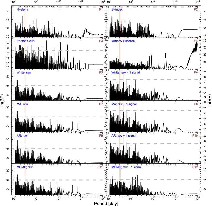
Figure 5. BFPs for HD 39855. The red line shows the signal at a period of 3.25 days.
Download figure:
Standard image High-resolution image
Figure 6. BFPs for HIP 35173. The red line shows the signal at a period of 41.5 days.
Download figure:
Standard image High-resolution image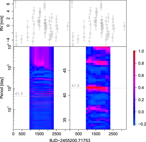
Figure 7. Moving periodogram for HIP 35173 b. The window size is 2000 days and the number of steps is 10. The other signals in the bottom right panel are the annual aliases of the 41.5-day signal.
Download figure:
Standard image High-resolution image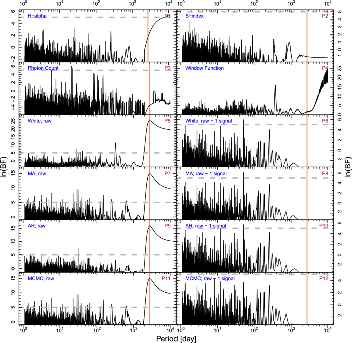
Figure 8. BFPs for HD 102843. The red line shows the signal at a period of about 3000 days.
Download figure:
Standard image High-resolution image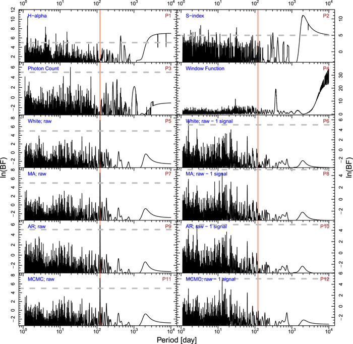
Figure 9. BFPs for HD 103949. The red line shows the signal at a period of 121 days.
Download figure:
Standard image High-resolution image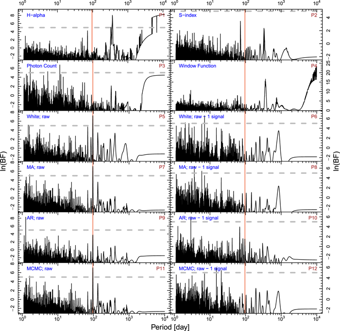
Figure 10. BFPs for HD 206255. The red line shows the signal at a period of 96.0 days.
Download figure:
Standard image High-resolution image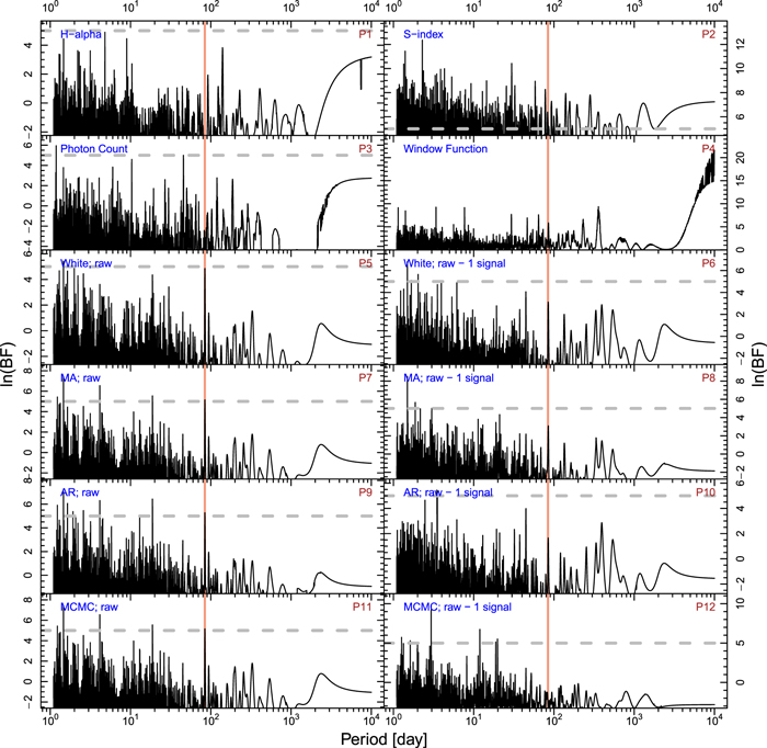
Figure 11. BFPs for HD 21411. The red line shows the signal at a period of 84.3 days.
Download figure:
Standard image High-resolution image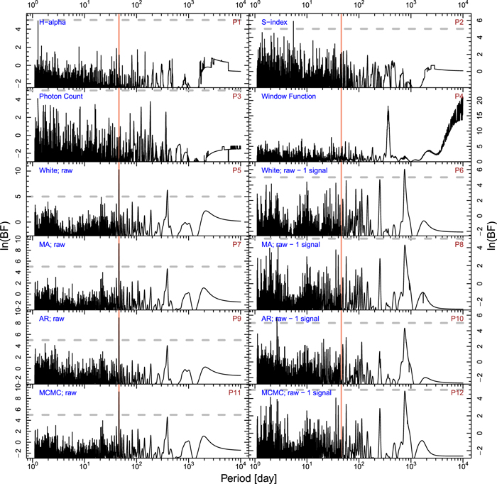
Figure 12. BFPs for HD 64114. The red line shows the signal at a period of 45.8 days.
Download figure:
Standard image High-resolution image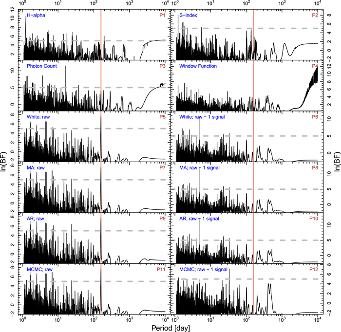
Figure 13. BFPs for HD 8326. The red line shows the signal at a period of 159 days.
Download figure:
Standard image High-resolution image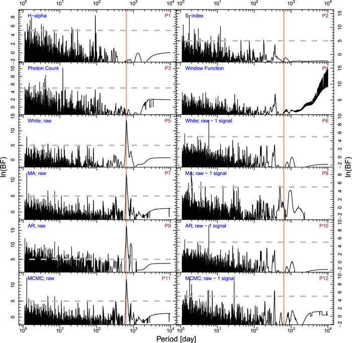
Figure 14. BFPs for HD 164604. The red line shows the signal at a period of 635 days.
Download figure:
Standard image High-resolution image
Figure 15. BFPs for HIP 54373. The red lines show the signals at periods of 15.1 and 7.76 days.
Download figure:
Standard image High-resolution image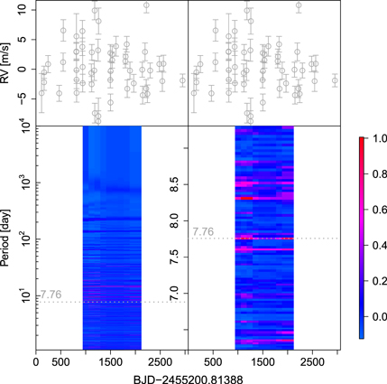
Figure 16. Moving periodogram for HIP 54373 b. The window size is 2000 days and the number of steps is 10. The signal near the 7.76-day signal is its annual alias.
Download figure:
Standard image High-resolution image
Figure 17. Moving periodogram for HIP 54373c. The window size is 2000 days and the number of steps is 10. The signal near the 15.1-day signal is its annual alias.
Download figure:
Standard image High-resolution image
Figure 18. BFPs for HD 24085. The red line shows the signal at a period of 2.05 days.
Download figure:
Standard image High-resolution image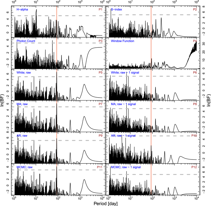
Figure 19. BFPs for HIP 71135. The red line shows the signal at a period of 87.2 days.
Download figure:
Standard image High-resolution image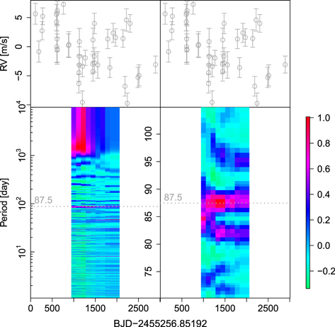
Figure 20. Moving periodogram for HIP 71135 b. The window size is 2000 days and the number of steps is 10. The annual alias of 87.5-day signal also shows excess power in the bottom right panel.
Download figure:
Standard image High-resolution image
5. Conclusion
We introduce a procedure to diagnose the nature of signals in RV data. In this diagnosis framework, we confirm a signal as Keplerian if it is statistically significant, consistent in time, robust in the choice of noise models, and not correlated with stellar activity. We develop an automated algorithm to implement this procedure. The application of this algorithm to the PFS data leads to an initial identification of about 200 primordial signals of high quality.
We report 15 planet candidates from these primordial signals based on analyses of 14 PFS RV data sets that are obtained for six G stars, seven K stars, and one M star. The masses of planets vary from 8 M⊕ to 153 M⊕, and the RV semi-amplitudes vary from 1.7 to 12 m s−1. The detections of these signals demonstrate the ability of PFS to discover small planets around nearby stars.
In particular, we report candidates HD 210193 b, HD 103949 b, HD 8326 b, and HIP 71135 b, which are located in the temperate zones of their stellar hosts and could potentially host temperate moons. We also report candidates HIP 54373 b and c, which form a 1:2 resonance. Such a resonance can stabilize a multiple-planet system for a long period of time, as was discovered in the TRAPPIST-1 system (Gillon et al. 2016; Luger et al. 2017).
Because our algorithm only automatically identifies signals in RV data obtained by a single instrument, we choose to report the signals for targets without other RV data sets available. Thus, we do not check the consistency between PFS and other instruments. An updated algorithm will be developed to automatically analyze multiple RV data sets and to identify potential signals efficiently. Such an algorithm is suitable for modern RV surveys, such as PFS, the High Accuracy Radial Velocity Planet Searcher (HARPS; Pepe et al. 2002), and the Automated Planet Finder (APF; Vogt et al. 2014). Our algorithm also provides a diagnostic framework for reliable detections of exoplanets using the RV method.
This work has made use of data from the European Space Agency (ESA) mission Gaia (https://www.cosmos.esa.int/gaia), processed by the Gaia Data Processing and Analysis Consortium (DPAC, https://www.cosmos.esa.int/web/gaia/dpac/consortium). Funding for the DPAC has been provided by national institutions, in particular the institutions participating in the Gaia Multilateral Agreement. Support for this work was provided by NASA through Hubble Fellowship grant HST-HF2-51399.001 awarded by the Space Telescope Science Institute, which is operated by the Association of Universities for Research in Astronomy, Inc., for NASA, under contract NAS5-26555. The authors acknowledge the years of technical support from LCO staff in the successful operation of PFS, enabling the collection of the data presented in this paper.
Software: R package magicaxis (Robotham 2016), fields (Nychka et al. 2018), minpack.lm (Elzhov et al. 2016).
Footnotes
- *
This paper includes data gathered with the 6.5 m Magellan Telescopes located at the Las Campanas Observatory, Chile.