


Abstract
We present a new grid of presupernova models of massive stars extending in mass between 13 and 120  , covering four metallicities (i.e., [Fe/H] = 0, −1, −2, and −3) and three initial rotation velocities (i.e., 0, 150, and 300 km s−1). The explosion has been simulated following three different assumptions in order to show how the yields depend on the remnant mass−initial mass relation. An extended network from H to Bi is fully coupled to the physical evolution of the models. The main results can be summarized as follows. (a) At solar metallicity, the maximum mass exploding as a red supergiant (RSG) is of the order of 17
  in the nonrotating case, with the more massive stars exploding as Wolf–Rayet (WR) stars. All rotating models, conversely, explode as WR stars. (b) The interplay between the core He-burning and the H-burning shell, triggered by the rotation-induced instabilities, drives the synthesis of a large primary amount of all the products of CNO, not just
  . A fraction of them greatly enriches the radiative part of the He core (and is responsible for the large production of F), and a fraction enters the convective core, leading therefore to an important primary neutron flux able to synthesize heavy nuclei up to Pb. (c) In our scenario, remnant masses of the order of those inferred from the first detections of gravitational waves (GW 150914, GW 151226, GW 170104, GW 170814) are predicted at all metallicities for none or moderate initial rotation velocities.
Export citation and abstract BibTeX RIS
1. Introduction
Massive stars play a pivotal role in the evolution of galaxies because of their influence on the environment: they contribute to the chemical enrichment of the gas clouds, eject an enormous amount of energy either as neutrinos or as kinetic energy, are the protagonists of some of the more spectacular explosions we see in the sky, and leave compact remnants that extend in mass from neutron stars to black holes and are therefore also intimately linked to the spectacular detections of the collapse of compact remnants in binary systems by the LIGO–VIRGO collaboration. A proper understanding of the many evolutionary properties of these stars, including their distribution on the Hertzsprung–Russell (HR) diagram, the relative numbers of stars in the various Wolf–Rayet (WR) stages, the physical and chemical structure of the mantle at the onset of collapse (responsible for the different kinds of core-collapse supernovae), the changes in the surface chemical composition during their evolution, and last but not least, the properties of the explosion including the explosive yields and the mass distribution of the remnants, demands the buildup of an extended and homogeneous grid of models which may be used to study the contribution of these stars to the evolution of galaxies since the formation of the first stars as well as to understand the large variety of objects we observe in the sky. Though extensive literature addressing one aspect or another of the evolution of massive stars exist (Heger et al. 2000; Meynet & Maeder 2003; Heger et al. 2005; Meynet & Maeder 2005; Brott et al. 2011; Limongi & Chieffi 2012; Chieffi & Limongi 2013; Maeder & Meynet 2012; Ekström et al. 2012), a homogeneous and extended set (in mass, metallicity, initial rotation velocity, and number of nuclear species followed) is still missing.
In this paper, we present for the first time all of the relevant properties of a wide set of rotating stellar models: we cover three different initial rotational velocities, namely, v = 0, 150, and 300 km s−1, and four different initial metallicities, namely, [Fe/H] = 0, −1, −2, and −3. The physical and chemical evolution of these models is fully coupled together, and the number of nuclear species followed explicitly amounts to 338, from H to Bi. All of the models were computed with the latest version of our stellar evolution code (FRANEC), improved with respect to the version used in Chieffi & Limongi (2013, CL13 hereinafter) in order to (1) refine the treatment of the angular momentum transport in the envelope of the star, (2) take into account the dynamical mass loss caused by the approach of the luminosity of the star to the Eddington limit, (3) refine the computation of the angular momentum loss due to the stellar wind, and (4) increase the size of the adopted nuclear network. Compared to our previous study, we also adopted a different approach to calibrate the rotation-induced mixing efficiency, which takes advantage now of the observations of the surface chemical composition of many B-stars in the LMC samples of the FLAMES survey (Hunter et al. 2009). This paper is organized as follows: the latest version of the FRANEC code is presented in Section 2, while the calibration of the rotational mixing efficiency is discussed in Section 3. Section 4 is devoted to the presupernova evolution of all the models, while the explosive yields are presented in Section 5. A comparison with models computed by other authors is shown in Section 6, while the remnant mass−initial mass relation is discussed in Section 7. A final summary and the conclusions follow.
2. The Models and the Stellar Evolution Code
The results presented in this paper are based on a grid of models with initial masses 13, 15, 20, 25, 30, 40, 60, 80, and 120 M⊙; initial metallicities [Fe/H] = 0, −1, −2, and −3; and initial equatorial velocities v = 0, 150, and 300 km s−1 (at the beginning of the MS phase). The evolution of all these models has been followed from the pre-main-sequence phase up to the presupernova stage, that is, when the integration of the equations no longer converges. Note that the central temperature of all the models at this stage is well above ∼6  109 K. The evolutions have been computed by means of the latest version of the FRANEC code. The main features of this code, as well as all the input physics and assumptions, have been already extensively discussed in CL13 and are summarized in the Appendix for the sake of completeness. The improvements with respect to the version described in CL13 are the following: (1) better treatment of the angular momentum transport in the envelope of the star, (2) inclusion of the mass loss triggered by the approach to the Eddington limit, (3) proper computation of the angular momentum loss due to the stellar wind, and (4) increase of the size of the adopted nuclear network.
(1) In FRANEC, the star is divided into two zones: the atmosphere and the inner region. In the atmosphere, the luminosity is assumed to be constant so that only three equations, instead of four, are solved. In the presence of rotation, the transport of angular momentum is ignored in the atmosphere, and it is assumed that it rotates as a solid body together with the external border of the inner zone. The mass fraction that we traditionally include in the atmosphere is fixed at 1% of the current total mass of the star, and we adopted this value also in CL13. In order to increase the fraction of mass in which angular momentum is properly transported, we pushed forward the base of the envelope so that in this new grid of models, only 1 part of the mass per 10 thousand is included in the atmosphere, i.e., 99.99% of the mass is now included in the inner zone. Such a choice cannot be maintained for the entire evolution because the dramatic increase of the radius when the star turns redward would imply a prohibitive increase in the number of mesh points and time steps, so we adopted such a refined choice until a star is in central H-burning phase. Beyond that, the border of the inner zone automatically shifts slowly down in mass until it reaches 99% of the current mass. Such a choice is partially justified by the fact that after the core H exhaustion, the star quickly evolves toward the red supergiant (RSG) stage, and therefore, the surface rotation velocity reduces dramatically. (2) During the redward excursion in the HR diagram occurring after core H depletion, the radiative luminosity L = (16πac/3)(GmT4)/(kP)∇ (where ∇ is the local effective temperature gradient, defined as ∇ = d log P/d log T) may approach, and even overcome, the Eddington luminosity L = 4πcGm/k. When this happens, all of the zones above the region exceeding this limit become essentially unbound, and one would expect a strong episode of mass loss. In order to treat such a phenomenon, we remove all of the unbound zones with a maximum limit of 3  10−3 M⊙ lost per model. (3) When a star loses mass, it also loses a certain amount of angular momentum. The determination of this amount is not trivial; it is subject to large uncertainties and is somewhat arbitrary. In CL13, we arbitrarily made a minimalist choice in the sense that the amount of angular momentum removed per time step was simply the one contained in the mass removed by the star as a consequence of mass loss. In the present calculations, on the contrary, we explicitly compute the angular momentum loss J (
 , where jsurf is the specific angular momentum at the surface and
  and dt the mass-loss rate and the time step, respectively) and remove such an amount from the outer region of the star by requiring that no more than a few per cent of the angular momentum may be removed from each layer. (4) The nuclear network adopted in CL13 included 293 isotopes, from H to
  , coupled by all possible links among them due to weak and strong interactions, for a total of about 3000 reactions in the various nuclear-burning stages. Since one of the main issue related to the nucleosynthesis in rotating massive stars of low metallicity is the production of the s-process elements (see below), we extend our nuclear network in order to include as many elements as possible between
  and
and  . In order to save computer memory and computational time, we make the following assumption. Since in the neutron capture chain the slowest reactions are the ones involving magic nuclei, we explicitly follow, and include into the nuclear network, all of the stable and unstable isotopes around the magic numbers corresponding to N = 82 and N = 126, consider for these isotopes only neutron captures and beta decays, and assume all of the other intermediate isotopes at the local equilibrium. In this way we are able to follow in detail the flux of neutrons through all of the magic number bottlenecks. As a consequence, the nuclear network adopted in the present calculations includes 335 isotopes (from neutrons to
  ) and is reported in Table 1.
Table 1. Nuclear Network Adopted in the Present Calculations
| Element | Amin | Amax | Element | Amin | Amax |
|---|---|---|---|---|---|
| n | 1 | 1 | Co | 54 | 61 |
| H | 1 | 3 | Ni | 56 | 65 |
| He | 3 | 4 | Cu | 57 | 66 |
| Li | 6 | 7 | Zn | 60 | 71 |
| Be | 7 | 10 | Ga | 62 | 72 |
| B | 10 | 11 | Ge | 64 | 77 |
| C | 12 | 14 | As | 71 | 77 |
| N | 13 | 16 | Se | 74 | 83 |
| O | 15 | 19 | Br | 75 | 83 |
| F | 17 | 20 | Kr | 78 | 87 |
| Ne | 20 | 23 | Rb | 79 | 88 |
| Na | 21 | 24 | Sr | 84 | 91 |
| Mg | 23 | 27 | Y | 85 | 91 |
| Al | 25 | 28 | Zr | 90 | 97 |
| Si | 27 | 32 | Nb | 91 | 97 |
| P | 29 | 34 | Mo | 92 | 98 |
| S | 31 | 37 | Xe | 132 | 135 |
| Cl | 33 | 38 | Cs | 133 | 138 |
| Ar | 36 | 41 | Ba | 134 | 139 |
| K | 37 | 42 | La | 138 | 140 |
| Ca | 40 | 49 | Ce | 140 | 141 |
| Sc | 41 | 49 | Pr | 141 | 142 |
| Ti | 44 | 51 | Nd | 142 | 144 |
| V | 45 | 52 | Hg | 202 | 205 |
| Cr | 48 | 55 | Tl | 203 | 206 |
| Mn | 50 | 57 | Pb | 204 | 209 |
| Fe | 52 | 61 | Bi | 208 | 209 |
Download table as: ASCIITypeset image
In order to check the reliability of this assumption, we performed a one-zone calculation of a typical core He burning with two different nuclear networks, the one reported in Table 1 and another one in which we also added all of the stable isotopes between  and
and  (Table 2). This test was done by using the temporal evolution of the central temperature and density obtained for a 20 M⊙ star having [Fe/H] = −3 and initial equatorial velocity v = 300 km s−1. The continuous ingestion of fresh
  (driven by rotation-induced mixing; see below) that powers a steady production of primary neutrons is simulated by keeping constant the neutron mass fraction during the evolution: more specifically, the neutron density is set equal to a mass fraction of 10−20 (i.e., the value corresponding to the starting model; see below) at the beginning of each time step . The computation starts when
  (α, n) begins to be efficient, which in this specific case pertains to when the central He mass fraction drops to ∼0.08 and ends at the central He-exhaustion stage. The result of this test clearly shows that at the end of the central He burning, both runs similarly populate the region 131 < A < 145 (i.e., around the magic neutron closure shell n = 82). Figure 1 shows in fact that the final abundances of these nuclei vary between 20% and 40%. Figure 2 shows the temporal evolution of
  obtained in the two runs: the red line refers to the reference network shown in Table 1 while the black line refers to the more extended network that also includes the elements reported in Table 2. Both of these plots show that our approximation does not alter substantially the flux of the matter through the neutron magic number bottlenecks because the increase of the abundances of the heavy elements induced by rotation is an order of magnitude larger than the differences found above by comparing the two networks.

Figure 1. Variation between the abundances obtained with our reference network (Table 1), Xref, and the ones obtained with the larger network, Xfull, i.e., also including in the reference network the isotopes reported in Table 2.
Download figure:
Standard image High-resolution image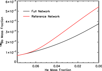
Figure 2. Evolution of the 138Ba mass fraction as a function of the 4He mass fraction in the one-zone model calculation. The black line is obtained with the network in Table 1, while the red line is obtained with the network in Table 2 (see text).
Download figure:
Standard image High-resolution imageTable 2. Isotopes Included between 98Mo and 132Xe in the One-zone He-burning Calculation
| Element | Amin | Amax |
|---|---|---|
| Tc | 99 | 99 |
| Ru | 100 | 102 |
| Rh | 103 | 103 |
| Pd | 104 | 104 |
| Ag | 109 | 109 |
| Cd | 110 | 114 |
| In | 115 | 115 |
| Sn | 116 | 120 |
| Sb | 121 | 121 |
| Te | 122 | 126 |
| I | 127 | 127 |
Download table as: ASCIITypeset image
The nuclear cross-sections and the weak interaction rates have been updated, whenever possible, with respect to the ones adopted in our previous version of the code. Most of them have been extracted from the STARLIB database (Sallaska et al. 2013). Tables 3 and 4 show the full reference matrix of all the processes taken into account in the network, together with its proper legend. As usual, for the weak interaction rates, β+ and β− mean the sum of both the electron capture and the β+ decay and the positron capture and the β− decay, respectively.
Table 3. Network Reference Matrix
| Isotope | (p, α) | (p, n) | (p, γ) | (α, p) | (α, n) | (α, γ) | (n, p) | (n, α) | (n, γ) | (γ, p) | (γ, α) | (γ, n) | (β+) | (β−) |
|---|---|---|---|---|---|---|---|---|---|---|---|---|---|---|
| 2H | desc | nacr | ka03 | |||||||||||
| 3H | desc | cf88 | rath | |||||||||||
| 3He | bet+ | desc | ka03 | |||||||||||
| 6Li | nacr | nacr | cf88 | mafo | ||||||||||
| 7Li | desc | desc | wago | cf88 | nacr | ka03 | ||||||||
| 7Be | nacr | nacr | nacr | desc | wago | cf88 | ||||||||
| 9Be | nacr | nacr | wago | nacr | ka03 | |||||||||
| 10Be | wago | wago | fkth | fkth | bb92 | rath | ||||||||
| 10B | nacr | nacr | wago | cf88 | cf88 | wies | ||||||||
| 11B | nacr | bb92 | bb92 | bb92 | bb92 | |||||||||
| 12C | nacr | nacr | cf88 | ku02 | nacr | ka03 | ||||||||
| 13C | wago | cf88 | nacr | wago | nacr | fkth | ka03 | ka03 |
Notes. bet+: beta plus decay, desc: Descouvemont et al. (2004), ka03: Dillmann et al. (2009), KADoNiS v0.3, nacr: Angulo et al. (1999), NACRE, cf88: Caughlan & Fowler (1988), ku02: Kunz et al. (2002), adopted rate, im05: Imbriani et al. (2005), mc10: Iliadis et al. (2010), bb92: Rauscher et al. (1994), wies: M. Wiescher and collaborators, rath: last version of REACLIB available at the Web site https://nucastro.org/reaclib.html, wago: Wagoner (1969), mafo: Malaney & Fowler (1989), fkth: Cowan et al. (1991), wfho: Wagoner et al. (1967), od94: Oda et al. (1994), bl03: Blackmon et al. (2003), kart: Dillmann et al. (2009) in the energy range 5–100 keV and Rauscher & Thielemann (2000) above this limit, but rescaled to match the experimental values of Dillmann et al. (2009) at 100 keV, mc11: Sallaska et al. (2011), rt: Rauscher & Thielemann (2000), de07: de Smet et al. (2007), ko97: Koehler et al. (1997), ffn8: Fuller et al. (1982), og10: Oginni et al. (2011), ka02: Dillmann et al. (2006), KADoNiS v0.2, il09: Iliadis et al. (2011), nass: Nassar et al. (2006), lp00: Langanke & Martínez-Pinedo (2000), laur: van Wormer et al. (1994), re98: Rehm et al. (1998), taka: Takahashi & Yokoi (1987), tanu: terrestrial half-life.
aWe treat the ground (26Alg) and isomeric (26Alm) states of 26Al as separate species for T ≤ 109 K, while we assume the two states to be in statistical equilibrium (and therefore we consider just one isotope) above this temperature (Limongi & Chieffi 2006). b26Alg ground state. c26Alm isomeric state.Only a portion of this table is shown here to demonstrate its form and content. A machine-readable version of the full table is available.
Download table as: DataTypeset image
Table 4. Network Reference Matrix for Special Nuclear Reactions
| Reaction | References |
|---|---|
| p (p, e+ν)2H | nacr |
| 3He (3He, 2p)α | nacr |
| α (3He, γ)7Be | cy08 |
| 2H (2H, p)3H | nacr |
| 2H (2H, n)3He | desc |
| 2H (2H, γ)α | nacr |
| 3H (p, 2H)2H | nacr |
| 3H (2H, n)α | desc |
| 3He (2H, p)α | desc |
| 3He (3H, 2H)α | cf88 |
| 3He (n, 2H)2H | desc |
| 2α (α, γ)12C | nacr |
| α (p, 2H)3He | desc |
| α (2H, 3H)3He | cf88 |
| α (3H, n)6Li | cf88 |
| α (3H, n)6Li | desc |
| α (3He, p)6Li | nacr |
| α (n, 2H)3H | desc |
| 6Li (p, 3He)α | nacr |
| 6Li (2H, n)7Be | mafo |
| 6Li (2H, p)7Li | mafo |
| 6Li (n, 3H)α | cf88 |
| 7Li (p, 2H)6Li | mafo |
| 7Li (2H, p)8Li | mafo |
| 7Li (3H, n)9Be | bb92 |
| 7Be (n, 2H)6Li | mafo |
| 9Be (3H, n)11B | bb92 |
| 9Be (n, 2H)8Li | mafo |
| 9Be (n, 3H)7Li | bb92 |
| 11B (n, 3H)9Be | bb92 |
| 13C (2H, n)14N | bb92 |
| 14C (2H, n)15N | bb92 |
| 14N (n, 2H)13C | bb92 |
| 15N (n, 2H)14C | bb92 |
| 12C (12C, n)23Mg | da77 |
| 12C (12C, p)23Na | cf88 |
| 12C (12C, α)20Ne | cf88 |
| 12C (16O, n)27Si | cf88 |
| 12C (16O, p)27Al | cf88 |
| 12C (16O, α)24Mg | cf88 |
| 16O (16O, n)31S | cf88 |
| 16O (16O, p)31P | cf88 |
| 16O (16O, α)28Si | cf88 |
| 20Ne (12C, n)31S | rolf |
| 20Ne (12C, p)31P | rolf |
| 20Ne (12C, α)28Si | rolf |
Note. cy08: Cyburt & Davids (2008), da77: Dayras et al. (1977), rolf: C. Rolfs and collaborators.
Download table as: ASCIITypeset image
The initial composition adopted for the solar metallicity models is the one provided by Asplund et al. (2009), which corresponds to a total metallicity Z = 1.345  10−2. For the models with initial metallicity lower than solar, we assume the same scaled solar distribution for all elements, with the exception of C, O, Mg, Si, S, Ar, Ca, and Ti, for which we adopt an enhancement with respect to Fe derived from the observations of low-metallicity stars, i.e., [C/Fe] = 0.18, [O/Fe] = 0.47, [Mg/Fe] = 0.0.27, [Si/Fe] = 0.37, [S/Fe] = 0.35, [Ar/Fe] = 0.35, [Ca/Fe] = 0.33, and [Ti/Fe] = 0.23 (Cayrel et al. 2004; Spite et al. 2005). As a result of these enhancements, the total metallicity corresponding to [Fe/H] = −1, −2, and −3 is Z = 3.236
  10−3, 3.236
  10−4, and 3.236
  10−5, respectively. The initial He abundances adopted at the various metallicities are 0.265 ([Fe/H] = 0), 0.25 ([Fe/H] = −1), and 0.24 ([Fe/H] = −2 and [Fe/H] = −3). By the way, we remind the reader that the abundance ratio [X/Y] is defined as [X/Y] = log(X/Y)–log(X/Y)⊙.
3. Calibration of the Mixing Efficiency
Since rotation is a multidimensional physical phenomenon, its inclusion in a 1D stellar evolution code implies a certain number of assumptions (Maeder & Meynet 2000, CL13). Therefore, the calculation of the diffusion coefficients adopted to transport both the angular momentum and the chemical composition (see the Appendix) is intrinsically uncertain. For this reason, the efficiency of the rotation-induced mixing must be calibrated in some way. Different authors adopt different techniques to perform such a calibration, e.g., Heger et al. (2000) require a surface enrichment of N of the order of 2–3 in solar metallicity models with initial mass in the range 10–20 M⊙, while Brott et al. (2011) try to reproduce the observed N abundance as a function of the projected rotation velocity (the Hunter diagram hereafter) in the LMC samples of the FLAMES survey (Hunter et al. 2009). In CL13, we computed only solar-metallicity models, and therefore, we followed the same idea as Heger et al. (2000). In general, since we have two free parameters, namely fc and fμ (Heger et al. 2000, CL13), and only one requirement, we cannot determine a single solution to this problem, only a family of possible choices. For this reason, in CL13, we chose a conservative approach by fixing fc = 1.0 and by calibrating fμ in order to obtain an enhancement of the surface N abundance by a factor of 2–3 in a 20 M⊙ star of solar metallicity at core H depletion. As a result of that calibration, we found that the best choice of the two mixing parameters was fc = 1.0 and fμ = 0.03. In this paper, we present models of various metallicities, and hence we decided to check whether the calibration obtained in CL13 is valid at subsolar metallicities. For this reason, we considered the LMC samples of the FLAMES survey that are centered on the clusters NGC 2004 and N11 (Hunter et al. 2008). The number of core H-burning stars (log g ≥ 3.2), for which the determination of both the surface N abundance and v sin (i) is available, is 62 and 30 for NGC 2004 and N11, respectively. Therefore, to obtain a sample that is as homogeneous and populated as possible, we decide to use only NGC 2004.
Figure 3 shows a plot of the surface N abundance as a function of the projected rotational velocity for the sample of stars in NGC 2004. While there are stars that follow the general trend one would expect from the rotation-induced mixing (i.e., the higher the initial rotation velocity, the higher the surface N enhancement), there is also a conspicuous number of stars that do not follow such a general expectation: we will ignore these stars in the present calibration. We followed the same procedure adopted by Brott et al. (2011), i.e., we aimed to reproduce what we expect should be the main trend of the surface N enhancement as a function of the rotation velocity. The typical mass estimated for this sample is ∼13 M⊙; therefore, we computed a series of models of 13 M⊙ and different initial equatorial rotation velocities, assuming fc = 1.0 and fμ = 0.03. The adopted initial metallicity is [Fe/H] = −0.45, and the abundances of most of the elements are assumed to be scaled solar, with the exceptions of C, N, O, Mg, and Si, for which we adopt the same scaling reported by Brott et al. (2011) in their Table 1. Figure 3 shows the evolutionary tracks of these models (green dotted lines) superimposed on the observed data. Note that the theoretical velocities have been multiplied by π/4 in order to take into account the random inclination of the rotational axis. The figure shows that the mixing obtained with fc = 1.0 and fμ = 0.03 is not efficient enough to explain the highest N abundances observed for the fastest rotating models. Therefore, we modified the two coefficients, trying to get close to these highly enhanced stars. After a series of tests, we decided (arbitrarily) to adopt fc = 1.5 and fμ = 0.01. Figure 3 shows the evolutionary tracks computed with these choices as red dotted lines. The red and green solid lines are obtained by connecting the position of the various models at the central H exhaustion. As a final comment, let us remark that with the present choices of fc and fμ, the surface N enhancement obtained in a 20 M⊙ star of solar metallicity at core H depletion is of the order of 5–6, i.e., not much higher than the value obtained in CL13.

Figure 3. Surface N abundance (black dots) as a function of the projected rotation velocity for a sample of stars in the LMC cluster NCG 2004 (Hunter et al. 2008). Evolutionary tracks of a 13 M⊙ star with different initial rotation velocities, computed with two different calibrations of the rotation-driven mixing efficiency, namely fc = 1.0 and fμ = 0.03 (green line), and fc = 1.5 and fμ = 0.01 (red lines).
Download figure:
Standard image High-resolution image4. Presupernova Evolutions
We have already discussed extensively in CL13 the influence of rotation (see also Heger et al. 2000; Meynet & Maeder 2000), and of the associated instabilities, on the evolution of a generation of massive stars of solar metallicity and initial rotation velocity v = 300 km s−1. Here we discuss the influence of the metallicity and two different initial equatorial velocities (150 and 300 km s−1) on the evolution of a generation of massive stars. It is very important to note, and as a reminder throughout the reading of this paper, that the role of rotation as a function of mass largely depends on the way in which each grid of models is computed. More specifically, the dependence of any property (connected to rotation) on the mass is completely different if one compares models having the same initial rotation velocity or, e.g., the same fraction of break-out velocity. The reason is that the impact of rotation on the evolution of a star roughly scales directly with  , but this parameter scales inversely with the mass if the initial rotation velocity is kept constant (Figure 4). Hence, a set of models of different masses and the same initial rotation velocity will obviously show a progressive reduction of the rotation-induced effects as the initial mass increases. Note, also, that the setup of the stellar evolution code adopted for the present computations is different from the one adopted in CL13; therefore, the solar-metallicity models presented here are not identical to those discussed in that paper.
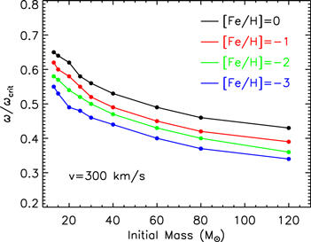
Figure 4. Ratio between the angular and the critical velocities at the beginning of the main sequence for all models of the present grid.
Download figure:
Standard image High-resolution imageTable 5 summarizes the main evolutionary properties of all the computed models in the present grid, at the end of the main nuclear-burning stages (e.g., "MS" refers to the end of the pre-main-sequence phase, "H" to the end of the core H-burning phase, "He" to the end of the core He-burning phase, "PSN" to the end of the evolution). For each burning stage, the various columns in this table have the following meaning: (column 1) the evolutionary stage (as mentioned above), (column 2) the star's lifetime in years, (column 3) the maximum extension of the convective core in solar masses, (column 4) the logarithm of the effective temperature in Kelvin, (column 5) the logarithm of the luminosity in solar luminosities, (column 6) the total mass of the star in solar masses, (column 7) the He core mass in solar masses, (column 8) the CO core mass in solar masses, (column 9) the equatorial velocity in km s−1, (column 10) the surface angular velocity in s−1, (column 11) the ratio between the surface and the critical angular velocity, (column 12) the total stellar angular momentum in units of 1053 g cm2 s−1, (columns 13 to 15) the surface H, He, and N mass fractions, and (columns 16 to 17) the N/C and N/O number ratios.
Table 5. Main Evolutionary Properties of the Models with v = 000 km s−1 and Metallicity [Fe/H] = 0
| Phase | Time | MCC | log(Teff) | log(L/L⊙) | M | M*He | MCO | vequa | ωsup | ω/ωcrit | Jtot | Hsup | Hesup | Nsup | N/C | N/O |
|---|---|---|---|---|---|---|---|---|---|---|---|---|---|---|---|---|
| (years) | (M⊙) | (K) | (M⊙) | (M⊙) | (M⊙) | (km s−1) | (s−1) | 1053 | Mass | Mass | Mass | Number | Number | |||
| g cm2 s−1 | Fraction | Fraction | Fraction | Ratio | Ratio | |||||||||||
| 13 | ||||||||||||||||
| MS | 1.36(+5) | 0.00 | 4.47 | 4.08 | 13.00 | 0.00 | 0.00 | 0.00(+0) | 0.00(+00) | 0.00(+0) | 0.00(+0) | 7.21(−1) | 2.65(−1) | 6.95(−4) | 2.96(−1) | 1.21(−1) |
| H | 1.61(+7) | 5.47 | 4.39 | 4.53 | 12.90 | 2.95 | 0.00 | 0.00(+0) | 0.00(+00) | 0.00(+0) | 0.00(+0) | 7.21(−1) | 2.65(−1) | 6.95(−4) | 2.96(−1) | 1.21(−1) |
| He | 1.09(+6) | 1.70 | 3.57 | 4.70 | 12.10 | 4.08 | 1.74 | 0.00(+0) | 0.00(+00) | 0.00(+0) | 0.00(+0) | 7.02(−1) | 2.85(−1) | 2.31(−3) | 1.60(+0) | 4.57(−1) |
| C | 9.09(+3) | 0.60 | 3.55 | 4.82 | 11.90 | 4.08 | 1.97 | 0.00(+0) | 0.00(+00) | 0.00(+0) | 0.00(+0) | 7.02(−1) | 2.85(−1) | 2.31(−3) | 1.61(+0) | 4.57(−1) |
| Ne | 5.68(+0) | 0.56 | 3.55 | 4.82 | 11.90 | 4.08 | 2.03 | 0.00(+0) | 0.00(+00) | 0.00(+0) | 0.00(+0) | 7.02(−1) | 2.85(−1) | 2.31(−3) | 1.61(+0) | 4.57(−1) |
| O | 4.17(+0) | 0.93 | 3.55 | 4.82 | 11.90 | 4.08 | 2.03 | 0.00(+0) | 0.00(+00) | 0.00(+0) | 0.00(+0) | 7.02(−1) | 2.85(−1) | 2.31(−3) | 1.61(+0) | 4.57(−1) |
| Si | 3.50(−1) | 1.09 | 3.55 | 4.82 | 11.90 | 4.08 | 2.03 | 0.00(+0) | 0.00(+00) | 0.00(+0) | 0.00(+0) | 7.02(−1) | 2.85(−1) | 2.31(−3) | 1.61(+0) | 4.57(−1) |
| PSN | 1.77(−3) | 0.00 | 3.55 | 4.82 | 11.90 | 4.08 | 2.03 | 0.00(+0) | 0.00(+00) | 0.00(+0) | 0.00(+0) | 7.02(−1) | 2.85(−1) | 2.31(−3) | 1.61(+0) | 4.57(−1) |
*MHe = 0 means that the star has lost the whole H rich envelope and has become a bare He core.
Only a portion of this table is shown here to demonstrate its form and content. A machine-readable version of the full table is available.
Download table as: DataTypeset image
4.1. Core H Burning
Mass loss significantly affects the evolution of a massive star in the central H-burning phase, and its influence increases with the initial mass because of the large dependence of the mass-loss rate on the luminosity (Vink et al. 2000, 2001). With the currently adopted mass-loss prescriptions, nonrotating solar-metallicity models with initial mass larger than 60 M⊙ lose a substantial fraction of their H-rich envelope, and therefore enter the WR stage already in this phase. In particular, they become WNL stars during the late stages of core H burning. Note, however, that the minimum mass that becomes a WR star does not depend only on the adopted mass-loss rate but also on other uncertain properties like, e.g., the size of the H convective core. In fact, as it is well known, the inclusion of some amount of convective core overshooting makes the evolutionary tracks cooler and brighter compared to the standard ones. This implies an overall higher mass loss and therefore a reduction of the minimum mass entering the WR stage.
Table 6 shows the lifetimes during the various WR stages (see Chieffi & Limongi 2013 for the definition of the various WR stages). In particular, the following quantities are reported: the initial mass (column 1), the lifetime during the O-type phase in years (column 2), the total WR lifetime in years (column 3), the lifetime during the WNL phase in years (column 4), the H or He central mass fraction at the time the star enters the WNL stage (column 5), the lifetime during the WNE phase in years (column 6), the H or He central mass fraction at the time the star enters the WNE stage (column 7), the lifetime during the WNC phase in years (column 8), the H or He central mass fraction at the time the star enters the WNC stage (column 9), the lifetime during the WC phase in years (column 10), and the H or He central mass fraction at the time the star enters the WC stage (column 11).
Table 6. Wolf–Rayet Lifetimes of the Models with v = 0 km s−1 and Metallicity [Fe/H] = 0
| Initial Mass | tO | tWR | tWNL | Hc/Hec (WNL) | tWNE | Hc/Hec (WNE) | tWNC | Hc/Hec (WNC) | tWC | Hc/Hec (WC) |
|---|---|---|---|---|---|---|---|---|---|---|
| (M⊙) | (years) | (years) | (years) | Mass Fraction | (years) | Mass Fraction | (years) | Mass Fraction | (years) | Mass Fraction |
| 13 | ||||||||||
| 15 | 8.31(+4) | |||||||||
| 20 | 6.44(+6) | 7.79(+4) | 7.79(+4) | He(0.05) | ||||||
| 25 | 5.94(+6) | 2.89(+5) | 1.51(+5) | He(0.45) | 1.39(+5) | He(0.14) | ||||
| 30 | 5.14(+6) | 3.07(+5) | 2.07(+5) | He(0.57) | 1.00(+5) | He(0.11) | ||||
| 40 | 4.24(+6) | 3.03(+5) | 1.75(+5) | He(0.73) | 1.28(+5) | He(0.20) | ||||
| 60 | 3.20(+6) | 3.52(+5) | 7.69(+4) | He(0.96) | 1.56(+5) | He(0.67) | 1.67(+4) | He(0.20) | 1.03(+5) | He(0.16) |
| 80 | 2.63(+6) | 3.71(+5) | 9.27(+4) | H (0.01) | 1.01(+5) | He(0.78) | 1.61(+4) | He(0.40) | 1.61(+5) | He(0.34) |
| 120 | 2.17(+6) | 5.46(+5) | 2.65(+5) | H (0.09) | 6.63(+4) | He(0.86) | 8.40(+3) | He(0.58) | 2.06(+5) | He(0.55) |
Only a portion of this table is shown here to demonstrate its form and content. A machine-readable version of the full table is available.
Download table as: DataTypeset image
The He core mass (MHe) at core H exhaustion increases, in general, with the initial mass (Mini) because it scales with the size of the H convective core that, in turn, increases with the mass of the star. Figure 5 shows the MHe–Mini (red dashed line) and the Mtot–Mini (blue dashed line) relations at core H depletion, Mtot being the actual mass of the star. The bending of the MHe–Mini relation is a consequence of the tremendous mass loss experienced by the more massive stars.

Figure 5. Total mass (blue solid line) and He core mass (red solid line) at core H exhaustion as a function of the initial mass for nonrotating, solar-metallicity models. The label "WNL" marks the models entering the Wolf–Rayet stage.
Download figure:
Standard image High-resolution imageAs the metallicity decreases, mass loss reduces significantly because it scales as  (Vink et al. 2000, 2001). As a consequence, all nonrotating models with [Fe/H] ≤ −1 evolve essentially at constant mass in this phase. A lower initial metallicity also implies a reduction of the total abundance of the CNO nuclei, and therefore an increase of the core H-burning temperature. This leads, in principle, to more extended convective cores and hence to larger MHe at core H depletion (Tornambe' & Chieffi 1986). However, this effect is largely mitigated in our models by the inclusion of 0.2HP of overshooting during the central H-burning phase (HP = −d log r/d log P), an occurrence that washes out most of the dependence of the convective core, and hence of the MHe, on the initial metallicity. Figure 6 shows, in fact, that stars with initial mass M < 40 M⊙ develop He core masses essentially independent of the initial metallicity. Stars above this limiting mass show sizable differences between models with solar and nonsolar metallicities, but these differences are just the indirect effect of mass loss, as we have already discussed above.
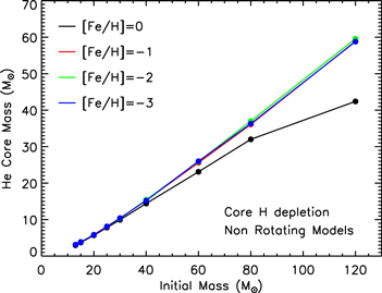
Figure 6. He core mass at core H depletion as a function of the initial mass for nonrotating models at various metallicities.
Download figure:
Standard image High-resolution imageThe effect of rotation on the evolutionary path of a massive star in the HR diagram in the central H-burning phase is twofold (Maeder & Meynet 2000, 2001, 2012; Meynet & Maeder 2000, CL13). On one hand, the lower gravity, due to the combined effects of the centrifugal force and the angular momentum transport, pushes the star toward lower effective temperatures. On the other hand, the increase of the mean molecular weight in the radiative envelope, due to rotationally driven mixing, has two key consequences: (a) the mass of the H convective core increases, making therefore the track brighter and cooler (like the effect of the convective core overshooting), and (b) the opacity in the H-rich mantle decreases, making the star more luminous and more compact, and favoring therefore a blueward evolution. Depending on the initial mass, initial metallicity, and initial rotation velocity, one of these effects may prevail over the others. Figure 7 shows that, during the core H-burning phase, the evolutionary tracks of rotating solar-metallicity stars are, on average, brighter and hotter than those of the nonrotating ones and hence the increase of the mean molecular weight in the H-rich mantle is the dominant effect. On the contrary, as the metallicity decreases, the evolutionary tracks of rotating stars become brighter and cooler than those of the nonrotating ones, and hence the reduction of the effective gravity, due to the centrifugal force and the angular momentum transport, mainly controls the evolution.
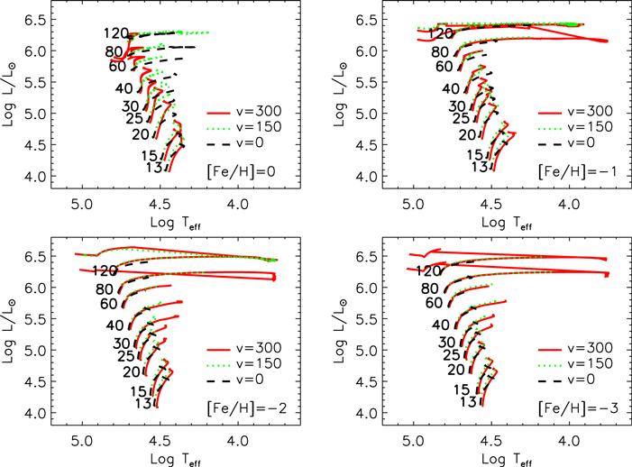
Figure 7. Evolutionary tracks in the HR diagram of all the computed models during the core H-burning phase at various metallicities. Black dashed lines refer to nonrotating models, and green dotted and red lines to models with initial velocity v = 150 km s−1 and v = 300 km s−1, respectively.
Download figure:
Standard image High-resolution imageA change in the evolutionary path of a star in the HR diagram obviously affects the mass-loss rate. At solar metallicity, the amount of mass lost during the H-burning phase increases significantly with the initial rotation velocity. As a consequence, the minimum mass entering the WNL stage in this phase decreases from M > 60 M⊙ in the nonrotating models to M > 40 M⊙ in the rotating ones (Table 6). At subsolar metallicities, conversely, the effect of rotation on the mass-loss rate is negligible because of its steep dependence on the metallicity. Hence, at subsolar metallicities, the rotating models also evolve essentially at constant mass, with the exception of the two most massive ones. These models experience a pronounced redward excursion in the HR diagram, approach the Eddington limit (when the effective temperature drops below log Teff ∼ 3.9), enter a phase of very high mass loss that drives the ejection of a substantial fraction of their H-rich envelope, and eventually become WNL stars (Figure 7). Thus, in general, the minimum mass entering the WNL stage during the core H-burning phase decreases with increasing metallicity and with increasing initial rotational velocity (see Table 6).
In the absence of rotation, the mixing of matter occurs only within regions where thermal instabilities (convection) grow. By contrast, in the presence of rotation, additional mixing also occurs in thermally stable (radiative) regions. The two main engines that drive such a mixing are the meridional circulation and the secular shear. The former instability dominates the diffusion of the chemical composition in the inner part of the radiative mantle, i.e., close to the outer edge of the H convective core, while the secular shear controls the mixing in the outer layers (see, e.g., Figure 5 in Chieffi & Limongi 2013). The main consequences of this rotation-driven mixing are (1) the increase of the core H-burning lifetime, (2) the increase of the He core mass at core H exhaustion, and (3) the surface enhancement of the  abundance.
Figure 8 shows the effect of the rotation-induced mixing on the size of the He core at core H depletion as a function of the initial rotation velocity, for the various metallicities. The general trend is that, for any fixed initial mass, the higher the initial rotation velocity, the greater the MHe at core H depletion. This general trend fails for those models in which mass loss is efficient enough to reduce substantially the total mass of the star, in particular for the fast rotating solar-metallicity models with M > 40 M⊙ as well as the fast rotating ones with [Fe/H] = −1 and mass M > 60 M⊙. Figure 9 shows the effect of the metallicity on the size of MHe at core H depletion, for a fixed initial rotation velocity. It is worth noting that stars with initial mass M < 25 M⊙ do not show a significant dependence of the MHe on the initial metallicity (at least in the range of initial rotational velocities studied in this paper). More massive stars, conversely, show an increase in MHe as the metallicity decreases (for both rotational velocities) because the lack of large mass loss allows these stars to retain to the end of the H-burning phase a convective core bigger than that present in stars that have lost a consistent amount of mass.
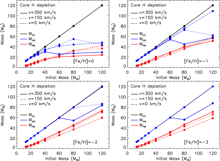
Figure 8. Total mass (blue lines) and He core mass (red lines) at core H depletion as a function of the initial mass for various metallicities and different initial rotation velocities, i.e., v = 0 km s−1 (dashed lines), v = 150 km s−1 (dotted lines), and v = 300 km s−1 solid lines.
Download figure:
Standard image High-resolution image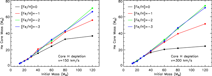
Figure 9. He core mass at core H depletion as a function of the initial mass at various metallicities for models with initial rotation velocities v = 150 km s−1 (left panel) and v = 300 km s−1 (right panel).
Download figure:
Standard image High-resolution imageAn important aspect of rotating models that is worth discussing is the temporal variation of the surface chemical composition during the main-sequence phase. Figures 10 and 11 show the effect of metallicity on the trend of the surface  abundance versus the current equatorial rotational velocity during the core H-burning phase (the so-called Hunter diagram). At solar metallicity, most of the stars show a quite smooth increase in the surface
  abundance coupled to a corresponding decrease in the surface equatorial rotational velocity. This behavior is the consequence of the efficient loss of angular momentum triggered by the strong stellar winds. The only exceptions to this behavior are the two smaller masses, namely the 13 M⊙ and the 15 M⊙, that show an increase in
  at almost constant equatorial rotational velocities because of the modest loss of angular momentum from the surface due to the weaker stellar wind.

Figure 10. Ratio between the surface N abundance and the initial one as a function of the equatorial velocity during the core H-burning phase for solar-metallicity rotating models. The dots with different colors mark the locations corresponding to a given percentage of the total H-burning lifetime (see the legend in the figure corresponding to the 20 M⊙ star model).
Download figure:
Standard image High-resolution image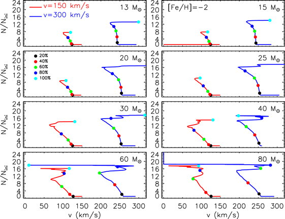
Figure 11. Same as Figure 10 but for metallicity [Fe/H] = −2.
Download figure:
Standard image High-resolution imageLow-metallicity models behave essentially like the 13 and 15 M⊙ stars with solar metallicity. In fact, due to the strong reduction in mass loss with metallicity, in this case the increase of the surface  is coupled to a modest reduction of the surface equatorial velocity; a substantial change of the surface velocity occurs only toward the end of the H-burning phase, when the surface abundance of
  no longer changes. It goes without saying that these different behaviors may play a crucial role in the interpretation of the Hunter diagrams. A more detailed study of this issue will be addressed in a forthcoming paper.
Another key feature worth discussing is the variation of the total angular momentum and its internal distribution at the end of the core H-burning phase. Both of these properties are the result of the combined effects of the transport and the loss of angular momentum. The current solar-metallicity models lose between ∼30% and ∼90% of their initial angular momentum during the core H-burning phase (see Figure 12). The solid black and red lines show the internal (cumulative) run of the angular momentum at H ignition and exhaustion, respectively, for both 15 and the 60  . As expected, the larger the mass and the larger the initial equatorial velocity, the more efficient the angular momentum loss. The red dashed lines in the same figure show the run of the (cumulative) change (with respect to the H ignition) of angular momentum (in per cent) at the central H-exhaustion phase. A comparison between the two red dashed lines in the left panels (which refer to 15
  ) shows that the amount of angular momentum lost by the H-exhausted core is almost independent of the initial rotation velocity. This is easily understood by remembering that in the convective zones, we assume a flat omega profile, which implies the maximum possible transport of angular momentum. Also, the 60
  star with v = 150 km s−1 behaves similarly to the two 15
  stars, while the 60
  star rotating initially at 300 km s−1 shows a much more pronounced reduction of angular momentum in the H-exhausted core. This is due to the very efficient mass loss that this star experiences in the H-burning phase. At lower metallicities, the large decrease in the stellar wind inhibits the loss of angular momentum; as a consequence, these models do not lose a substantial amount of angular momentum (see Figure 13). Note, however, that also in this case the presence of a convective core forces the angular momentum present in the H-exhausted core to drop by an amount quite similar to that lost by the more metal-rich stars.
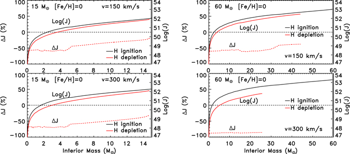
Figure 12. Total (cumulative) angular momentum (J) at the core H-ignition (black solid line) and core H-depletion (red solid line) phases as a function of interior mass (secondary y-axis) for solar-metallicity models of 15 M⊙ (left panels) and 60 M⊙ (right panels) stars with initial rotation velocities v = 150 km s−1 (upper panels) and v = 300 km s−1 (bottom panels). Also shown is the difference, in per cent, between the total angular momentum at the core H-depletion and core H-ignition (Δ J, red dotted line) phases as a function of interior mass (primary y-axis).
Download figure:
Standard image High-resolution image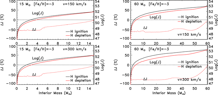
Figure 13. Same as Figure 12 but for models with initial metallicity [Fe/H] = −3.
Download figure:
Standard image High-resolution image4.2. Core He Burning
The evolutionary track of a massive star beyond the central H-burning phase depends on the complex interplay among several factors: (1) the He core that contracts toward a new quasi-equilibrium configuration powered by 3α nuclear reactions, (2) the H-rich mantle that expands toward an RSG configuration, (3) the actual He core mass, and (4) the amount of mass the star loses during this phase. Figure 14 shows the full HR diagram for all our models: the green triangles and red filled dots mark the beginning and end of the central He-burning phase, respectively. Before discussing Figure 14, let us remark that the capability of the mantle of the star to expand (and therefore to become a red giant) on a thermal or nuclear timescale depends on many factors including, e.g., the adoption of the Schwarzschild or the Ledoux criterion in the region of variable H abundance left by the receding H convective core, the opacity of the mantle, and so on. As a consequence, at present, this behavior is still poorly understood.

Figure 14. Evolutionary tracks of all our models on the HR diagram. The various symbols mark the central He-ignition (green triangles), the central He-exhaustion (red dots), and the final position at the presupernova stage (black star).
Download figure:
Standard image High-resolution imageAt [Fe/H] = 0, all of the nonrotating models evolve toward their Hayashi track on a thermal timescale, and therefore they start the core He-burning phase as RSGs, the only exception being the 120  star that loses enough mass to become a WR star already during the core H-burning phase. During this redward excursion, stars with M ≳ 40 M⊙ approach the Eddington luminosity (at log(Teff) ∼ 3.7), lose a substantial fraction of the H-rich envelope, evolve to Blue SuperGiant (BSG) configuration and become WRs (Table 6 shows the time spent by each mass in the various WR subclasses). Less massive stars, on the contrary, reach their Hayashi track and cross the critical temperature for the dust-driven wind to become efficient. However, within this mass interval, only stars with M ≳ 15 M⊙ enter this stage with a central He abundance high enough to have time to lose a consistent amount of mass. When a substantial fraction of the H-rich envelope has been lost, these stars deflate toward a BSG configuration and become WR stars. Stars with M ≲ 15 M⊙ remain RSGs for the entire core He-burning phase. Therefore, at solar metallicity, we predict a population of RSGs up to an initial mass of M ∼ 40 M⊙ (corresponding to a maximum luminosity log(L/L⊙) ∼ 5.7) and a minimum mass for the WR stars of M ∼ 20 M⊙.
At [Fe/H] = −1, nonrotating stars with M ≳ 60 M⊙ quickly expand after the central H exhaustion but never reach their Hayashi track because they lose an enormous amount of mass when they exceed their Eddington luminosity (at log(Teff) ∼ 3.7–3.8) and then become WR stars (see Table 6). Stars in the range ∼30–60 M⊙ ignite and burn He as BSGs without entering the WR phase at all because of the modest mass loss. Stars with M ≲ 30 M⊙ ignite and burn He as RSGs, but none of them crosses the threshold temperature for the condensation of dust, hence they remain RSGs during the entire core He-burning phase. Therefore, at this metallicity, we predict a population of RSGs up to an initial mass of M ∼ 25 M⊙ (corresponding to a maximum luminosity log(L/L⊙) ∼ 5.5) and a minimum mass that enters the WR stage of M ∼ 80 M⊙.
At [Fe/H] = −2 and −3, all nonrotating stars ignite and burn He in the core as BSGs. For these metallicities, therefore, we expect neither RSGs nor WRs during this phase.
Summarizing the results discussed so far, we predict the core He-burning nonrotating models to populate the RSG branch with stars of mass M ≲ 40 M⊙ (log(L/L⊙) ≲ 5.7) at [Fe/H] = 0 and M ≲ 25 M⊙ (log(L/L⊙) ≲ 5.5) at [Fe/H] = −1. No star becomes an RSG at [Fe/H] = −2 and −3. The minimum mass that enters the WR stage during this phase is M ∼ 20 M⊙ at [Fe/H] = 0. No WR star is expected at lower metallicities.
Turning to the evolution of the interior, core He burning occurs, as it is well known, in a convective core that advances progressively in mass until it vanishes at core He depletion. As a consequence, a very steep He profile forms at a mass coordinate corresponding to the maximum extension of the convective core. Such a "typical" behavior fails when mass loss is strong enough to drive the complete ejection of the H-rich mantle and to erode part of the He core. Since the properties of the He-burning phase depend mainly on the actual He core mass, if the He core shrinks while central burning is still active, (1) the He convective core progressively shrinks in mass, leaving a region of variable chemical composition, (2) the surface luminosity progressively decreases, (3) the core He-burning lifetime increases, and (4) the CO core mass at the end of the He-burning phase decreases while the 12C mass fraction increases. Since all of these effects are driven by mass loss, they tend to progressively disappear as the initial metallicity decreases. Figure 15 shows the CO core mass as a function of the initial mass at the core He-exhaustion phase for the four metallicities. As expected, the CO core scales directly with the initial mass at all four metallicities. Similarly to the trend shown by the He core (see Figure 9), the MCO–Mini relation is basically independent of the initial metallicity when mass loss does not erode the He core mass. Therefore, only the solar-metallicity stars of mass M > 40 M⊙ show evident bending due to the decrease of the He core mass.

Figure 15. MCO–MINI relation for the four metallicities. The horizontal dashed line marks the mass limit above which a star enters the pulsation pair instability regime and explodes as a pulsation pair instability supernova.
Download figure:
Standard image High-resolution imageThe inclusion of rotation makes the picture discussed so far even more complex because its effect on the evolution of a star depends on the mass and the metallicity. As in the nonrotating case, at [Fe/H] = 0, we can identify ranges of models that (1) become WR during the core H-burning phase and hence burn He in the core as BSGs, (2) approach their Eddington luminosity during the redward excursion, evolve toward a BSG configuration, and burn He in the core as WR stars, and (3) approach their Hayashi track, enter the dust-driven wind stage, and then turn again to the blue, sometime during the He-burning phase. The basic rule is that the higher the initial rotation velocity, the lower the limiting masses that divide these three mass intervals (Table 5). Note that, for this metallicity, all rotating models end their He-burning lifetime as WR stars since in this case even the two smaller masses are pushed beyond the threshold temperature for dust formation early enough to have time to lose a large part of their mantle and turn again toward the blue (Table 6).
At metallicities [Fe/H] ≤ −1, the quite complex interplay between metallicity and rotation no longer leads to a strictly monotonic trend with the mass. We can identify models that (1) move redward toward the Hayashi track on a thermal timescale, lose a substantial amount of mass because they approach their Eddington luminosity, turn to the blue, and burn He as WR stars (Table 6); (2) ignite He as BSGs, move redward while core He burning goes on, become RSGs, turn to the blue sometime during core He burning, and become WR stars; (3) ignite He as a BSG, move redward on a nuclear timescale, eventually reaching the RSG phase when the central He abundance is more than halved; and (4) ignite and burn He as RSGs. The basic rule in this case is that, on average, the limiting masses that divide the above-mentioned mass intervals decrease by increasing the initial rotation velocity and by decreasing the initial metallicity (Table 5). Note that at these metallicities, no model crosses the temperature threshold (van Loon et al. 2005) to activate the mass loss due to the dust formation.
As in the core H-burning phase, in the core He-burning phase, the interplay among convection, meridional circulation, and shear turbulence also drives the outward transport of angular momentum and mixing of the chemicals.
A quantitative determination of the variation of the angular momentum contained in the He core in this phase depends on the definition of the He core mass. Figure 16 shows the variation of the amount of angular momentum in the He core for the solar-metallicity case and initial velocity 300 km s−1. The two lines correspond to two different choices for the He core mass. If we choose as the He core the amount of mass contained within the H-burning shell, we obtain the red line in the figure. In this case, the progressive advance of the H burning shell continuously adds new mass, and hence angular momentum, to the He core, and this increase is much larger than the amount of angular momentum that flows from the center outward. However, stars more massive than 20  lose a consistent fraction of their He core mass through the wind, and this phenomenon prevails in determining the amount of angular momentum left in the He core. If, conversely, we fix the He core mass just at the beginning of the He-burning phase and compute over the entire He-burning phase the total amount of angular momentum contained within this mass, the scenario changes completely (black line in Figure 16). In this case, the angular momentum always decreases because the mass is fixed and the angular momentum fluxes outward. Note that above 20
  the red and black lines converge, because in both cases, the angular momentum present in the He core is dictated by the mass loss. At subsolar metallicities, the amount of angular momentum that fluxes outward through a fixed He core mass is quite similar to the solar case, so that the decrease of angular momentum varies between 40% and 10% in the range 13 to 25
  . The angular momentum decrease in the more massive stars, similarly to what happens in the solar case, depends on the efficiency of the mass loss. Though rotating massive stars enter the instability region where L/Ledd > 1 and therefore lose a large fraction of their envelope, they do not lose as much mass as their solar counterparts so that the total amount of angular momentum left in the He core at the time of core He depletion also increases moderately as the initial metallicity decreases.
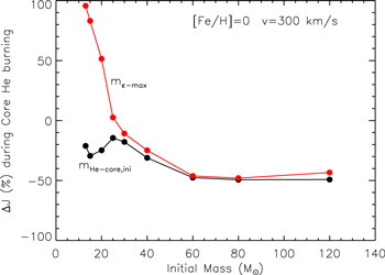
Figure 16. Variation (in per cent) of the total amount of angular momentum stored in the He core, during core He burning, for the solar-metallicity case, computed for two different definitions of the He core mass. The red line refers to the case in which the He core mass is defined at each time at the mass location where maximum nuclear H burning occurs, while the black one refers to the case in which the He core mass is fixed at the beginning of the central He-burning phase and kept constant in time.
Download figure:
Standard image High-resolution imageThe mixing of the chemicals due to rotation-induced instabilities has essentially two basic consequences: (1) the increase of the CO core mass and (2) the exchange of matter between the two active burning regions, i.e., the He convective core and the H-burning shell.
Figure 17 shows the trend of the CO core mass (left y-axis) as a function of the initial mass for the three initial velocities as solid lines. Each of the four panels refers to a specific [Fe/H]. The dotted lines in the same figure show the percentage difference between the nonrotating and rotating models, i.e.,  (right y-axis). The blue lines refer to vini = 150 km s−1 while the red ones to vini = 300 km s−1. The two dotted lines clearly show that, in almost all cases, rotation increases the CO core mass and that the smaller the mass, the larger the increase. Such a trend is basically due to the combination of two effects: (a) the He-burning lifetime scales inversely with the He core mass (and hence, in most cases, the initial mass) so that the smaller the He core mass, the longer the secular instabilities may operate, and (b) the trend with mass is seen in models computed with a constant initial equatorial rotation velocity (see the comment at the beginning of Section 4). The general direct scaling of the CO core with the initial rotation velocity fails when the He core mass is eroded by mass loss. In these cases, in fact, the convective core (and therefore the final CO core mass) shrinks according to the actual He core mass. At [Fe/H] = 0 and [Fe/H] = −1, the most massive rotating stars lose much more mass than their nonrotating counterparts, and this explains why in these cases, the final CO core scales inversely with the initial rotation velocity. At solar metallicity, rotation roughly doubles the CO core mass of the less massive stars but its influence on MCO progressively decreases as the mass increases, becoming almost negligible for stars with M ≥ 40 M⊙. In the more massive models with initial rotation velocity v = 300 km s−1, the global effect of mass loss overcomes the effect of rotation, resulting in a reduction of the CO core mass in rotating models of up to ∼30%–40% for the 120 M⊙ star. At metallicities lower than solar, mass loss decreases dramatically, and therefore its effect on the CO core mass becomes progressively negligible. The spread in the CO core mass–initial mass relations evident in the four panels of Figure 17 (due to the variation of both the initial metallicity and velocity) vanishes if the CO core mass is ranked as a function of the He core mass (Figure 18). The reason is obviously that the evolution of the star after core He depletion is essentially driven by the mass of the He core. Figure 18 shows that CO core masses larger than 35 M⊙ correspond to He core masses larger than 45 M⊙, which is roughly the minimum mass entering the pulsation pair instability regime, as reported by Heger & Woosley (2002). Let us note that this value has also been adopted by Chatzopoulos & Wheeler (2012), Yoon et al. (2012), and Georgy et al. (2017) for their works on pair instability supernovae (PISNe).
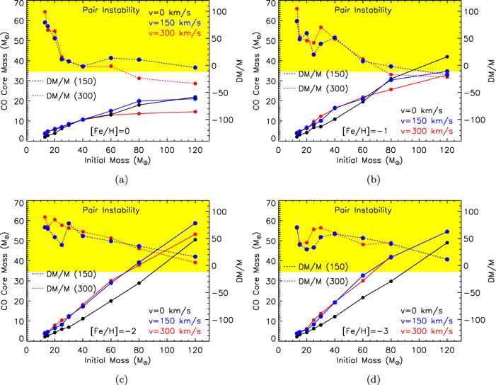
Figure 17. The four panels show, for each initial metallicity, the MCO–MINI relation obtained for the nonrotating (black) and the rotating cases, 150 km s−1 (blue) and 300 km s−1 (red), as solid lines (left Y-axis). The dashed lines show the per cent difference (DM/M) between rotating and nonrotating MCO (right y-axis).
Download figure:
Standard image High-resolution imageAn obvious consequence of the increase of the CO core with rotation is that the minimum mass entering the pulsation pair instability regime decreases as the initial rotation velocity increases (yellow area in Figure 17).
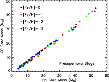
Figure 18. CO core mass as a function of the He core mass for all of the computed models.
Download figure:
Standard image High-resolution imageThe diffusion of chemicals between the He convective core and the H-burning shell, induced by rotation-driven mixing, profoundly changes the chemical composition of the He core. In fact, fresh 12C synthesized in the core He-burning phase diffuses up to the H-burning shell, where it is quickly converted not just into  but also into all the other CNO nuclei, whose relative abundances are dictated by the temperature of the H shell. This means that all of the nuclei involved in the CNO cycle are actually increased by this interplay. The fresh CNO nuclei, and in particular
  , plus fresh He, are brought back toward the center. The
  that diffused back to the center is quickly converted into
  first and then into
  , becoming therefore an efficient primary neutron source. It must not be ignored that the He brought toward the center also plays an important role since it favors the conversion of 12C into 16O, lowering therefore the final 12C/16O ratio in the CO core.
Figure 19 shows the central abundance of 12C at the central He-exhaustion phase for all of the models of our grid as a function of the CO core mass. The effect of rotation-induced mixing on the amount of  left from He burning is readily visible in the large spread of abundances present at the lower CO core masses. The spread reduces progressively as the CO core mass increases because both the timescale over which the instabilities may operate reduces (because the He-burning lifetime scales inversely with the CO core mass) and because we chose a constant initial rotation velocity as a function of mass (see Section 4).
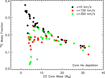
Figure 19. Central 12C abundance at the core He-exhaustion phase for all models of our grid as a function of the core CO mass.
Download figure:
Standard image High-resolution imageAn easy way to quantify the efficiency of the rotation-induced mixing in increasing the initial global abundance of the CNO nuclei is by defining the following quantity (see, e.g., Chieffi et al. 1998):
Such a total abundance (by number) remains constant in nonrotating stars during the central He-burning phase because the  (the most abundant of the CNO nuclei at the central He-ignition phase) left by the H burning may only evolve through the sequence that leads at most to the synthesis of
  , keeping unaltered the total sum (by number) of these nuclei over the entire central He-burning phase.
Conversely, if fresh 14N is brought to the convective core, the χ(N, Mg) parameter necessarily increases. Figure 20 shows the variation of χ(N, Mg) during the core He-burning phase (Δχ(N, Mg)He-burn) for all models with initial rotation velocity v = 300 km s−1 as a function of the initial metallicity. The figure clearly reveals the existence of two different behaviors: (1) in stars with mass M < 40 M⊙, Δχ(N, Mg)He-burn does not show a monotonic dependence on the metallicity, but the maximum variation remains confined within a factor of ∼7 (the only exception being the 13 M⊙ models, left panel in Figure 20), and (2) in stars with mass M ≥ 40 M⊙, on the contrary, Δχ(N, Mg)He-burn scales inversely with the initial metallicity and shows a larger variation of up to a factor of ∼20 (right panel in Figure 20). It is worth noting, however, that the range of metallicity over which the variation of Δχ(N, Mg)He-burn is evaluated, spans three orders of magnitude. The origin of the different behaviors shown in Figure 20 is difficult to understand because the efficiency of rotation-driven mixing depends, in general, on the diffusion coefficients corresponding to the shear instabilities and the meridional circulation (see Equations (2) and (5) in Chieffi & Limongi 2013 and Equation (4.3) in Maeder & Zahn 1998) that, in turn, depend in a very complex way on many interior properties of the He core among which are the local value of the angular velocity and its gradient, the mass and the extension of the He core, the mean molecular weight gradient, the difference between the radiative and the adiabatic gradients, and so on. In addition to these, mass loss may play a crucial role in the primary 14N production. In fact, if mass loss is efficient enough to remove the entire H-rich envelope, it cancels out the engine (i.e., the H-burning shell) needed to convert 12C into 14N. Such an occurrence does not imply that the central value of χ(N, Mg) can no longer increase (because the radiative part of the He core is in any case still very 14N rich), but simply that its increase is reduced with respect to the one that the star would have without the removal of the H shell. Of course, the earlier such a removal occurs, the earlier the conversion of 12C into 14N stops. This phenomenon becomes progressively more important as the mass and metallicity increase because of the direct scaling of the efficiency of mass loss with these two quantities. As we have mentioned above, the primary 14N production may have important consequences on the synthesis of the s-process nuclei at various metallicities—we will address this issue in Section 5.1.

Figure 20. Scaling of Δχ(N, Mg)He-burn (see the text for the definition of this parameter) with the initial metallicity for models of initial rotation velocity v = 300 km s−1.
Download figure:
Standard image High-resolution imageOnce He is exhausted in the center, the CO core starts contracting again while the He burning shifts to a shell where a He convective shell forms. If mass loss did not erode the He core during the central He-burning phase, or if the star did not rotate, the He convective shell forms above the He discontinuity left by the progressive advance of the convective core, in a region with a flat He profile where no products of He burning are present. Conversely, if the mass loss was efficient enough to erode the He core mass while the star was still in the central He-burning phase or if rotation-induced mixing modified the chemical composition of the intershell, the He convective shell forms in a region that has a pronounced He profile either left over by the receding He convective core (if the He core is reduced by mass loss) or determined by the continuous exchange of matter between the convective core and the H shell burning (in rotating models).
4.3. Advanced Nuclear-burning Stages
In the previous section, we showed that all models that develop a CO core more massive than ∼35 M⊙ at core He-depletion enter the pulsation pair instability regime. This occurs when the adiabatic index Γ1 drops below ∼4/3 in a substantial fraction of the core, which therefore becomes unstable. This instability is usually encountered during core O burning, but it may also occur either in core C burning or core Si burning, depending on the physical conditions of the interior of the star. Once the instability sets in, we stop the calculations; in the following, we will describe the evolutionary properties of all the models that do not enter the pulsation pair instability regime.
Rotation (at least in the range of initial rotation velocities considered in this paper) does not significantly affect the evolutionary properties of a star beyond the He-burning phase because (1) the timescales over which the rotation instabilities operate are much longer than the advanced evolutionary timescales, so that they do not have enough time to operate, and (2) the local gravity in the core dominates over the centrifugal force, preserving therefore a quasi-spherical shape (see CL13). Also, the initial metallicity does not play any direct role in the physical evolution of a star in the advanced burning phases because all of the relevant nuclear reactions involve primary nuclei. In other words, the evolution of a star in the advanced burning phases is no longer linked to its initial mass, metallicity, and initial rotation velocity, but it is controlled essentially by the mass of the CO core (which in all respects plays the role of the "total" mass) and the amount of 12C left after core He burning (the main fuel that powers both the C and the Ne burning). The role of the initial metallicity and rotation velocity influences the advanced burning only through their capability to modify the mass of the CO core as well as the abundance of 12C at the end of the core He-burning phase.
As already discussed in the previous section, there is a quite tight correlation between MCO and the 12C left after core He burning for MCO ≥ 15 M⊙ or so, the reasons being either the fact that in any case the 12C/16O ratio scales inversely with the size of the He core mass or that the choice of an initial rotation velocity independent of the mass implies a progressive reduction of the effects induced by rotation as the initial mass increases. For these core masses, therefore, the only parameter that controls the advanced burning phases is the CO core mass. Stars that develop MCO ≤ 15 M⊙, conversely, cannot be ranked just in terms of the mass of the CO core; they constitute a family of models, each of which depends on two parameters that are not much correlated.
Since the compactness of a star at the beginning of the collapse scales directly with the CO core mass and inversely with the 12C abundance left after He burning, and since both Figures 18 and 19 show that in most cases the CO core mass scales inversely with the initial metallicity and directly with the initial rotation velocity, we can conclude that a reduction of the initial metallicity and/or an increase of the initial rotation velocity produces, in general, more compact cores.
The compactness of a star at the presupernova stage is a fundamental property that influences the dynamics of the core collapse and the following explosion. In the past, we usually discussed the compactness of a star in terms of the mass–radius relation (or density profile) at the presupernova stage. In recent years, it has become very popular to use a single or a few parameters to describe such a property. For example, O'Connor & Ott (2011) define the compactness by means of the parameter  , while Ertl et al. (2016) defined it by means of the two parameters M4 and μ4 (their Equations (2) and (3)). Just as an example, we show in Figure 21 how the ξ2.5 parameter, evaluated at the presupernova stage, scales with the CO core mass. It is interesting to note that Figure 21 shows a rather tight relation between the ξ2.5 and the CO core mass. Such a tight relation becomes much more scattered if the ξ2.5 parameter is ranked as a function of the initial mass (Figure 22).

Figure 21. Plot of the compactness parameter  as a function of MCO for all models, rotating or not.
Download figure:
Standard image High-resolution image
Figure 22. Same as Figure 21 but now as a function of the initial mass.
Download figure:
Standard image High-resolution imageWhile the dramatic shortening of the lifetimes of the advanced evolutionary stages, determined by the enormous neutrino energy losses due to pair production, largely inhibits any transport of the angular momentum in the radiative zones, in the convective regions, we assume that angular momentum transport is so efficient that we impose a flat profile of the angular velocity. Note that, in all models of the present grid, no convective region crosses the outer edge of the CO core; therefore, the total angular momentum stored in the CO core will remain constant up to the onset of the iron core collapse.
The surface properties (luminosity, radius, and chemical composition) of a massive star at the time of the explosion is an important theoretical prediction since they are an "observable," in the sense that they control the way in which the supernova will appear to the observer (as a Type II, IIb, Ib etc.). The black stars in Figure 14 mark the positions of the models at the presupernova stage in the HR diagram. Note that in some cases, stars move, even substantially, from their position at the core He-exhaustion phase (red dots). Table 7 summarizes the main properties of all presupernova models of the present grid. The various columns refer to the initial mass (column 1); the amount of H in the envelope (column 2); the amount of He in the envelope (column 3); the mass of the iron core (column 4), defined as the mass coordinate corresponding to the sharp drop of the electron profile below ∼0.49; the binding energy of the mass above the iron core (column 5); the compactness parameter ξ2.5 (column 6); the angular momenta contained within the iron core (column 7), the CO core (column 8), the He core (column 9), the inner 1.5 M⊙ (column 10), and the inner 2.0 M⊙ (column 11); and the expected SN type, according to the classification suggested by Hachinger et al. (2012).
Table 7. Properties of the Presupernova Models
| Initial Mass | H | He | MFe | Ebind | ξ2.5 | JFe | JCO | JHe | J1.5 | J2.0 | SN Type |
|---|---|---|---|---|---|---|---|---|---|---|---|
| (M⊙) | (M⊙) | (M⊙) | (M⊙) | (1051 erg) | (1051 erg s) | (1051 erg s) | (1051 erg s) | (1051 erg s) | (1051 erg s) | ||
| [Fe/H] = 0 v = 0 km s−1 | |||||||||||
| 13 | 5.37 | 4.31 | 1.36 | 0.65 | 0.02 | 0.000 | 0.000 | 0.000 | 0.000 | 0.000 | SNIIP |
| 15 | 5.67 | 4.63 | 1.43 | 0.95 | 0.12 | 0.000 | 0.000 | 0.000 | 0.000 | 0.000 | SNIIP |
| 20 | 0.06 | 3.39 | 1.10 | 2.00 | 0.14 | 0.000 | 0.000 | 0.000 | 0.000 | 0.000 | SNIb |
| 25 | 0.00 | 2.26 | 1.38 | 2.24 | 0.15 | 0.000 | 0.000 | 0.000 | 0.000 | 0.000 | SNIb |
| 30 | 0.00 | 2.74 | 1.57 | 4.75 | 0.38 | 0.000 | 0.000 | 0.000 | 0.000 | 0.000 | SNIb |
| 40 | 0.00 | 2.49 | 1.53 | 6.17 | 0.37 | 0.000 | 0.000 | 0.000 | 0.000 | 0.000 | SNIb |
| 60 | 0.00 | 0.93 | 1.52 | 9.28 | 0.44 | 0.000 | 0.000 | 0.000 | 0.000 | 0.000 | SNIb |
| 80 | 0.00 | 1.10 | 1.66 | 15.80 | 0.48 | 0.000 | 0.000 | 0.000 | 0.000 | 0.000 | SNIb |
| 120 | 0.00 | 1.05 | 1.91 | 22.61 | 0.51 | 0.000 | 0.000 | 0.000 | 0.000 | 0.000 | SNIb |
Only a portion of this table is shown here to demonstrate its form and content. A machine-readable version of the full table is available.
Download table as: DataTypeset image
On the basis of all the results discussed so far ,we predict that at solar metallicity and vini = 0, stars less massive than 20  explode as RSGs while the more massive ones explode as WR stars. The relative numbers among the WNL, WNE, WNC, and WC obviously depend on the total amount of mass lost: the present set of models predicts a much larger number of WNE and WC with respect to the WNL, and no WNC. According to the supernova classification of Hachinger et al. (2012), we predict that the maximum mass exploding as SNIIP ranges between 15 < MIIP < 20 M⊙, while stars more massive than MIb ∼ 20 M⊙ explode as SNIb. We cannot determine (for any initial metallicity) the range of masses that explode as Type IIb because they are intermediate between SNIIP and the SNIb, and our grid is not refined enough to allow us to determine their mass interval. At [Fe/H] = −1, mass loss decreases, and hence the maximum mass that explodes as an RSG increases up to a mass in the range 60 < MIIP < 80 M⊙, with the more massive stars reaching collapse as either WNL or WC, and exploding as an pulsation pair instability supernova SNIb. At this metallicity, the minimum mass that becomes a pulsation pair instability supernova (PPISN) ranges between 100 < MPPISN < 120 M⊙. At [Fe/H] ≤ −2, mass loss decreases so much that no star loses a large fraction of its H-rich mantle, and hence no star becomes a WR. Stars less massive than ∼25–30 M⊙ explode as RSGs while stars above this limiting value explode as BSGs. At these low metallicities, all stars explode as SNIIP. The minimum mass exploding as a PPISN ranges now between 60 and 80
  .
.
Rotation favors the redward evolution at the end of the central H-burning phase, and in many cases, it also pushes stars above the Eddington luminosity, strongly enhancing mass loss. Hence, on one hand, it increases the maximum mass that explodes as an RSG but it also lowers the minimum mass that enters the WR stage, squeezing therefore the range of masses that reach the core collapse as a BSG. Note, however, that the interplay between rotation and mass loss has a complex and nonmonotonic impact on the expected number of the various types of WR supernovae and that, in any case, at variance with the nonrotating case, it allows some progenitors to explode as WNC stars. As a general trend, at any given initial metallicity, both MIIP and MIb decrease as the initial rotation velocity increases. Also, the minimum mass that explodes as a PPISN decreases as the rotation velocity increases because of the direct scaling of the CO core mass with the rotation velocity (see above).
5. The Yields
The chemical composition of the ejecta of each stellar model after the explosion has been computed as described in CL13. Since this approach is not based on first principles, a proper calibration of the explosion is necessary. Such a calibration is obtained by requiring a fit to some observable, typically the amount of  ejected and/or the final kinetic energy of the ejecta. The choice of the calibration is crucial because it directly affects the location of the mass cut and hence the yields of many nuclei (basically those produced by the explosive burning). In our previous set of models (CL13), the yields were computed by assuming that all stars eject 0.1
  of
of  . In this paper, conversely, we computed three different sets of yields obtained for different choices of the mass cut in order to show which is the consequence of each choice (other calibrations may be provided upon request). The first set of yields (set F) is obtained as in our previous paper, i.e., assuming that the stars eject a fixed amount of
  (0.07
(0.07  in this case). The second one (set M) is obtained by adopting the mixing and fallback (MFB hereinafter) scheme (Umeda & Nomoto 2002): for each star, the inner border of the mixed region is fixed by requiring that [Ni/Fe] = 0.2 and the outer one is fixed at the base of the O-burning shell; the mass cut is then chosen by assuming once again that each star ejects 0.07
  of
of  . The third set (set R), which is our recommended one, is obtained by assuming that all stars in the range 13–25
  behave like those in set M, while those more massive than 25
  fully collapse to a black hole, and therefore their yields include only the stellar wind. The yields of all the models of set R are reported in Table 8. Since, as already mentioned above, for the set R the yields of stars with M > 25 M⊙ are those present in the wind, for the sake of completeness we report in Table 9 the yields present in the wind of all the stars with mass M ≤ 25 M⊙. Note that also the yields of the stellar models that we predict to explode as PPISNe refer only to the wind because we could not follow their evolution once they enter the pair instability regime (see above).
Table 8. Isotopic Yields—Recommended Set
| Isotope | 13 M⊙ | 15 M⊙ | 20 M⊙ | 25 M⊙ | 30 M⊙ | 40 M⊙ | 60 M⊙ | 80 M⊙ | 120 M⊙ |
|---|---|---|---|---|---|---|---|---|---|
| v = 0 km s−1; [Fe/H] = 0 | |||||||||
| H | 6.1592E+00 | 6.8845E+00 | 8.5593E+00 | 1.0135E+01 | 1.1576E+01 | 1.4539E+01 | 2.0463E+01 | 2.5220E+01 | 3.6732E+01 |
| H2 | 2.9523E−06 | 3.6682E−06 | 5.8878E−06 | 7.3598E−06 | 8.8318E−06 | 1.1777E−05 | 1.7670E−05 | 2.3570E−05 | 3.5377E−05 |
| H3 | 5.4069E−29 | 3.1300E−26 | 2.0669E−16 | 4.3294E−14 | 2.2082E−13 | 2.6141E−12 | 1.4364E−11 | 4.3895E−11 | 1.3806E−10 |
| He3 | 3.6548E−04 | 3.9439E−04 | 4.6986E−04 | 5.4836E−04 | 6.2781E−04 | 7.8911E−04 | 1.1168E−03 | 1.3396E−03 | 1.7584E−03 |
| He4 | 4.6327E+00 | 5.1226E+00 | 7.1652E+00 | 8.3288E+00 | 7.3349E+00 | 1.0974E+01 | 2.1610E+01 | 3.0098E+01 | 5.1977E+01 |
| Li6 | 5.9770E−11 | 7.4266E−11 | 1.1972E−10 | 1.5018E−10 | 1.8090E−10 | 2.4319E−10 | 3.6984E−10 | 4.9849E−10 | 7.5772E−10 |
| Li7 | 8.4900E−10 | 1.0549E−09 | 1.7985E−09 | 2.2774E−09 | 2.7630E−09 | 3.8796E−09 | 5.6519E−09 | 7.2343E−09 | 1.1083E−08 |
| Be7 | 1.4797E−18 | 4.6861E−16 | 1.1940E−14 | 4.7919E−12 | 8.4431E−12 | 1.1629E−11 | 2.0945E−11 | 1.5975E−11 | 3.0266E−12 |
| Be9 | 2.2919E−11 | 2.6008E−11 | 6.2224E−11 | 7.6757E−11 | 9.1030E−11 | 1.1843E−10 | 1.7102E−10 | 1.9062E−10 | 2.9079E−10 |
| Be10 | 1.0346E−59 | 1.1587E−59 | 5.8796E−60 | 6.5850E−60 | 0.0000E+00 | 0.0000E+00 | 0.0000E+00 | 0.0000E+00 | 0.0000E+00 |
| B10 | 2.5435E−10 | 2.8155E−10 | 3.8508E−10 | 5.9700E−10 | 6.9818E−10 | 8.9221E−10 | 1.2645E−09 | 1.4327E−09 | 2.1285E−09 |
| B11 | 8.0392E−09 | 8.9875E−09 | 1.1279E−08 | 1.3480E−08 | 1.5659E−08 | 2.0470E−08 | 3.0119E−08 | 3.7374E−08 | 5.4080E−08 |
| C12 | 1.1404E−01 | 2.2096E−01 | 4.0941E−01 | 6.1944E−01 | 2.5054E−02 | 3.1933E−02 | 3.9826E−01 | 1.1226E+00 | 2.0178E+00 |
| C13 | 6.9180E−04 | 7.7869E−04 | 1.0411E−03 | 1.2839E−03 | 1.4423E−03 | 1.8031E−03 | 1.7254E−03 | 1.7021E−03 | 2.3899E−03 |
Only a portion of this table is shown here to demonstrate its form and content. A machine-readable version of the full table is available.
Download table as: DataTypeset image
Table 9. Isotopic Yields in the Wind—Recommended Set
| Isotope | 13 M⊙ | 15 M⊙ | 20 M⊙ | 25 M⊙ |
|---|---|---|---|---|
| v = 0 km s−1; [Fe/H] = 0 | ||||
| H | 7.9437E−01 | 1.2188E+00 | 8.5000E+00 | 1.0135E+01 |
| H2 | 2.9523E−06 | 3.6682E−06 | 5.8878E−06 | 7.3598E−06 |
| H3 | 1.7054E−30 | 3.1250E−26 | 2.0669E−16 | 4.3294E−14 |
| He3 | 4.6963E−05 | 6.9968E−05 | 4.6986E−04 | 5.4836E−04 |
| He4 | 3.1961E−01 | 4.9952E−01 | 3.7908E+00 | 6.1010E+00 |
| Li6 | 5.9770E−11 | 7.4266E−11 | 1.1972E−10 | 1.5018E−10 |
| Li7 | 8.4900E−10 | 1.0549E−09 | 1.7985E−09 | 2.2774E−09 |
| Be7 | 8.1083E−25 | 1.1721E−23 | 7.2389E−17 | 4.7919E−12 |
| Be9 | 1.6797E−11 | 2.0871E−11 | 6.2224E−11 | 7.6757E−11 |
| Be10 | 0.0000E+00 | 0.0000E+00 | 0.0000E+00 | 0.0000E+00 |
| B10 | 9.5849E−11 | 1.2419E−10 | 3.8508E−10 | 5.9700E−10 |
| B11 | 1.2602E−09 | 1.8599E−09 | 1.1279E−08 | 1.3480E−08 |
| C12 | 1.7190E−03 | 2.6176E−03 | 1.7858E−02 | 2.1608E−02 |
| C13 | 8.2730E−05 | 1.2971E−04 | 1.0112E−03 | 1.2679E−03 |
Only a portion of this table is shown here to demonstrate its form and content. A machine-readable version of the full table is available.
Download table as: DataTypeset image
Let us start the analysis of the yields by showing the relative contributions of the stars in the ranges 13 ≤ M/M⊙ ≤ 25 (LINT) and 25 < M/M⊙ ≤ 120 (UINT) to the total yields integrated over a standard Salpeter initial mass function (IMF) having the slope x = 1.35. Figure 23 shows, for set M, the relative contributions of the LINT (solid bars) and UINT (hatched bars) groups to the yield of each element. The color coding identifies the elements that are under-, co-, and overproduced with respect to O: those moderately underproduced with respect to O (−0.6 ≤ [X/O] < −0.3) are marked green, the ones more or less coproduced with O (−0.3 ≤ [X/O] ≤ 0.3) are in blue, while those overproduced with respect to O ([X/O] > 0.3) are red. The elements that do not have any bar are those severely underproduced with respect to O and therefore are the ones for which it is irrelevant to determine which mass interval contributes most to their yields. O is adopted as the leading element because it is either the most abundant element after H and He, and it is also almost exclusively produced by massive stars.
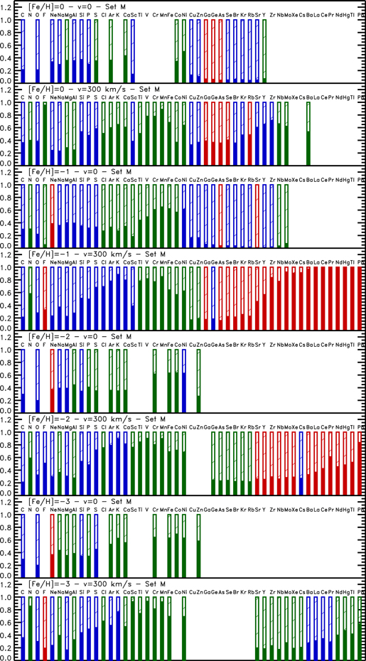
Figure 23. Relative contributions of the stars in the ranges 13 ≤ M/M⊙ ≤ 25 (solid bars) and 25 < M/M⊙ ≤ 120 (dashed bars) to the total yields integrated over a standard Salpeter IMF (x = 1.35). The elements underproduced with respect to oxygen by a factor between 0.25 and 0.5 are marked green, those coproduced (i.e., in the interval 0.5 and 2) are blue, while those overproduced (i.e., by more than a factor of 2) are red. The missing bars mean that the corresponding elements are largely underproduced (less then 0.25) with respect to O.
Download figure:
Standard image High-resolution imageWe remind the readers that if we define PFX as the production factor of a given element "X" averaged over a Salpeter IMF between 13 and 120 M⊙, the [X/O] ratios are simply the log10(PFX) vertically shifted by log10(PFO) (with a minor correction due to the enhancement of the alpha elements), and hence that the [X/O] basically share the same properties as the PFs: in particular, they directly show which elements are produced by massive stars and which do not (clearly all of the elements that have [X/O] close to zero are coproduced with O and hence are produced mainly by massive stars). Obviously, a flat distribution of the PFs produced by a generation of stars would imply that their ejecta preserve the relative scaling of the initial composition.
In the absence of rotation (first, third, fifth and seventh panels in Figure 23), the LINT group contributes to the synthesis of the elements C to Ni between ∼20%–50% in most cases. Elements between the Fe peak and the first neutron closure shell are produced preferentially by the UINT group down to [Fe/H] = −1, while they are basically not produced by massive stars at lower metallicities. No element beyond the first neutron closure shell is produced by nonrotating massive stars.
Figure 24 shows a comparison of the [X/O] obtained in the three sets, F (red)–M (green)–R (blue), for the nonrotating, solar-metallicity models. This figure shows that in a scenario in which all of the stars eject 0.07  of
of  (set F, red dots), the intermediate-mass elements, i.e., elements from O to Ca, are basically coproduced with O and hence produced by massive stars. F, Mg, Cl, and K are the only ones significantly underproduced with respect to O but, while F is probably produced by intermediate-mass stars, Mg, Cl, and K could in principle constitute a problem because no other source for their production has been identified so far. The block of Fe-peak nuclei (Sc–Zn) is significantly (and correctly) underproduced with respect to O, since these elements are mainly produced by SNe Ia. The elements Ga to Zr, the so-called s-weak component, are more or less coproduced with O, the only exceptions being Ga and As that are slightly overproduced; this result confirms the general belief that massive stars contribute significantly to the synthesis of these elements. The [X/O] of all elements heavier than Zr drops quickly well below zero, which means that they are not produced by massive stars.

Figure 24. Comparison among the [X/O] obtained for the three different sets of yields, F (red), M (green), and R (blue), of nonrotating, solar-metallicity stars. See the text for a definition of the three sets.
Download figure:
Standard image High-resolution imageA comparison between sets F (red) and M (green) in Figure 24 shows the effect of the MFB, at least in the framework of the parameters (inner and outer borders of the mixed zone and final mass cut) described above. The differences between the two sets are obviously confined to the elements mainly produced in the more internal zones by explosive burning. In particular, the [X/O] of Si ( ), S (
 ), Ar (
 ), Ca (
 ), Ti (
 ), V (
 ), Cr (
 ), and Mn (
 ) decrease in set M. By the way, we report in the parentheses either the most abundant isotope of that element if it is synthesized directly, or its parent isotope if it is fed from the decay of another isotope. The reason for such a decrease is that these elements are mostly synthesized by incomplete explosive Si burning and/or explosive O burning, in regions more external than those where
  is produced. Therefore, the MFB mechanism spreads them back to a region that remains locked in the remnant. Ni, on the contrary, shows the opposite behavior, its [X/O] slightly increasing in set M. The reason is that Ni (
 ) is basically produced by complete explosive Si burning, in zones more internal than those where
  is synthesized, and in this case, the effect of the MFB is to mix some
  from the region where it would be locked in the remnant into the one that is then ejected, therefore raising its yield. It is worth noting that the odd–even effect, usually interpreted in terms of initial metallicity, is actually significantly affected by the possible presence of MFB. In fact, while the yields of the α elements Si, S, Ar, and Ca are lowered by the MFB (see above), the ones of P, Cl (
 ), and K (
 ) remain basically constant because they are mainly synthesized (at solar metallicity) in the C convective shell, which is not affected by the MFB. For the sake of completeness, we remind readers that the other, much less abundant, isotopes of Cl and K, namely
  ,
,  , and
, and  , are mainly produced by He burning. Sc and Co deserve specific comments because they are usually considered elements produced by explosive burning (and hence they should be affected by the MFB) while, on the contrary, both elements have an important (secondary) contribution from the hydrostatic burning. Sc is produced either as
  by explosive O burning, and as
  and
and  in the shell C burning (plus a minor contribution from the He shell) via neutron captures. Also, Co has a double production site, being synthesized either as
  by complete explosive Si burning and directly as
  by hydrostatic He and C burning (again via n captures). At solar metallicity, the presence of a strong neutron flux favors the hydrostatic production (in the C and He shells) of both of these nuclei with respect to the explosive one. Since the C- and He-burning shells are not affected by the MFB, this explains why these elements are not significantly affected by the presence, or absence, of the MFB. A comparison between set M (green) and R (blue) shows the influence of stars more massive than 25
  on the distribution of [X/O]. The most evident effect of the choice that all stars more massive than 25
  fully collapse to a remnant contributing to the yields only through the wind (set R) is that the overproduction of some elements of the weak component disappears. The reason is clearly due to the fact that these nuclei, which are mainly produced in the C convective shell of the more massive stars, remain locked in the remnant in this case. Conversely, most of the intermediate-mass elements have [X/O] systematically higher (and closer to 0) than those of set "M" because the more massive stars contribute more to the yield of O than to the yields of the intermediate-mass nuclei.
Figure 25 is analogous to Figure 24 but for [Fe/H] = −3. As expected, set F (red) shows a quite flat distribution of the even nuclei between C and Ca because of their primary origin and a consistent odd–even effect due to the low metallicity; elements beyond the Fe peak are not produced at all because of the negligible neutron flux present at this low metallicity (Prantzos et al. 1990; Raiteri et al. 1992, 1993; Chieffi & Limongi 2004). The effect of the MFB (set M, green color) on the [X/O] is qualitatively similar to that seen at solar metallicity. In this case, however, we also find a substantial increase of the abundances of Co, Ni ( ), Cu (
 ), and Zn (
 ). The reason is that these nuclei have a composite production, both explosive and hydrostatic. The hydrostatic component is mainly due to core He burning, while the explosive one is due to complete explosive Si burning (as already discussed above in the case of Co). As the initial metallicity decreases, the hydrostatic component, basically of secondary origin, progressively vanishes, leaving therefore full visibility of the explosive one, which is mainly of primary origin. The effect of the MFB on these elements is therefore similar to the one already discussed for Ni at [Fe/H] = 0. The lack of contribution from the more massive stars (set R, blue) systematically increases, also at subsolar metallicity, the [X/O] of all elements with respect to those of set M because the scaling of the yield of O with the mass is steeper than that of most of the other elements.
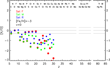
Figure 25. Same as Figure 24 but for [Fe/H] = −3.
Download figure:
Standard image High-resolution imageRotation changes the scenario depicted above. The first thing worth noting is that the contribution of the LINT group to the total yield of most elements increases in rotating models at any metallicity. This is clearly visible in Figure 23 by comparing the four pairs of panels. This result is the consequence of the fact that we chose to adopt the same initial rotation velocity for all of the masses of each given generation of stars. In fact, as has already been mentioned above, since the effects of rotation scale directly with v/vcrit and this parameter scales inversely with the initial mass (Figure 4), the effects of rotation scale inversely with the initial mass. If we now consider that rotating models (on average) have larger yields than their nonrotating counterparts (both because they develop larger He core masses and because of the formation of a primary neutron source), it turns out that the LINT group is more affected by rotation than the UINT group and therefore it tends to prevail in rotating models.
Keeping this in mind, Figure 26 shows in the upper panel a comparison between the [X/O] obtained for nonrotating (red dots) and rotating (300 km s−1, green dots) models, for set M and solar metallicity. In this case, most of the [X/O] show a very modest dependence on the rotation velocity, with the exception of F and the weak component, which are enhanced because of the presence of a primary source of neutrons. It is worth noting that Ne, Na, Mg, and Al tend to have systematically smaller [X/O] in rotating models because their yields depend on the amount of C left from He burning that, in turn, scales inversely with the rotation velocity (see Figure 19 and the discussion above). The lower panel in Figure 26 shows the same comparison but for set R. It is quite evident that now the differences between the rotating and nonrotating models are larger, but are concerned basically with the weak component plus the group formed by Ne, Na, Mg, and Al. The reason is simply that the UINT group contributes more to the yields in the nonrotating models than to those in the rotating ones, so that their substantial removal in set R has a major effect in the nonrotating models while is quite marginal in the rotating ones.

Figure 26. Upper panel: comparison between the [X/O] obtained for nonrotating (red dots) and rotating (300 km s−1, green dots) models, for set M and solar metallicity; the lower panel is the same as the upper panel, but for set R.
Download figure:
Standard image High-resolution imageFigure 27 shows the same comparisons in Figure 26 but for [Fe/H] = −1. The striking difference between the solar and the subsolar metallicity is the high production of F and heavy nuclei up to Pb in the rotating models. This result is due to the large increase of the neutron/seed ratio (i.e., the ratio between the number densities of neutrons and Fe nuclei) in the rotating models as the initial metallicity decreases. In fact, while the primary neutron source—produced by the conversion of fresh  into
into  first and
  later—increases or remains roughly constant as the initial metallicity reduces (this is clearly visible in Figure 20, which shows the trend with metallicity of the primary
  for models rotating at 300 km s−1), the global abundance of the seed nuclei (basically Fe) obviously scales directly with the initial metallicity. This large increase of the neutron/seed ratio as the initial metallicity decreases favors a substantial flux of matter through the bottlenecks corresponding to the two neutron magic numbers N = 50 and N = 82 and hence a consistent flux of matter up to Pb. The capability of a large neutron/seed ratio to push matter up to Pb has been shown by Clayton (1968, Figures 7–22) and has been studied for the first time by Gallino et al. (1998) in low-metallicity, low-mass AGB stars. Both panels in Figure 27 show a high production of heavier nuclei, with set R providing again a larger overproduction because of the dominant contribution of the LINT interval to the yields of the various elements (see the fourth panel in Figure 23). A reduction of the initial metallicity below [Fe/H] = −1 does not lead to a further increase of the [X/O] of the heavier nuclei but actually to their progressive reduction. Figures 28 and 29 show in fact that the very high [X/O] of the elements beyond Zn obtained at [Fe/H] = −1 decrease progressively as the metallicity drops. There are two causes that contribute to such a trend. The first one is that the increase of the abundances of the heaviest nuclei is obtained at the expense of the global abundance of the Fe-peak nuclei, which therefore constitutes the maximum buffer that can be used to build up the heavier nuclei (independently of the neutron flux). In other words, the lower the metallicity, the lower the total amount of matter that can be used to build up the heaviest nuclei. The second reason is that O mildly increases as the metallicity decreases, and therefore this helps in pull down the [X/O] ratios.
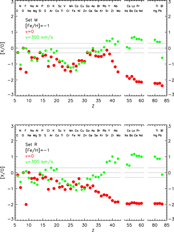
Figure 27. Same as Figure 26, but for [Fe/H] = −1.
Download figure:
Standard image High-resolution image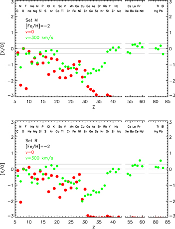
Figure 28. Same as Figure 26, but for [Fe/H] = −2.
Download figure:
Standard image High-resolution image
Figure 29. Same as Figure 26, but for [Fe/H] = −3.
Download figure:
Standard image High-resolution image5.1. N, F, and s-processes
In the previous section, we showed that the formation of a conspicuous primary neutron flux within the He core leads to the synthesis of large amounts of elements like N, F, and heavy nuclei (i.e., those beyond Zn) at subsolar metallicities. It is therefore important to provide additional details about the synthesis of these nuclei in the presence of rotation. Let us repeat here that the diffusion of matter between the H- and He-burning zones largely increases the abundances of all CNO nuclei in the He core. Though the most abundant isotope is obviously  , also
  ,
,  and
and  increase greatly. Part of these nuclei flow in the convective core, but part of them remains locked in the radiative region of the He core. Figure 30 shows, in the upper panel, a typical distribution of the CNO nuclei in the He core of a 20 M⊙ star with [Fe/H] = −1, initially rotating at 300 km s−1: the dashed lines refer to 4He (black),
  (red), and
  (green) (right y-axis), while the solid lines refer to all the other nuclei (left y-axis). The figure shows clearly that the radiative part of the He core is largely enhanced in all CNO nuclei.

Figure 30. Distribution of the CNO nuclei plus those involved in the synthesis of  in the He core of a 20 M⊙, [Fe/H] = −1, and vini = 300 km s−1 star. The dashed lines show the abundances in mass fraction of 4He (black),
  (red), and
  (green) (right y-axis), while the solid lines show the logarithmic abundances (by number fraction) of all the other nuclei (left y-axis). The upper panel shows the internal run of these nuclei at the central He-exhaustion phase, while the lower panel shows the same profiles once the He convective shell has fully developed.
Download figure:
Standard image High-resolution imageThis is an ideal environment for the synthesis of  . To understand why, let us start by recalling that the sequence of reactions that leads to the production of 19F is
  (α, γ)
 (β+)
(β+) (p, α)
 (α, γ)
 (Goriely et al. 1990). The activation of this chain requires a hot environment rich in
  , α particles, and protons. While both 14N and α particles are simultaneously present in the He core, the abundance of protons is negligible, and the most efficient way to produce them in these conditions is through the
  (n, p)
 reaction, which, of course, requires a neutron flux.
  (α, n)
 must be excluded because, at the temperatures at which this nuclear reaction occurs,
  ,
,  and
and  , are already fully converted into
  .
.  (α, n)
 activates at much lower temperatures and is therefore suitable as a neutron source provided that
  is still abundant. The natural place where all these requirements meet together is the He convective shell. In fact, when the He convective shell forms, it engulfs both
  and
and  (present in the outer part of the He core) so that they burn simultaneously:
  captures α particles and emits neutrons, while
  captures either α particles and the just-produced neutrons, synthesizing therefore both the
  and the protons whose further reaction eventually provides the
  necessary to synthesize
  . This sequence of events obviously occurs also in nonrotating models, but in this case the available amount of CNO nuclei is too small to raise significantly the
  abundance. Conversely, in the presence of rotation, there is a large abundance of CNO nuclei in the region where the He convective shell develops (upper panel in Figure 30). The lower panel of Figure 30 shows the profiles of the same isotopes reported in the upper panel, after the He convective shell is fully developed. Note that the region between 6.1 and 8.3
  , i.e., the one in which the He convective shell develops, is the one in which the peaks of
  and
and  are present. The ingestion of both these nuclei leads to a convective shell that eventually becomes greatly enriched in 19F,
  ,
,  , and
, and  , while
  and and
  are partially and fully destroyed, respectively. There are a few additional things worth noting in Figure 30: (a) rotational mixing already increases the number fraction of
  at a level of a few times 10−7 in the He-rich zone (upper panel of Figure 30); therefore, even without a neutron source, it would be possible to raise substantially the 19F abundance; (b)
  is also very abundant and contributes to the neutron flux via the
  (α,n)
(α,n) reaction; (c) at the onset of core collapse, the He convective shell is still largely enriched in
  , which means that additional production of 19F would have been possible if the He shell were not frozen by the very fast evolution of the stellar core in the advanced burning phases. Of course, this complex interplay among the various physical phenomena contributing to the synthesis of 19F implies that we do not expect a strict monotonic dependence of the
  yield on the mass, metallicity, and rotational velocity, but we certainly do expect a large primary production of both
  and
and  in rotating models.
While the synthesis of  is controlled by
  (α, n)
 and occurs in the He convective shell, the large abundances of the elements beyond Zn at subsolar metallicity are due to the activation of
  (α, n)
 during the core He-, radiative shell He-, and convective shell C-burning phases. Figure 31 shows in the upper panel (again for a 20
  star of [Fe/H] = −1 and vini = 300 km s−1) the profiles of a subset of key nuclei at the central He-exhaustion phase (dashed lines), at the formation of the He convective shell (dotted lines), and at the presupernova stage (solid lines). These isotopes have been chosen because they mark the passage of matter through the neutron closure shells at n = 50 (Kr, Rb, Sr, Y, and Zr) and at n = 82 (Ba), and therefore its capability to reach the end point (Pb) of the neutron capture nucleosynthesis. The abundances of these nuclei in the He convective shell at the presupernova stage (between ∼6.1 and ∼8.3 M⊙) are not the result of a He convective shell itself, but mainly the result of the mixing of matter previously synthesized either by the radiative He shell and/or the He convective core. This is clearly shown by a comparison between the dotted and the solid lines (note that the y-scale is logarithmic). Another thing worth noting in the same panel is the contribution of the C convective shell (extending between ∼2.8 and ∼4.2 M⊙). It is clear that there are isotopes that are destroyed, untouched, or produced by the C convective shell. This result is, however, highly misleading if one forgets that explosive nucleosynthesis may alter, even significantly, the chemical composition within the CO core. The lower panel in Figure 31 shows the same nuclei reported in the upper panel, before (dashed line) and after (solid line) the explosion (the minimum value of the x-axis corresponds now to the mass of the remnant). The first thing worth noting is that explosive nucleosynthesis significantly alters the abundances of all the nuclei plotted in the figure, within a substantial fraction of the CO core. In particular,
  ,
,  ,
,  ,
,  , and
, and  are destroyed while
  is produced;
  , on the contrary, is only mildly affected. Of course, each nuclear species will have its own behavior and also the amount of reprocessing will depend on the energy of the explosion. It is not the purpose of this paper to discuss each isotope in detail, but what is important to keep in mind is that, at variance with what is largely accepted, explosive burning cannot be ignored when computing the yields of almost all of the nuclear species. In this case, for example, only the zones more external to ∼5.3 M⊙, which is close to the outer border of the CO core, are not affected by the explosion.

Figure 31. Upper panel: internal profiles of a subset of heavy nuclei (logarithmic abundances in number fraction) at the central He-exhaustion phase (dashed lines), at the birth of the He convective shell (dotted lines), and at the presupernova stage (solid lines) for a 20  star of [Fe/H] = −1 and vini = 300 km s−1). Lower panel: comparison between the pre-explosive (dashed) and explosive abundances (solid) of the same nuclei and the same model shown in the upper panel.
Download figure:
Standard image High-resolution imageSummarizing the results discussed so far, the nuclei produced by the neutron captures are synthesized predominantly in He convective core plus a contribution from the radiative He-burning shell and the C convective shell. Their presupernova abundances can be affected by explosive nucleosynthesis in a non-negligible way; therefore, this must be taken into account for a correct determination of the final yields of all these elements.
A routine way to infer the strength of the neutron flux responsible for the neutron capture nucleosynthesis in a given environment is the analysis of the so-called "branching points." A branching point occurs when there is a competition between the beta decay and the neutron capture on an unstable nucleus. For each fixed temperature, there is a threshold neutron density above which neutron capture is favored with respect to the decay and below which the opposite occurs. An important example of a branching point is the one at  . If the neutron density is lower than the threshold value of ∼108 n/cm3, the s-process path follows the sequence
  (β−)
(β−) (n, γ)
 (β−)
(β−) . Since the neutron capture cross-section on
  is quite large, its equilibrium abundance is quite low, and therefore the Rb abundance is quite low as well. Conversely, if the neutron density is higher than the threshold value of ∼108 n/cm3, the path followed by the matter goes through the sequence
  (n, γ)
 (n, γ)
 (β−)
(β−) , which then continues through the s-process path merging with the other chain at
  . By the way, a fraction of the
  is produced in a very short-lived metastable state, and hence this component always decays in
  . Anyway, since
  lies on the neutron magic number line n = 50, its neutron capture cross-section is quite low, and hence, if the neutron density is larger than the threshold value, the Rb abundance is rather high. Hence, the ratio between Rb and another element whose abundance does not depend on any branching point would provide clues about the neutron density present when the two elements were synthesized. An element largely used in combination with Rb is Zr: a high Rb/Zr value (of the order of 0.45 by number) will imply a high neutron density while a low Rb/Zr ratio (of the order of 3 × 10⁻² by number) would imply a low neutron density (the critical n density being in this case ∼108 n/cm3). Figure 32 shows, in the upper panel, the Rb/Zr ratio produced by a generation of massive stars (set R) as a function of the metallicity, for the two initial rotation velocities v = 150 and v = 300 km s−1. The two approximate limiting values for low (dotted) and high (dashed) neutron densities, corresponding to the full conversion of 85KrGround into 85Rb or into 86Kr, are also reported for reference. None of the rotating models actually reaches the threshold neutron density necessary to raise the Rb/Zr ratio, so one would expect a similar (low) ratio for both initial rotation velocity. Conversely, Figure 32 shows that the two sets of rotating models are systematically shifted, at subsolar metallicities, one compared to the other. Moreover, the set of models rotating at 150 km s−1 shows a higher ratio, like if matter would have passed through
  , despite the fact that the neutron density in these models is lower than that obtained for the models rotating faster. To understand these results, recall that the above discussion about the relative equilibrum abundances assumes, obviously, that a star has enough time for all of these nuclei to reach the relative equilibrium. Unfortunately, the achievement of the relative equilibrium abundances of Rb and Zr requires the passage of the matter through
  , the nucleus that has the lowest neutron capture cross-section and hence the one that requires the longest time to propagate matter toward heavier nuclei. What happens in the set rotating at 150 km s−1 is that matter has not had time to proceed beyond Sr, and hence Rb/Zr is high just because the bottleneck of
  does not allow the buildup of Zr. Conversely, in models rotating at 300 km s−1, the flux of matter through the bottleneck is much larger because both the rotation-driven instabilities lead to a larger primary neutron source and because the phase in which the release of neutrons occurs starts earlier and lasts longer, providing more time for the matter to flow beyond
  and bring Zr to equilibrium. Since the neutron density is in any case lower than the threshold value, Rb/Zr tends toward the low equilibrum value. Hence, it is very important to realize that, at least in the frame of the massive stars, a low or high Rb/Zr ratio does not necessarily imply a low/high neutron density but just the capability either to reach or not the equilibrium abundances. At solar metallicity, in both cases, matter does not efficiently overturn the bottleneck at
  . Note that a possible comparison with the solar ratio must take into account the fact that the contribution of the r-process may significantly alter the abundances of some of these nuclei, like, e.g.,
  . For a comprehensive, quantitative, and extended discussion of all branching points, we refer the reader to Lugaro & Chieffi (2011).

Figure 32. Left panel: dependence of the (Rb/Zr) ratio produced by a generation of massive stars (set R) on the initial metallicity. The blue and red lines refer to the two initial rotation velocities. The lower thin dashed line shows the limiting ratio in which  completely decays to
  while the thick dashed line shows the limiting ratio obtained by assuming that the
  formed in the ground state fully goes into
  . All cross-sections have been evaluated at 3 × 10⁸K. Right panel: trend with metallicity of the ratio between nuclei located on the neutron closure shell n = 82 (hs = average abundance of Ba, La, and Ce) and those located on the neutron closure shell at n = 50 (ls = average abundance of Sr, Y, and Zr). Both lines refer to set R.
Download figure:
Standard image High-resolution imageA widely adopted way to determine the relative efficiencies of the weak and main components of the s-process nucleosynthesis is the hs/ls ratio, where hs and ls stand for the average abundance of the elements that lie on the neutron closure shell at n = 82 (Ba, La, and Ce in the present definition) and at n = 50 (Sr, Y, and Zr in this case), respectively. The capability of the matter to cross (or not) the n = 50 neutron closure shell and populate the stability valley beyond this barrier is well represented by this ratio: if the neutron/seed ratio is not large enough to overcome the n = 50 neutron closure shell, matter will accumulate on the ls bottleneck (and the hs/ls ratio will be low), while in the opposite case matter can proceed farther and populate the second neutron closure shell, therefore increasing the hs/ls ratio. The lower panel in Figure 32 shows our predictions for the trend of [hs/ls] as a function of [Fe/H], for both initial rotation velocities (set R): as expected, [hs/ls] increases in models with a higher initial rotation velocity because of increasing neutron/seed ratio (as discussed above).
6. Comparison with Other Sets of Models
The comparison of yields obtained by different groups and, more specifically, the understanding of the source(s) of the differences is, in our opinion, an extremely difficult, sometimes hopeless, task. Over the decades, we have compared many times our results with those obtained by other authors, e.g., Limongi et al. (2000), without being really able to understand where the differences come from. To really understand the source of the differences, it would be necessary to look into the other evolutionary codes, effort that, even if it were possible, would be too time consuming. In spite of this, it is certainly important to compare different sets of yields, at least to be aware of the existing differences. For these reasons, in this section we show a few comparisons between our yields and those provided by other groups without pretending to really understand quantitatively where the differences come from, but giving, whenever possible, some hints.
Figure 33 shows the comparison between the [X/O] produced by a nonrotating 25  star of solar metallicity and the analogous yields provided by Kobayashi et al. (2006), Sukhbold et al. (2016), and Frischknecht et al. (2016). The yields provided by Kobayashi et al. (2006) extend up to Ge and show an overall agreement with the present ones (upper panel), the only extremely large difference being that F is much more abundant in their yields (their [F/O] ∼ 0 implies that massive stars, in their scenario, are the main F producers at solar metallicity). Their high [Ge/O] value, conversely, is quite certainly due to the fact that their nuclear network ends at Ge and hence matter cannot flow onward and accumulates there. The middle panel shows a comparison with a model computed by Sukhbold et al. (2016). In this case, there is basic overall agreement even if there are non-negligible differences in the region P to K. Since the yields of these nuclei are largely of explosive origin, it is probable that the differences reflect the different techniques adopted to simulate the explosion and/or different mass–radius relations at the onset of the collapse. C, Ne, Na, Mg, and Al are systematically lower in their model compared to ours: these differences could be understood if they had a lower C abundance at the end of the central He-burning phase. In fact, in this case, the C yield would be obviously lower and Ne, Na, Mg and Al would be lower as well, because they are products of C burning and hence scale inversely with the amount of C left from He burning. The amount of C left from He burning also influences the number, and extension, of the C convective shell(s) as well as the rate at which C burning advances in mass. It must also be noted that their CO core mass is much larger than ours (7.13
  versus 6.2
  ), and obviously such a large difference (certainly due to a different extension of the H convective core) may play a relevant role in the production of the final yields. The bottom panel of Figure 33 shows a similar comparison with a model published by Frischknecht et al. (2016). In principle, this comparison is not that pertinent because their abundances (not really yields) do not include explosive burning. However, we think it is worthwhile because this is the only set of models that includes the computation of abundances up to Pb for rotating models (see below). As a consequence of what we have just said, elements between Si and Zn must not be considered at all because they are products of explosive burning. We pointed out above that other nuclei (not of explosive origin) may also be affected, even significantly, by the explosive nucleosynthesis, but in this comparison, we ignore such an occurrence. Elements C to Al are in quite good agreement, while those produced by the weak component are substantially underproduced by Frischknecht et al. (2016).
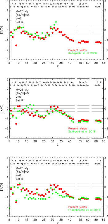
Figure 33. Comparison between the [X/O] produced by a nonrotating 25  star of solar metallicity and analogous yields provided by Kobayashi et al. (2006; upper panel), Sukhbold et al. (2016; middle panel), and Frischknecht et al. (2016; lower panel).
Download figure:
Standard image High-resolution imageThe comparison between our yields and the abundances published by Frischknecht et al. (2016) for rotating models is shown in Figure 34. It is important to note that the two models have not been computed with the same initial rotation velocity. In fact, while we fix the initial velocity (e.g., 150 or 300 km s−1) independent of the initial mass, Frischknecht et al. (2016) assume a given value of v/vcrit (e.g., 0.4 or 0.5), which obviously implies a different initial velocity for the various models. Nevertheless, our 25  model computed with vini = 300 km s−1 roughly corresponds to their model computed for v/vcrit = 0.4. The upper panel refers to the solar-metallicity case while the lower one to [Fe/H] = −1. In the solar-metallicity case, the main differences between the two models concern essentially the light s-process elements (the weak component) up to the neutron closure shell at n = 50. In particular, while these elements are coproduced with O in our models, they are substantially underproduced in Frischknecht et al. (2016). At low metallicity, on the contrary, the differences mainly concern the heavy elements above n = 50. In fact, these elements are produced in our model, while they are not produced at all in Frischknecht et al. (2016). In addition to this, F, Na, and Al are also largely overproduced with respect to O in their model. Again, we do not have any real explanation for these differences but we want to note again that the inclusion of rotation in an evolutionary code requires a calibration, and that different calibrations may even lead to very different results. It is worth noting, however, that even in the nonrotating models, at solar metallicity, where it is generally accepted that massive stars produce the weak component, the model of Frischknecht et al. (2016) shows a substantial underproduction of all these elements.

Figure 34. Upper panel: comparison between the [X/O] obtained after the explosion of a 25  star of solar metallicity rotating at 300 km s−1 and the pre-explosive yields obtained for the same mass by Frischknecht et al. (2016). Lower panel: same comparison but for [Fe/H] = −1.
Download figure:
Standard image High-resolution image7. Initial Mass–Remnant Mass Relation
The three different choices for the calibration of the explosions that we discussed above (sets F, M, and R) obviously imply different remnant masses. Figure 35 collects for set F the remnant masses for all metallicities and all initial rotational velocities. The figure clearly shows that the choice that all stars eject 0.07  of
of  does not allow the formation of remnants more massive than ∼9 M⊙. The same would occur even for lower amounts of
  , provided, however, that at least part of the nuclei produced by the explosive burning is ejected. It is also worth noting that for each mass, there is a spread of remnant masses despite the fact that all of them are obtained by requiring the ejection of the same amount of
  . Such a spread is largely reduced if the remnant masses are plotted versus the CO core mass (Figure 36). The reason is that, as already mentioned in this paper, the evolution of a star beyond the central He-burning phase is predominantly determined by the size of the CO core, irrespective of the initial rotational velocity and metallicity. The residual spread in Figure 36 is due to the fact that the advanced evolutionary phases are not just a function of the CO core mass but also of the amount of 12C left by core He burning, since it determines how much the C-burning shell may advance in mass before the final collapse. Though the relation depicted in Figure 36 may be used to get a good idea of the remnant masses, we strongly discourage any user from applying this relation to other models, different from the present ones, to infer any explosive yield. The reason is that the spread shown in this figure, though quite tight, is larger than the region where all explosive burning occurs (which amounts to a few tens of solar masses). The remnant masses obtained for set M do not differ significantly from those obtained for set F because, although we apply mixing and fallback for these models, the mixed zone is not very extended, and therefore the mass cuts needed to eject 0.07 M⊙ of
  are in any case deep enough and not very different from the ones obtained for set F.

Figure 35. Remnant masses obtained for set F as a function of the initial mass.
Download figure:
Standard image High-resolution image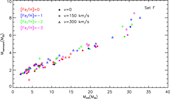
Figure 36. Remnant masses obtained for set F as a function of the CO core mass.
Download figure:
Standard image High-resolution imageSet R, on the contrary, is profoundly different from the previous ones because in this case, we assume that all stars more massive than 25  fully collapse. Obviously, in this case, the remnant masses are much larger than in the previous cases (see Figure 37), and some of the masses larger than 25 M⊙ leave black hole remnants even much larger than those associated with the detections of the gravitational waves GW 150914, GW 151226, GW 170104, GW 170608, and GW 170814 (Abbott et al. 2016a, 2016b, 2016c, 2017a, 2017b, 2017c). Though this result could be considered quite trivial and obtained "by construction," Figure 37 shows some interesting features. At solar metallicity, the maximum remnant mass that can be formed is ∼30 M⊙, irrespective of the initial rotational velocity (at least up to 300 km s−1). The reason is that at solar metallicity, mass loss is efficient enough that the final mass of all these models is lower than ∼30 M⊙. At lower metallicities, the strong reduction in the mass loss allows the nonrotating models to form much larger remnant masses. In rotating models, on the contrary, the remnants are on average much smaller because rotation pushes many stars above their Eddington luminosity where they lose much more mass than their nonrotating counterparts.

Figure 37. Remnant masses obtained for set R as a function of the initial mass.
Download figure:
Standard image High-resolution image8. Summary and Conclusions
In this paper, we presented a new very extended set of models and yields of massive stars in the range 13–120 M⊙, initial metallicities [Fe/H] = 0, −1, −2, and −3, and initial rotation velocities v = 0, 150, and 300 km s−1. All of the models were followed from the pre-main-sequence up to the presupernova stage. The explosion was simulated artificially by means of a hydrodynamic code in the framework of a kinetic bomb, and the computation of the explosive nucleosynthesis is fully coupled to the hydrodynamics. Given the arbitrariness in the calibration of the explosion, we discussed three different choices for this calibration, and we showed how the yields and the masses of the remnants depend on the adopted choice. We took into account a large nuclear network, fully coupled to the stellar evolution, that extends from neutrons to 209Bi, explicitly including 335 nuclear species and more than 3000 nuclear reactions. The efficiency of the rotation-induced mixing was calibrated by requiring the fit to a subset of stars (taken from the LMC samples of the FLAMES survey; Hunter et al. 2009) for which both the surface N abundance and the projected rotation velocity are available. Most of the properties of this grid of models, together with the final yields, are available for download from the Web site http://orfeo.iaps.inaf.it. More specific details about the models and/or the explosions may be obtained upon request.
A synthesis of the surface properties of all our models is shown in Figure 38, and it helps in visualizing what is described in the remainder of this section.

Figure 38. Global properties of all the models as a function of mass, metallicity, and initial rotation velocity. Each bar represents, for each model, the configuration of the star as a function of the fraction of time remaining to final collapse after core H depletion. The colors refer to the RSG (red), BSG (blue), and WR (green) configurations, respectively. The expected supernova type is reported on top of each bar: orange refers to SNIIP and black to SNIb. Stars expected to enter the pulsation pair instability regime are marked by a hatched black square. For each stellar model, the final remnant masses are shown by filled circles for set F, and by crosses, for set R.
Download figure:
Standard image High-resolution image
At solar metallicity, nonrotating stars populate the RSG branch up to a luminosity log(L/L⊙) ∼ 5.7, which corresponds to a mass of ∼40 M⊙. More massive stars lose a major fraction of their H-rich envelope because they overcome their Eddington luminosity before reaching the RSG branch and hence turn back blueward, where they spend all their He-burning lifetime. Stars more massive than ∼20 M⊙ leave the RSG branch sometime during the core He-burning phase and evolve toward a BSG configuration, eventually becoming WR stars (MWR ∼ 20 M⊙). Accordingly, the maximum mass we predict for the progenitors of SNIIP is MIIP ∼ 17 M⊙ (which corresponds to a maximum luminosity of log(L/L⊙) ∼ 5.1). Stars with M > MIIP are expected to explode as SNIb. By the way, because our grid does not have enough resolution in the initial mass, and therefore in the final H envelope mass, we cannot clearly define the transition SNIIP/SNIIb/SNIb according to Hachinger et al. (2012); therefore, we choose for the moment to consider only two limits, i.e., SNIIP and SNIb, also because from the observational side, the classification is not yet very clear. The properties of these models are in reasonable agreement with some observed properties of the massive stars: (a) the predicted distribution of the stars in the HR diagram is compatible (both in luminosity and effective temperature) with the distribution observed in a sample of the galactic RSG stars (Levesque et al. 2005); (b) the maximum mass exploding as SNIIP is compatible with the lack of detected progenitors (of SNIIP) with luminosities higher than log(L/L⊙) ∼ 5.1, as reported by Smartt (2009, 2015), and therefore, our scenario naturally explains the so-called "RSG problem" (Smartt 2009)—note however that other hypotheses to solve this problem are provided, e.g., by Walmswell & Eldridge (2012) and Yoon & Cantiello (2010); (c) in a scenario in which all of the stars with M > 25 M⊙ fail to explode and collapse directly to a black hole, we do not expect SNIb at luminosities larger than log(L/L⊙) ∼ 5.6. This result is at least not in contradiction with the 14 SNIb progenitors with no detection reported by Smartt (2015); moreover, the expected amount of mass ejected by stars exploding as SNIb is of the order of Mejecta ∼ 6 M⊙, in rather good agreement with the ejected masses of 3–4 M⊙ estimated from the SNIb light curve fitting (Wheeler & Levreault 1985; Ensman & Woosley 1988; Dessart et al. 2011, 2015, 2016; Lyman et al. 2016); and (d) a limiting mass between SNIIP and SNIb corresponding to MIIP ∼ 17 M⊙ implies a fraction of SNIb of ∼26% of all core-collapse supernovae (CCSNe; having assumed a Salpeter IMF, a minimum mass for the CCSNe of ∼9.5 M⊙, and an upper mass limit Mtop ∼ 25 M⊙): this number is in very good agreement with the SN rates estimated from the volume-limited Lick Observatory Supernova Search (LOSS; Smith et al. 2011).
Rotation completely changes this scenario because it lowers both the maximum mass that spends a substantial amount of time on the RSG branch and the minimum mass that becomes a WR. In particular, we get that even the 13  rotating at either 150 and 300 km s−1 becomes a WR star. The maximum mass that reaches the RSG branch decreases to 30
  for v = 150 km s−1 and to 25
  for v = 300 km s−1. Therefore, we predict that solar-metallicity models, with initial rotation velocities v ≥ 150 km s−1, explode as SNIb (MIb ≲ 13 M⊙) and that RSG stars are expected up to a luminosity of the order of log(L/L⊙) ∼ 5.5.
At [Fe/H] = −1, in the absence of rotation, the strong decrease of the mass loss (coupled to the strong reduction of the opacity) increases the maximum mass that settles on the RSG branch up to 25–30,  but it also prevents the more massive ones from reaching the RSG branch before explosion, because these stars turn toward their Hayashi track on a nuclear timescale. Hence, we expect RSG SNIIP progenitors with masses as high as MIIP ∼ 25–30 M⊙ and those above this value explode as BSG SNIIP. Given the very small amount of mass lost at this metallicity, WR stars may form only at masses M ≥ 80 M⊙. At lower metallicities ([Fe/H] ≤ −2), the less massive stars also turn to the red on a nuclear timescale, so that basically no stars are expected to populate significantly the RSG branch at these metallicities. This does not imply that we do not expect RSG SNIIP because stars in the range 13 to 25
  reach the RSG branch toward the end of the central He-burning phase. Given the extremely small amount of mass lost by these stars, all of them explode as SNIIP (BSGs or RSGs).
The main role of rotation at these metallicities is that of pushing the stars toward the RSG branch. As a consequence, stars below 25–30  now spend a considerable amount of time on the RSG branch where they eventually explode as RSGs (SNIIP) while the more massive ones approach their Eddington luminosity when their surface temperature drops to
  ∼ 3.8–4.0, lose a huge amount of mass, and turn to the blue, becoming WR stars. So at subsolar metallicities rotation populates the RSG branch up to 25–30 M⊙, leads to the formation of WR stars in a quite wide range of masses, and settles a limiting mass between SNIIP and SNIb in the range MIIP 25—30M⊙. Though up to now no progenitor for SNIIP as massive as 25–30 M⊙ has been detected yet, the present results imply the existence of these massive RSG progenitors (and SNIIP) at low metallicities, and we certainly expect such a finding in the next future.
Before closing this part, it is important to stress that since stars do not rotate at the same rotation velocity (as seen from the available observational data) but show a spread of values, the choice of an IDROV (Initial Distribution of ROtation Velocities) is mandatory (as the IMF for the mass distribution) when trying to fit the properties of a given sample of stars or a trend with the metallicity (Prantzos et al. 2018, CL13). In the presence of a spread of initial rotation velocities, even the definition of a limiting mass becomes much more ambiguous because it depends not just on the metallicity but also on Vini. A detailed and quantitative analysis of the properties of a population of massive stars, where both the IMF and the IDROV are taken into account, is beyond the scope of the present paper and will be addressed in a future work.
The direct detections of gravitational waves, GW 150914, GW 151226, GW 170104, GW 170608, and GW 170814 (Abbott et al. 2016a, 2016b, 2016c, 2017a, 2017b, 2017c) have been associated with the merger of two black holes, presumably of stellar origin, GW 150914 and GW 170608, which are considered the largest (∼29–36 M⊙) and smallest (∼7–12 M⊙) black holes in a binary system, respectively. In a scenario in which all stars eject 0.07 M⊙ of 56Ni, the maximum mass of the remnant ranges between ∼4 M⊙ and ∼8 M⊙, for −3 ≤ [Fe/H] ≤ 0 and 0 ≤ vini ≤ 300 km s−1. In the alternative scenario in which all stars with M > 25 M⊙ fail to explode and directly collapse into a black hole, the remnant masses are obviously much larger and can reach values as high as ∼80 M⊙ for low-metallicity, nonrotating models. In this paper, we just wanted to show that, in principle, a black hole with a mass as large as ∼80 M⊙ can be obtained as the final product of the evolution of a single massive star, without any claim on the route toward the formation of the black hole binary system as well as their merging (Antonini & Rasio 2016; Belczynski et al. 2016; Mandel & de Mink 2016). Of course, such a result may change, even significantly, if the massive star evolves in a binary system (de Mink & Mandel 2016). A natural upper limit to the maximum mass of a (stellar) black hole is given by the fact that stars above a given critical mass (MPISN) enter the pair instability regime and explode as PISNe without leaving any remnant. In general, MPISN decreases with increasing initial rotation velocity because of the substantial increase of the CO core induced by the rotation-driven mixing so that rotation favors the formation of a PISN.
As far as the final yields are concerned, our current preferred scenario (set R) is obtained by requiring that stars in the range 13 to 25  experience mixing and fall back (Umeda & Nomoto 2002; the inner and outer borders of the mixed region are fixed by imposing that [Ni/Fe] = 0.2 and that it cannot extend beyond the base of the oxygen shell) and then the mass cut is fixed by requiring the ejection of 0.07
  of
of  . Stars more massive than 25
  are assumed to fully collapse in the remnant so that they contribute to the yields only through their wind. The same choices were assumed for all metallicities and initial rotation velocities. The overall behavior of the yields provided by the nonrotating models is basically the expected one. At solar metallicity, the PFs of the intermediate-mass nuclei show a reasonably flat profile; the elements between Zn and Zr are also produced by the so-called weak component. Elements beyond the neutron closure shell n = 50 are not produced at all. As the metallicity decreases, the PFs of the intermediate-mass even particle remain quite flat (because of their primary origin) and close to that of O, while the odd nuclei show a progressively more pronounced odd–even effect. Elements beyond Zn are not produced at all, as well as N and F, which are also severely underproduced.
The most striking effect of rotation on the yields is the substantial production of N, F, and all elements heavier than Fe up to Pb in the low-metallicity models. Conversely, at solar metallicity, the influence of rotation on the yields is modest (at least up to Vini = 300 km s−1). The continuous stirring of matter between the central He-burning and the H-burning shell leads to the high production of the CNO cycle (and obviously  which is the most abundant) that are then redistributed within the He core. The fraction of these nuclei that falls in the convective core is rapidly nuclearly processed, and in particular
  is converted to
  , i.e., a powerful primary neutron source. Another fraction of these nuclei remains frozen in the radiative part of the He core and becomes the fuel that powers the synthesis of F when the He convective shell forms after the central He-exhaustion phase. The capability of matter to flux beyond the two neutron closure shells at n = 50 and n = 82 depends basically on the neutron to seed ratio because this is the quantity that controls the timescale necessary to overcome the neutron closure shells. A natural limit to the maximum overproduction of the heavy elements is obviously given by the total amount of matter that may be pushed onward, and obviously this is the total amount of Fe available. Our rotating models raise the neutron to seed ratio above 1000, a value that is more than enough to allow the passage of matter through the neutron closure shell in a timescale much shorter than the lifetimes of the stars in He burning (see, e.g., Figures 7–22 in Clayton 1968). Hence, our models are able to produce efficiently nuclei up to Pb. The production factors of the heavy nuclei, however, reaches the maximum at [Fe/H] = −1 and then drops slightly, the obvious explanation being that the lower the metallicity, the lower the availability of target nuclei, i.e., Fe.
The final yields are the results of the computation of a large number of models from the pre-main-sequence to core collapse plus the explosion. All these computations are, however, based on a large number of assumptions and choices that may vary from author to author. In order to check if these yields are capable of fitting the solar distribution as well as their observed trend with the metallicity, we already included them in a galactic chemical evolution model (Prantzos et al. 2018), and we strongly refer the reader to that paper to have an idea of how these yields behave. Here we want just to point out that in that paper, we calibrated the IDROVs by requiring a primary-like behavior of 14N in the Milky Way at low metallicity, at the same time the overproduction of s-process elements at intermediate metallicities. The next step in this endless attempt to produce scenarios increasingly closer to reality will be the extension of the grid to zero metallicity and super metal-rich stars.
M.L. warmly thanks Francesca Primas and Ferdinando Patat for their generous hospitality during his visit at ESO and acknowledges the support by the ESO Visitor Program 2017–2018. This work has been partially supported by the Italian grants "Premiale 2015 MITiC" (P.I. B. Garilli) and "Premiale 2015 FIGARO" (P.I. G. Gemme).
Appendix: The FRANEC Code
In this section, we recall briefly all of the main features and input physics of our evolutionary code (FRANEC), already presented in detail in CL13.
The set of equations describing the physical structure of the star plus the ones governing the chemical evolution of the chemical composition (i.e., the local burning due to the nuclear reactions plus the various kinds of mixing: convection, semiconvection, and rotationally induced mixing) are coupled together and solved simultaneously by means of a relaxation technique. The angular momentum transport, together with the determination of the velocity of the meridional circulation, is solved separately, again by means of a relaxation technique.
The borders of the convective zones are defined according to the Ledoux criterion. In addition, we assume 0.2HP of overshooting at the outer edge of the convective core only during the core H-burning phase.
The equation of state (EoS) adopted for temperatures lower than 106 K is the one provided by Rogers et al. (1996) and Rogers (2001; EOS and ESOPLUS). For temperatures higher than 106 K, we used the EoS tables given by Straniero (1988).
The radiative opacity coefficients are derived from Kurucz (1991) for T ≤ 104 K, from Iglesias et al. (1992) for 104 < T (K) ≤ 108 (OPAL), and from the Los Alamos Opacity Library (LAOL) Huebner et al. (1977) for 108 < T (K) ≤ 1010. The opacity coefficients due to thermal conductivity are derived from Itoh et al. (1983).
Mass loss has been included following the prescriptions of Vink et al. (2000, 2001) for the BSG phase (Teff > 12,000 K), de Jager et al. (1988) for the RSG phase (Teff < 12,000 K), and Nugis & Lamers (2000) for the WR phase. The enhancement of mass loss due to the formation of dust during the RSG phase has been included following the prescriptions of van Loon et al. (2005). Mass loss is enhanced, in rotating models, following the prescription of Heger et al. (2000).
The criteria adopted to define the different WR subclasses are the same as those adopted in Limongi & Chieffi (2006), i.e., we assume that the star enters the WR phase when log Teff > 4 and Hsurf < 0.4, and we adopt the following usual definitions for the various WR phases: WNL (10−5 < Hsurf < 0.4), WNE [Hsurf < 10−5 and (C/N)surf < 0.1], WNC [0.1 < (C/N)surf < 10], and WCO [(C/N)surf > 10].
The nuclear network and the cross-section adopted have been discussed and presented in detail in the text (see Tables 1, 3, and 4).
The effect of rotation on the structure of the star has been included following the "shellular rotation" approach (Zahn 1992; Meynet & Maeder 1997). The transport of angular momentum due to meridional circulation and shear turbulence has been treated by means of the advective–diffusive equation (Chaboyer & Zahn 1992; Talon et al. 1997),
where U is the radial component of the velocity of the meridional circulation, Ds.i. the diffusion coefficient for the shear turbulence, and all other quantities have their usual meaning. We adopted the prescription for U provided by Maeder & Zahn (1998; their Equation (4.38)) and the formulation of Ds.i. proposed by Talon & Zahn (1997), modified later by Palacios et al. (2003):

where  ,
,  , and
, and  . Dh is the coefficient of horizontal turbulence that we assume (Zahn 1992):

where  is the thermal diffusivity (Meynet & Maeder 2000). The adoption of the expression for the velocity of the meridional circulation provided by Maeder & Zahn (1998) in Equation (1) leads to a fourth-order partial differential equation that is solved by means of a relaxation technique. In contrast, the transport of the chemical species has been treated as a pure diffusive process according to Chaboyer & Zahn (1992). In this case, the diffusion coefficient is given by

where Ds.i. is given by Equation (2), while Dm.c. is

as suggested by Zahn (1992).
The calibration of the mixing efficiency has been performed by means of two free parameters, namely, fc and fμ. The first free parameter, fc, simply multiplies the total diffusion coefficient defined in Equation (4) and is adopted for the mixing of the chemical composition, i.e.,

The second free parameter, fmu, multiplies the gradient of molecular weight, i.e.,  , and regulates the influence of this quantity on the mixing of both the angular momentum and the chemical composition. The calibration procedure is described in detail in the text (Section 3).
As usual, the initial He abundance and the mixing-length parameters have been determined by fitting the present properties of the Sun.