


Abstract
Linelists and radiative cooling functions in the local thermodynamic equilibrium limit have been computed for the six most important isotopologues of lithium hydride, 7LiH, 6LiH, 7LiD, 6LiD, 7LiT, and 6LiT. The data are based on the most accurate dipole moment and potential energy curves presently available, the latter including adiabatic and leading relativistic corrections. Distance-dependent reduced vibrational masses are used to account for non-adiabatic corrections of the rovibrational energy levels. Even for 7LiH, for which linelists have been reported previously, the present linelist is more accurate. Among all isotopologues, 7LiH and 6LiH are the best coolants, as shown by the radiative cooling functions.
Export citation and abstract BibTeX RIS
1. Introduction
The first small molecules formed after the Big Bang are presently considered to be the main actors in the cooling of primordial clouds, through their rovibrational transitions (Miller et al. 2010). The large abundance of H2 and  makes them natural candidates to have headed the cooling process (Abel et al. 2002), but due to the absence of a permanent electrical dipole moment, cooling is not very effective. At low temperatures, and in the presence of sufficient deuterium, H/D exchange occurs, which is essentially a reduced mass effect, since HD vibrational levels have a lower energy than the corresponding H2 levels. There would then be an overabundance of deuterated molecules (Galli & Palla 1998). Consequently, the cooling properties of the deuterated isotopologues, HD and HD+ (with very small isotopic dipole moments, however) have been investigated (see Coppola et al. 2011, Ripamonti 2007, and references therein) and it was concluded that HD is a much better coolant than H2 and can cool gases to temperatures below 200 K. Indeed, electric dipole (E1) transitions, with angular momentum selection rules ΔJ = ±1, are possible for the deuterated isotopologues, but not for H2 or
  , for which rotational states must have either even or odd J, depending on the nuclear spin. For ortho (triplet) nuclear spin, J must be odd, and for para (singlet) nuclear spin it must be even, so that only quadrupole transitions (E2 or M2), with selection rules ΔJ = ±2, are feasible.
LiH isotopologues and related ions were less abundant, but have, on the other hand, much larger (7000 times that of HD) regular dipole moments, which yields intense pure rotational and rovibrational transitions. It has been suggested that Li, mainly the 7Li nucleid, was formed a few minutes after the lighter atoms, thus LiH and LiH+, formed soon after, are now also being considered to have played a role in the cooling process, at temperatures of up to 5000 K (Stancil et al. 1996; Bougleux & Galli 1997; Galli & Palla 1998; Bovino et al. 2011).
Although fractional abundances and a study of kinetic routes for isotopologues other than 7LiH are still missing, one could speculate that if there was sufficient deuterium, D, in order for HD to play a role in the cooling, so could LiD. This hypothesis has never been considered, however, at least not in accurate calculations. A possible explanation is that while HD introduces the dipole moment component compared to H2, the variation of the LiH dipole moment when passing from LiH to LiD (lowered by 0.01 Debye (Wharton et al. 1962)) appears to be irrelevant. However, the number of bound states of LiH and LiD are very different, as well as their transition energies. Furthermore, changes of the nuclear mass also affect the rovibrational energy levels that can possibly be accessed, mainly through inertial effects, but also through small adiabatic and non-adiabatic shifts, which deserves investigation. This also applies to the isotopologues containing the 6Li nucleus. 6Li was less abundant in the early universe than 7Li, by one or two orders of magnitude according to standard Big Bang Nucleosynthesis theory, though there might have been much more of it than this theory suggests (Jedamzik 2008; Kusakabe et al. 2013; Anders et al. 2014; Mukhamedzhanov et al. 2016). Full and accurate linelists for all isotopologues of LiH are therefore desirable for future work.
In theoretical models and calculations, the cooling capacity is described by the so-called radiative cooling function, which gives the molecular average rate of energy loss at a given temperature (Hollenbach & McKee 1979; Galli & Palla 1998). Energy loss can be due to collisional or radiative de-excitation. If the density is higher than the critical density (see Equation (2) of Coppola et al. 2011), local thermodynamic equilibrium (LTE) prevails, and collisions dominate the de-excitation process. In this limit, cooling is achieved essentially by rovibrational molecular transitions. The evaluation of the radiative cooling function requires accurate linelists and dipole moment curves (DMCs). It has already been computed for the 7LiH isotopologue by Coppola et al. (2011) and by Shi et al. (2013) in the temperature range of 10–104 K.
These two works report state-of-the-art rovibrational linelists for 7LiH, but are not in full accordance, diverging in the lower and higher temperature limits, as we will discuss in the present work. Coppola et al., in their linelist published in 2011, use their own potential energy curve (PEC), with which the rovibrational energy values were obtained, as well as their own DMC, both obtained with internally contracted multi-reference averaged-pair functional calculations. In the more recent (2013) linelist by Shi et al., as compared to the previous work, the authors resort to a arguably more accurate empirical PEC from Coxon & Dickinson (2004) but a less accurate theoretical DMC from Partridge & Langhoff (1981). Recently, extremely accurate potential energy and DMCs have been published, which make a new evaluation of the cooling functions desirable.
The first accurate PEC is due to Holka et al. (2011), who employed the MR-CISD (multi-reference configuration- interaction singles-doubles) method with the cc-pwCV5Z basis set and added relativistic and diagonal adiabatic corrections. Non-adiabatic effects on the computed vibrational energies were treated explicitly using the Bunker & Moss (1977) formalism. The second accurate PEC was achieved by Tung et al. (2011), obtained with all-particle explicitly correlated Gaussian functions with shifted centers and containing adiabatic diagonal Born–Oppenheimer corrections (DBOCs). Atomic masses were used in the vibrational calculations to to simulate non-adiabatic vibrational shifts. Compared with experimental data, the vibrational energies obtained by the two groups differ by 1–2  . In a more recent work (Diniz et al. 2016), we once again used the all-particle explicitly correlated Gaussian functions with shifted centers approach to obtain a very accurate DMC, and computed the rovibrational spectrum and transition probabilities for 7LiH. In these calculations, non-adiabatic effects on the energy levels and on the dipole moment are simulated through an R-dependent (R being the nuclear distance) reduced mass, introduced previously by our group (Diniz et al. 2015). Such a treatment improves the accuracy of the vibrational energies by one order of magnitude.
In the present work we apply our approach in order to assess and surpass the differences between the two available linelists, concerning the energy spectrum, transition probabilities, and cooling function. We then present for the first time (a) complete linelists and (b) radiative cooling functions (in the LTE limit) also for the other isotopologues, namely 6LiH, 7LiD, 6LiD, 7LiT, and 6LiT. The compounds with tritium (T) are included for the sake of completeness. In Section 2 the basic theory and equations are developed. In Section 3 the vibrational energies are provided and the effect of the choice of reduced mass is discussed, while the linelists are presented in Section 4. Section 5 is devoted to the evaluation of the cooling functions for all isotopologues and a discussion of the new features introduced here, including the non-adiabatic corrections. Section 6 concludes this article.
2. Theory and Details of the Calculations
In the electronic one-state approximation, Schrödinger's radial equation for a diatomic molecule is (Bunker & Moss 1977)
where R is the internuclear distance, μv and μr are, respectively, the vibrational and rotational reduced masses, Ee(R) is the PEC, and EvJ and χvJ are the eigenvalues and rovibrational wavefunctions of the quantum state characterized by the vibrational and rotational quantum numbers v and J. Within the common Born–Oppenheimer and adiabatic approximations, the masses μv and μr are the same and equal to the reduced mass of the nuclei. Solving this equation for the rovibrational functions and employing the DMC, d(R), the Einstein A coefficients, or dipole transition probabilities, can be calculated as
where
is the Hönl–London rotational intensity factor, and ν is the transition frequency. In the LTE limit, the radiative cooling function is given by (see Coppola et al. 2011)
In the above equation, the symbols (v', J') and (v'', J'') denote, respectively, the upper and lower rovibrational states between which a spontaneous transition may occur. In highly accurate calculations, DBOC and relativistic corrections are typically added to the Born–Oppenheimer PEC before solving Equation (1). Non-adiabatic corrections, on the other hand, are dynamical corrections and can be simulated by judicious choice of the masses μv and μr, as will be explained below.
In our calculations, we used the very accurate adiabatic PEC of Tung et al. (2011), which comprises the Born–Oppenheimer energies together with the DBOC. To this curve, we added the leading relativistic correction reported by Holka et al. (2011). Rovibrational states were computed with our own renormalized Numerov code where allowance was made for coordinate-dependent reduced masses (Alijah & Duxbury 1990). The numerical integration was performed within the range of 1.2 a0 ≤ R ≤ 30.0 a0, and parameters were controlled to achieve numerical convergence to 10−14 Eh. Extension of the potential at small distances was found to be necessary to obtain well converged results for the highest vibrational states. To this end, the data points of the interval between 1.8 and 2.5 a0 were fitted to the expression f(R) = a + b exp(cR). For all isotopologues, b = (7.8 ± 0.4) Eh and c = (−2.26 ± 0.03) a0−1, while a (within ±0.0009 Eh) is −8.0852 Eh for  ,
,  for
for  , −8.0851 Eh for 6LiH, −8.0852 Eh for 6LiD, −8.0854 Eh for 7LiT, and −8.0853 Eh for 6LiT.
The present (X1Σ+) PEC has an equilibrium distance of r0 = 3.015 a0 and a dissociation energy of De = 20287.6  , in very good accordance with the experimental values of Stwalley & Zemke (1993), namely r0 = 3.015 a0 and De = 20287.7
  . For comparison, the PEC used by Coppola et al. (2011) has r0 = 3.014 a0 and De = 20294
  , the latter with an estimated uncertainty of ±15
  . Comparing with the "exact BO" dissociation energy (without adiabatic and relativistic corrections) of Cooper & Dickinson (2009), De = 20298.8
  , Coppola et al. report 20305
  , while we found an exact match, 20298.8
  , with our PEC. It becomes clear that the present PEC is superior. Shi et al. (2013) resort to an empirical (supposed exact) PEC in the range 2 < R < 20 a0, and for smaller and higher values of R, they use extrapolation formulae. Curiously, they were not able to obtain the higher (v = 23, J = 0) state obtained by Coppola et al. (which we also obtained; see Section 3).
In the calculation of transition probabilities and related quantities, we used our very accurate DMC (Diniz et al. 2016). Figure 1 of this reference shows the differences between our DMC and those used by Coppola et al. (2011) and Shi et al. (2013) for their respective linelists. The present DMC was also obtained with all-particle explicitly correlated Gaussian functions with shifted centers. We can conclude, in consequence, that it is more accurate than that used by Shi et al. and should generate superior Einstein coefficients. In Figure 1 and Table 6, discussed in Section 4, we present the Av'J'v''J'' coefficients for the three cases.

Figure 1. Comparisons of the Einstein A coefficients for the (1−0) band of the 7LiH.
Download figure:
Standard image High-resolution imageApproximate non-adiabatic corrections can be introduced by employing, for μv, atomic, instead of nuclear, reduced masses in Equation (1). However, effective R-dependent reduced masses perform much better (Kutzelnigg 2007). Rotational non-adiabatic effects, on the other hand, are much less pronounced. A good procedure for many states is therefore to keep the nuclear masses for μr. Based on the excellent performance of the effective vibrational mass from Diniz et al. (2015) for the 7LiH isotopologue, we kept this approach for the other isotopologues, which means using a R-dependent vibrational reduced mass μv and the constant nuclear reduced mass for μr. Calculations with simply atomic and nuclear reduced masses have also been performed for comparison.
3. Vibrational Energies
We have calculated the vibrational energies for six isotopologues of lithium hydride. In Figure 3 of a previous publication (Diniz et al. 2015) we demonstrated that our computed vibrational energies for 7LiH agree with experimental data reported by Coxon & Dickinson (2004) to better than 0.2  for states up to v = 15. For higher states, the deviation increases to up to 1
  . As discussed in that earlier paper, these states are close to the avoided crossing region between the two lowest electronic states, which makes their description within a one-state picture very demanding. Furthermore, Coxon and Dickinson's data begin to deviate from those of the previous compilation of experimental data by Chan et al. (1986). They were weighted lower in their empirical fitting procedure.
In the present paper we report a full comparison with experimental data in Table 1. In view of the experimental uncertainties, two sets of root mean square values are presented for a useful comparison: the first, denoted rms, includes all experimental states, while the second, denoted rms*, only refers to states with v < vc, the vibrational state above which the experimental energies from Coxon & Dickinson (2004) and Chan et al. (1986) disagree by more than 0.1  (for example, vc = 15 for 7LiH). Comparison is made with ab initio calculations by Holka et al. (2011; HOLKA), Coppola et al. (2011; COPPOLA) and that by Shi et al. (2013; SHI). Our data (EFF) show approximately the same rms* as SHI, 0.1
  , while HOLKA and COPPOLA present differences of 2
  and 6
and 6  , respectively.
Table 1. 7LiH—Comparison of Calculated and Experimental Vibrational Term Values

|
HOLKA | Δ(a) | Δ(b) | COPPOLA | Δ(a) | Δ(b) | SHI | Δ(a) | Δ(b) | EFF | Δ(a) | Δ(b) |
|---|---|---|---|---|---|---|---|---|---|---|---|---|
| 1–0 | 1360.58 | 0.87 | 0.87 | 1360.48 | 0.77 | 0.77 | 1359.71 | 0.00 | −0.00 | 1359.68 | −0.02 | −0.03 |
| 2–0 | 2676.11 | 1.55 | 1.51 | 2676.07 | 1.51 | 1.47 | 2674.56 | 0.00 | −0.04 | 2674.50 | −0.06 | −0.10 |
| 3–0 | 3947.53 | 2.06 | 2.04 | 3947.70 | 2.23 | 2.21 | 3945.47 | 0.00 | −0.02 | 3945.39 | −0.08 | −0.10 |
| 4–0 | 5175.69 | 2.41 | 2.43 | 5176.23 | 2.95 | 2.97 | 5173.28 | 0.00 | 0.02 | 5173.19 | −0.09 | −0.07 |
| 5–0 | 6361.35 | 2.62 | 2.65 | 6362.41 | 3.68 | 3.71 | 6358.73 | 0.00 | 0.03 | 6358.63 | −0.10 | −0.07 |
| 6–0 | 7505.19 | 2.72 | 2.72 | 7506.88 | 4.41 | 4.41 | 7502.48 | 0.01 | 0.01 | 7502.37 | −0.11 | −0.10 |
| 7–0 | 8607.73 | 2.70 | 2.66 | 8610.17 | 5.14 | 5.10 | 8605.05 | 0.01 | −0.02 | 8604.93 | −0.10 | −0.14 |
| 8–0 | 9669.38 | 2.58 | 2.53 | 9672.66 | 5.86 | 5.81 | 9666.82 | 0.02 | −0.03 | 9666.72 | −0.08 | −0.13 |
| 9–0 | 10690.35 | 2.39 | 2.33 | 10694.52 | 6.56 | 6.50 | 10688.00 | 0.04 | −0.02 | 10687.91 | −0.05 | −0.11 |
| 10–0 | 11670.64 | 2.12 | 2.10 | 11675.73 | 7.21 | 7.19 | 11668.59 | 0.06 | 0.05 | 11668.51 | −0.02 | −0.03 |
| 11–0 | 12610.00 | 1.82 | 1.84 | 12615.98 | 7.80 | 7.82 | 12608.28 | 0.10 | 0.12 | 12608.20 | 0.01 | 0.04 |
| 12–0 | 13507.79 | 1.50 | 1.54 | 13514.61 | 8.32 | 8.36 | 13506.44 | 0.15 | 0.19 | 13506.34 | 0.05 | 0.09 |
| 13–0 | 14362.96 | 1.21 | 1.23 | 14370.51 | 8.76 | 8.78 | 14361.96 | 0.21 | 0.23 | 14361.89 | 0.14 | 0.16 |
| 14–0 | 15173.83 | 0.96 | 0.91 | 15181.99 | 9.12 | 9.07 | 15173.14 | 0.28 | 0.22 | 15173.13 | 0.27 | 0.21 |
| 15–0 | 15938.00 | 0.80 | 0.64 | 15946.60 | 9.40 | 9.24 | 15937.55 | 0.36 | 0.19 | 15937.65 | 0.45 | 0.29 |
| 16–0 | 16652.03 | 0.70 | 0.45 | 16660.89 | 9.56 | 9.31 | 16651.76 | 0.44 | 0.18 | 16652.02 | 0.69 | 0.44 |
| 17–0 | 17311.21 | 0.64 | 0.36 | 17320.10 | 9.53 | 9.25 | 17311.08 | 0.51 | 0.23 | 17311.45 | 0.88 | 0.60 |
| 18–0 | 17909.13 | 0.61 | 0.39 | 17917.77 | 9.24 | 9.03 | 17909.09 | 0.57 | 0.35 | 17909.38 | 0.86 | 0.64 |
| 19–0 | 18437.20 | 0.71 | 0.55 | 18445.26 | 8.77 | 8.61 | 18437.08 | 0.59 | 0.43 | 18437.25 | 0.76 | 0.60 |
| 20–0 | 18884.19 | 1.44 | 0.93 | 18891.32 | 8.57 | 8.06 | 18883.31 | 0.56 | 0.05 | 18883.84 | 1.09 | 0.58 |
| 21–0 | 19236.07 | ⋯ | 1.82 | 19241.72 | ⋯ | 7.47 | 19233.16 | ⋯ | −1.09 | 19234.51 | ⋯ | 0.26 |
| 22–0 | 19476.21 | ⋯ | 4.25 | 19479.53 | ⋯ | 7.57 | 19472.72 | ⋯ | 0.76 | 19472.63 | ⋯ | 0.67 |
| 23–0 | 19587.95 | ⋯ | ⋯ | 19581.61 | ⋯ | ⋯ | ||||||
| rms | 1.79 | 1.94 | 7.08 | 7.02 | 0.29 | 0.33 | 0.45 | 0.33 | ||||
| rms* | 2.06 | 2.05 | 5.95 | 5.94 | 0.11 | 0.11 | 0.10 | 0.11 | ||||
Note. EFF: term values are calculated in the present paper with the use of our effective mass obtained from a multi-structure valence bond approach (Diniz et al. 2015). HOLKA, SHI, and COPPOLA are the calculated term values by Holka et al. (2011, using the Bunker–Moss formalism), by Coppola et al. (2011), and by Shi et al. (2013), respectively. The Δ columns contain the differences between calculated and experimentally derived term values due to Coxon & Dickinson (2004), Δ(a), and due to Chan et al. (1986), Δ(b). All data are in wavenumbers,  .
.
Download table as: ASCIITypeset image
The vibrational energies of the other three stable isotopologues, 6LiH, 7LiD, and 6LiD, have now also been calculated and are shown in Tables 2, 3, and 4, respectively. Results obtained with reduced nuclear (NU) and atomic masses (AT) are included to demonstrate the improvement of the computed data due to the use of the effective mass. Since Shi et al. and Coppola et al. do not report results for these isotopologues, our values are compared only with the data of Holka et al. The predictions for the two long-lived isotopologues, 7LiT and 6LiT, for which no experimental data and theoretical calculations appear to be available, are presented in Table 5. The accuracy of our predictions is expected to be similar to that obtained for the most prominent isotopologue, 7LiH.
Table 2. 6LiH—Comparison of Calculated and Experimental Vibrational Term Values

|
NU | Δ(a) | Δ(b) | HOLKA | Δ(a) | Δ(b) | AT | Δ(a) | Δ(b) | EFF | Δ(a) | Δ(b) |
|---|---|---|---|---|---|---|---|---|---|---|---|---|
| 1–0 | 1373.83 | 0.46 | 0.46 | 1374.24 | 0.87 | 0.87 | 1373.49 | 0.13 | 0.12 | 1373.34 | −0.03 | −0.03 |
| 2–0 | 2701.83 | 0.88 | 0.83 | 2702.53 | 1.58 | 1.53 | 2701.19 | 0.23 | 0.19 | 2700.89 | −0.07 | −0.11 |
| 3–0 | 3984.98 | 1.28 | 1.25 | 3985.81 | 2.11 | 2.08 | 3984.05 | 0.34 | 0.32 | 3983.62 | −0.09 | −0.11 |
| 4–0 | 5224.13 | 1.65 | 1.66 | 5224.96 | 2.48 | 2.49 | 5222.93 | 0.45 | 0.46 | 5222.38 | −0.09 | −0.09 |
| 5–0 | 6420.05 | 2.01 | 2.01 | 6420.76 | 2.72 | 2.72 | 6418.60 | 0.56 | 0.56 | 6417.94 | −0.11 | −0.10 |
| 6–0 | 7573.39 | 2.32 | 2.31 | 7573.90 | 2.83 | 2.82 | 7571.72 | 0.65 | 0.64 | 7570.96 | −0.11 | −0.12 |
| 7–0 | 8684.71 | 2.63 | 2.58 | 8684.91 | 2.83 | 2.78 | 8682.83 | 0.75 | 0.70 | 8681.98 | −0.10 | −0.15 |
| 8–0 | 9754.38 | 2.92 | 2.85 | 9754.19 | 2.73 | 2.66 | 9752.31 | 0.85 | 0.78 | 9751.38 | −0.08 | −0.15 |
| 9–0 | 10782.59 | 3.18 | 3.12 | 10781.96 | 2.55 | 2.49 | 10780.35 | 0.95 | 0.89 | 10779.36 | −0.05 | −0.11 |
| 10–0 | 11769.31 | 3.43 | 3.40 | 11768.17 | 2.29 | 2.26 | 11766.93 | 1.05 | 1.02 | 11765.88 | −0.00 | −0.03 |
| 11–0 | 12714.18 | 3.63 | 3.64 | 12712.54 | 2.00 | 2.00 | 12711.68 | 1.14 | 1.14 | 12710.58 | 0.03 | 0.04 |
| 12–0 | 13616.50 | 3.81 | 3.84 | 13614.39 | 1.71 | 1.73 | 13613.90 | 1.22 | 1.24 | 13612.76 | 0.08 | 0.10 |
| 13–0 | 14475.10 | 4.01 | 3.99 | 14472.53 | 1.44 | 1.42 | 14472.44 | 1.35 | 1.33 | 14471.27 | 0.18 | 0.16 |
| 14–0 | 15288.13 | 4.21 | 4.09 | 15285.16 | 1.24 | 1.12 | 15285.43 | 1.50 | 1.39 | 15284.25 | 0.33 | 0.21 |
| 15–0 | 16052.95 | 4.42 | 4.17 | 16049.64 | 1.10 | 0.86 | 16050.25 | 1.71 | 1.47 | 16049.08 | 0.54 | 0.30 |
| 16–0 | 16765.84 | 4.61 | 4.28 | 16762.26 | 1.03 | 0.70 | 16763.17 | 1.94 | 1.61 | 16762.03 | 0.80 | 0.47 |
| 17–0 | 17421.54 | 4.65 | 4.29 | 17417.89 | 0.99 | 0.64 | 17418.97 | 2.07 | 1.72 | 17417.88 | 0.98 | 0.63 |
| 18–0 | 18012.94 | 4.36 | 4.09 | 18009.56 | 0.98 | 0.71 | 18010.52 | 1.95 | 1.67 | 18009.52 | 0.94 | 0.67 |
| 19–0 | 18530.71 | 3.96 | 3.69 | 18527.94 | 1.18 | 0.92 | 18528.55 | 1.79 | 1.53 | 18527.66 | 0.91 | 0.64 |
| 20–0 | 18962.59 | 3.90 | 3.13 | 18960.88 | 2.19 | 1.42 | 18960.79 | 2.09 | 1.33 | 18960.06 | 1.37 | 0.60 |
| 21–0 | 19292.88 | 3.89 | 2.13 | 19293.34 | 4.35 | 2.59 | 19291.57 | 2.58 | 0.82 | 19291.07 | 2.08 | 0.32 |
| 22–0 | 19503.99 | ⋯ | ⋯ | ⋯ | ⋯ | ⋯ | 19503.34 | ⋯ | ⋯ | 19503.10 | ⋯ | ⋯ |
| 23–0 | 19581.20 | ⋯ | ⋯ | ⋯ | ⋯ | ⋯ | 19581.29 | ⋯ | ⋯ | 19581.34 | ⋯ | ⋯ |
| rms | 3.39 | 3.16 | 2.14 | 1.92 | 1.39 | 1.11 | 0.69 | 0.33 | ||||
| rms* | 2.85 | 2.82 | 2.19 | 2.16 | 0.90 | 0.87 | 0.12 | 0.12 | ||||
Note. See Table 1 for details and see the text for the definitions of NU and AT.
Download table as: ASCIITypeset image
Table 3. 7LiD—Comparison of Calculated and Experimental Vibrational Term Values

|
NU | Δ(a) | Δ(b) | HOLKA | Δ(a) | Δ(b) | AT | Δ(a) | Δ(b) | EFF | Δ(a) | Δ(b) |
|---|---|---|---|---|---|---|---|---|---|---|---|---|
| 1–0 | 1029.27 | 0.20 | 0.25 | 1029.62 | 0.56 | 0.60 | 1029.14 | 0.07 | 0.12 | 1029.09 | 0.03 | 0.07 |
| 2–0 | 2033.05 | 0.39 | 0.41 | 2033.67 | 1.01 | 1.03 | 2032.80 | 0.13 | 0.16 | 2032.69 | 0.03 | 0.05 |
| 3–0 | 3011.76 | 0.56 | 0.59 | 3012.57 | 1.37 | 1.40 | 3011.39 | 0.19 | 0.22 | 3011.25 | 0.05 | 0.08 |
| 4–0 | 3965.77 | 0.73 | 0.79 | 3966.69 | 1.64 | 1.71 | 3965.29 | 0.25 | 0.31 | 3965.11 | 0.07 | 0.13 |
| 5–0 | 4895.45 | 0.89 | 1.01 | 4896.40 | 1.84 | 1.96 | 4894.87 | 0.30 | 0.43 | 4894.65 | 0.08 | 0.21 |
| 6–0 | 5801.13 | 1.05 | 1.22 | 5802.03 | 1.95 | 2.12 | 5800.45 | 0.37 | 0.54 | 5800.19 | 0.11 | 0.28 |
| 7–0 | 6683.08 | 1.19 | 1.37 | 6683.88 | 1.99 | 2.17 | 6682.31 | 0.42 | 0.60 | 6682.02 | 0.13 | 0.31 |
| 8–0 | 7541.57 | 1.32 | 1.49 | 7542.23 | 1.98 | 2.15 | 7540.72 | 0.47 | 0.64 | 7540.39 | 0.14 | 0.31 |
| 9–0 | 8376.85 | 1.46 | 1.59 | 8377.30 | 1.91 | 2.04 | 8375.91 | 0.52 | 0.65 | 8375.55 | 0.16 | 0.29 |
| 10–0 | 9189.08 | 1.59 | 1.69 | 9189.27 | 1.78 | 1.88 | 9188.07 | 0.58 | 0.68 | 9187.68 | 0.20 | 0.29 |
| 11–0 | 9978.38 | 1.72 | 1.78 | 9978.28 | 1.62 | 1.68 | 9977.30 | 0.64 | 0.70 | 9976.89 | 0.23 | 0.29 |
| 12–0 | 10744.83 | 1.83 | 1.89 | 10744.40 | 1.40 | 1.46 | 10743.68 | 0.69 | 0.74 | 10743.25 | 0.25 | 0.31 |
| 13–0 | 11488.42 | 1.95 | 2.02 | 11487.64 | 1.17 | 1.24 | 11487.22 | 0.75 | 0.82 | 11486.77 | 0.30 | 0.37 |
| 14–0 | 12209.05 | 2.04 | 2.17 | 12207.92 | 0.91 | 1.04 | 12207.79 | 0.78 | 0.91 | 12207.32 | 0.31 | 0.44 |
| 15–0 | 12906.52 | 2.10 | 2.31 | 12905.04 | 0.63 | 0.83 | 12905.22 | 0.81 | 1.01 | 12904.73 | 0.32 | 0.52 |
| 16–0 | 13580.53 | 2.17 | 2.48 | 13578.73 | 0.36 | 0.67 | 13579.20 | 0.83 | 1.14 | 13578.70 | 0.33 | 0.64 |
| 17–0 | 14230.65 | 2.24 | 2.66 | 14228.51 | 0.10 | 0.52 | 14229.28 | 0.87 | 1.29 | 14228.78 | 0.37 | 0.79 |
| 18–0 | 14856.20 | 2.31 | 2.84 | 14853.77 | −0.13 | 0.41 | 14854.82 | 0.92 | 1.46 | 14854.30 | 0.41 | 0.94 |
| 19–0 | 15456.34 | 2.38 | 3.03 | 15453.65 | −0.31 | 0.34 | 15454.94 | 0.98 | 1.63 | 15454.43 | 0.47 | 1.12 |
| 20–0 | 16029.96 | 2.47 | 3.23 | 16027.04 | −0.45 | 0.31 | 16028.55 | 1.07 | 1.82 | 16028.04 | 0.56 | 1.31 |
| 21–0 | 16575.60 | 2.57 | 3.44 | 16572.50 | −0.54 | 0.34 | 16574.21 | 1.17 | 2.05 | 16573.70 | 0.67 | 1.54 |
| 22–0 | 17091.42 | 2.64 | 3.65 | 17088.20 | −0.58 | 0.43 | 17090.04 | 1.26 | 2.27 | 17089.55 | 0.77 | 1.78 |
| 23–0 | 17575.01 | 2.61 | 3.76 | 17571.81 | −0.60 | 0.56 | 17573.67 | 1.27 | 2.42 | 17573.20 | 0.79 | 1.95 |
| 24–0 | 18023.41 | 2.40 | 3.73 | 18020.43 | −0.57 | 0.75 | 18022.12 | 1.12 | 2.44 | 18021.67 | 0.67 | 1.99 |
| 25–0 | 18432.99 | 2.10 | 3.53 | 18430.44 | −0.45 | 0.98 | 18431.78 | 0.89 | 2.33 | 18431.37 | 0.47 | 1.91 |
| 26–0 | 18799.43 | 1.97 | 3.34 | 18797.39 | −0.07 | 1.30 | 18798.33 | 0.87 | 2.24 | 18797.95 | 0.49 | 1.86 |
| 27–0 | 19117.04 | 2.01 | 2.89 | 19115.93 | 0.90 | 1.78 | 19116.07 | 1.05 | 1.92 | 19115.75 | 0.72 | 1.60 |
| 28–0 | 19379.50 | ⋯ | ⋯ | 19379.84 | ⋯ | ⋯ | 19378.71 | ⋯ | ⋯ | 19378.45 | ⋯ | ⋯ |
| 29–0 | 19579.66 | ⋯ | ⋯ | 19582.07 | ⋯ | ⋯ | 19579.09 | ⋯ | ⋯ | 19578.91 | ⋯ | ⋯ |
| 30–0 | 19709.98 | ⋯ | ⋯ | 19715.25 | ⋯ | ⋯ | 19709.68 | ⋯ | ⋯ | 19709.59 | ⋯ | ⋯ |
| rms | 1.87 | 2.44 | 1.18 | 1.33 | 0.79 | 1.39 | 0.41 | 1.04 | ||||
| rms* | 1.27 | 1.36 | 1.61 | 1.71 | 0.46 | 0.56 | 0.16 | 0.25 | ||||
Note. See Table 1 for details and see the text for the definitions of NU and AT.
Download table as: ASCIITypeset image
Table 4. 6LiD—Comparison of Calculated and Experimental Vibrational Term Values

|
NU | Δ(a) | Δ(b) | HOLKA | Δ(a) | Δ(b) | AT | Δ(a) | Δ(b) | EFF | Δ(a) | Δ(b) |
|---|---|---|---|---|---|---|---|---|---|---|---|---|
| 1–0 | 1047.71 | 0.21 | 0.25 | 1048.07 | 0.57 | 0.61 | 1047.57 | 0.07 | 0.11 | 1047.52 | 0.02 | 0.06 |
| 2–0 | 2069.01 | 0.40 | 0.42 | 2069.62 | 1.01 | 1.03 | 2068.74 | 0.13 | 0.14 | 2068.65 | 0.04 | 0.06 |
| 3–0 | 3064.32 | 0.58 | 0.61 | 3065.10 | 1.36 | 1.39 | 3063.92 | 0.18 | 0.21 | 3063.79 | 0.05 | 0.08 |
| 4–0 | 4034.05 | 0.76 | 0.83 | 4034.91 | 1.62 | 1.69 | 4033.53 | 0.24 | 0.31 | 4033.35 | 0.06 | 0.13 |
| 5–0 | 4978.56 | 0.92 | 1.05 | 4979.44 | 1.80 | 1.93 | 4977.93 | 0.29 | 0.42 | 4977.72 | 0.08 | 0.21 |
| 6–0 | 5898.22 | 1.09 | 1.26 | 5899.02 | 1.89 | 2.06 | 5897.48 | 0.35 | 0.52 | 5897.23 | 0.11 | 0.27 |
| 7–0 | 6793.30 | 1.24 | 1.42 | 6793.97 | 1.91 | 2.09 | 6792.46 | 0.40 | 0.58 | 6792.18 | 0.12 | 0.30 |
| 8–0 | 7664.09 | 1.38 | 1.54 | 7664.59 | 1.88 | 2.04 | 7663.16 | 0.45 | 0.61 | 7662.85 | 0.14 | 0.30 |
| 9–0 | 8510.83 | 1.52 | 1.64 | 8511.09 | 1.78 | 1.90 | 8509.81 | 0.50 | 0.62 | 8509.48 | 0.17 | 0.29 |
| 10–0 | 9333.70 | 1.66 | ⋯ | 9333.67 | 1.63 | ⋯ | 9332.60 | 0.56 | ⋯ | 9332.24 | 0.20 | ⋯ |
| 11–0 | 10132.81 | 1.80 | ⋯ | 10132.46 | 1.44 | ⋯ | 10131.64 | 0.62 | ⋯ | 10131.25 | 0.24 | ⋯ |
| 12–0 | 10908.22 | 1.92 | ⋯ | 10907.52 | 1.22 | ⋯ | 10906.98 | 0.68 | ⋯ | 10906.57 | 0.27 | ⋯ |
| 13–0 | 11659.91 | 2.04 | ⋯ | 11658.83 | 0.95 | ⋯ | 11658.61 | 0.74 | ⋯ | 11658.19 | 0.31 | ⋯ |
| 14–0 | 12387.74 | 2.12 | ⋯ | 12386.29 | 0.67 | ⋯ | 12386.39 | 0.77 | ⋯ | 12385.94 | 0.33 | ⋯ |
| 15–0 | 13091.49 | 2.20 | ⋯ | 13089.68 | 0.39 | ⋯ | 13090.09 | 0.80 | ⋯ | 13089.63 | 0.34 | ⋯ |
| 16–0 | 13770.80 | 2.27 | ⋯ | 13768.63 | 0.10 | ⋯ | 13769.36 | 0.83 | ⋯ | 13768.89 | 0.36 | ⋯ |
| 17–0 | 14425.14 | 2.36 | ⋯ | 14422.62 | −0.16 | ⋯ | 14423.67 | 0.88 | ⋯ | 14423.19 | 0.41 | ⋯ |
| 18–0 | 15053.74 | 2.44 | ⋯ | 15050.92 | −0.39 | ⋯ | 15052.25 | 0.94 | ⋯ | 15051.77 | 0.46 | ⋯ |
| 19–0 | 15655.63 | 2.53 | ⋯ | 15652.54 | −0.56 | ⋯ | 15654.13 | 1.02 | ⋯ | 15653.65 | 0.54 | ⋯ |
| 20–0 | 16229.51 | 2.63 | ⋯ | 16226.20 | −0.68 | ⋯ | 16228.01 | 1.13 | ⋯ | 16227.53 | 0.65 | ⋯ |
| 21–0 | 16773.72 | 2.74 | ⋯ | 16770.23 | −0.75 | ⋯ | 16772.23 | 1.25 | ⋯ | 16771.76 | 0.78 | ⋯ |
| 22–0 | 17286.07 | 2.79 | ⋯ | 17282.50 | −0.78 | ⋯ | 17284.61 | 1.33 | ⋯ | 17284.16 | 0.87 | ⋯ |
| 23–0 | 17763.81 | 2.70 | ⋯ | 17760.33 | −0.78 | ⋯ | 17762.40 | 1.29 | ⋯ | 17761.97 | 0.86 | ⋯ |
| 24–0 | 18203.50 | 2.44 | ⋯ | 18200.36 | −0.71 | ⋯ | 18202.16 | 1.10 | ⋯ | 18201.75 | 0.69 | ⋯ |
| 25–0 | 18601.04 | 2.19 | ⋯ | 18598.37 | −0.48 | ⋯ | 18599.80 | 0.95 | ⋯ | 18599.42 | 0.57 | ⋯ |
| 26–0 | 18951.24 | 2.15 | ⋯ | 18949.24 | 0.16 | ⋯ | 18950.13 | 1.05 | ⋯ | 18949.79 | 0.71 | ⋯ |
| 27–0 | 19247.62 | ⋯ | ⋯ | 19246.86 | ⋯ | ⋯ | 19246.69 | ⋯ | ⋯ | 19246.41 | ⋯ | ⋯ |
| 28–0 | 19483.22 | ⋯ | ⋯ | 19484.22 | ⋯ | ⋯ | 19482.50 | ⋯ | ⋯ | 19482.29 | ⋯ | ⋯ |
| 29–0 | 19650.04 | ⋯ | ⋯ | 19653.44 | ⋯ | ⋯ | 19649.59 | ⋯ | ⋯ | 19649.46 | ⋯ | ⋯ |
| 30–0 | 19740.76 | ⋯ | ⋯ | ⋯ | ⋯ | ⋯ | 19740.61 | ⋯ | ⋯ | 19740.58 | ⋯ | ⋯ |
| rms | 1.96 | 1.11 | 1.15 | 1.71 | 0.80 | 0.43 | 0.45 | 0.21 | ||||
| rms* | 0.63 | 0.69 | 1.35 | 1.41 | 0.20 | 0.26 | 0.05 | 0.12 | ||||
Note. See Table 1 for details and see the text for the definitions of NU and AT.
Download table as: ASCIITypeset image
Table 5. Vibrational Term Values for the Isotopologues 7LiT and 6LiT
| 7LiT | 6LiT | |||||
|---|---|---|---|---|---|---|

|
NU | AT | EFF | NU | AT | EFF |
| 1–0 | 889.63 | 889.54 | 889.52 | 911.13 | 911.03 | 911.01 |
| 2–0 | 1760.29 | 1760.12 | 1760.07 | 1802.35 | 1802.16 | 1802.12 |
| 3–0 | 2612.25 | 2612.00 | 2611.92 | 2673.95 | 2673.68 | 2673.61 |
| 4–0 | 3445.75 | 3445.43 | 3445.32 | 3526.19 | 3525.84 | 3525.76 |
| 5–0 | 4261.03 | 4260.64 | 4260.51 | 4359.33 | 4358.89 | 4358.80 |
| 6–0 | 5058.33 | 5057.86 | 5057.71 | 5173.61 | 5173.10 | 5173.00 |
| 7–0 | 5837.83 | 5837.30 | 5837.13 | 5969.24 | 5968.66 | 5968.55 |
| 8–0 | 6599.73 | 6599.14 | 6598.95 | 6746.42 | 6745.78 | 6745.65 |
| 9–0 | 7344.20 | 7343.55 | 7343.35 | 7505.33 | 7504.63 | 7504.48 |
| 10–0 | 8071.38 | 8070.68 | 8070.46 | 8246.14 | 8245.37 | 8245.22 |
| 11–0 | 8781.42 | 8780.67 | 8780.44 | 8968.97 | 8968.14 | 8967.98 |
| 12–0 | 9474.41 | 9473.60 | 9473.37 | 9673.91 | 9673.03 | 9672.86 |
| 13–0 | 10150.40 | 10149.55 | 10149.30 | 10361.02 | 10360.10 | 10359.92 |
| 14–0 | 10809.45 | 10808.56 | 10808.30 | 11030.35 | 11029.38 | 11029.20 |
| 15–0 | 11451.54 | 11450.61 | 11450.34 | 11681.85 | 11680.84 | 11680.65 |
| 16–0 | 12076.60 | 12075.64 | 12075.37 | 12315.44 | 12314.40 | 12314.20 |
| 17–0 | 12684.54 | 12683.55 | 12683.27 | 12930.99 | 12929.91 | 12929.71 |
| 18–0 | 13275.19 | 13274.17 | 13273.89 | 13528.29 | 13527.18 | 13526.97 |
| 19–0 | 13848.32 | 13847.28 | 13847.00 | 14107.04 | 14105.91 | 14105.70 |
| 20–0 | 14403.59 | 14402.53 | 14402.24 | 14666.83 | 14665.67 | 14665.46 |
| 21–0 | 14940.55 | 14939.48 | 14939.19 | 15207.11 | 15205.95 | 15205.74 |
| 22–0 | 15458.66 | 15457.57 | 15457.29 | 15727.23 | 15726.06 | 15725.85 |
| 23–0 | 15957.20 | 15956.11 | 15955.83 | 16226.32 | 16225.15 | 16224.94 |
| 24–0 | 16435.31 | 16434.22 | 16433.95 | 16703.31 | 16702.15 | 16701.95 |
| 25–0 | 16891.89 | 16890.81 | 16890.54 | 17156.87 | 17155.73 | 17155.52 |
| 26–0 | 17325.58 | 17324.52 | 17324.26 | 17585.34 | 17584.22 | 17584.02 |
| 27–0 | 17734.72 | 17733.69 | 17733.43 | 17986.68 | 17985.60 | 17985.41 |
| 28–0 | 18117.28 | 18116.29 | 18116.04 | 18358.48 | 18357.45 | 18357.27 |
| 29–0 | 18470.94 | 18470.00 | 18469.78 | 18697.99 | 18697.02 | 18696.86 |
| 30–0 | 18792.97 | 18792.09 | 18791.88 | 19001.62 | 19000.75 | 19000.60 |
| 31–0 | 19079.80 | 19079.01 | 19078.82 | 19265.21 | 19264.45 | 19264.32 |
| 32–0 | 19327.52 | 19326.84 | 19326.68 | 19484.29 | 19483.67 | 19483.57 |
| 33–0 | 19531.85 | 19531.29 | 19531.17 | 19653.75 | 19653.29 | 19653.22 |
| 34–0 | 19687.95 | 19687.55 | 19687.46 | 19768.42 | 19768.16 | 19768.12 |
| 35–0 | 19791.10 | 19790.88 | 19790.84 | 19824.42 | 19824.37 | 19824.37 |
| 36–0 | 19838.18 | 19838.15 | 19838.15 | ⋯ | ⋯ | ⋯ |
Note. See Table 1 for details and see the text for the definitions of NU and AT.
Download table as: ASCIITypeset image
Owing to the accuracy of the present calculations, we were able to localize two highly excited vibrational states close to the dissociation energy, which have not been reported in previous theoretical works, to the best of our knowledge: v = 22 and v = 23 for 6LiH and v = 30 for 6LiD. The state v = 23 for 7LiH has also been obtained by Coppola et al. (2011), but not by Shi et al. (2013) or Holka et al. (2011). The numerical values for the energies of these states only stabilize once the original potential curve is extended to small distances. Besides their own importance, obtaining these states reaffirms the accuracy of the present approach.
4. The Complete Linelists
In a previous work (Diniz et al. 2016), we studied the non-adiabatic effects on the transition energies and Einstein coefficients using different effective mass models. While our R-dependent mass model (Diniz et al. 2015) led to an improvement of the transition energies, its effect on the Einstein coefficients was almost negligible. In the same work, we used our very accurate DMC to gauge the quality of the two existing linelists for 7LiH, that by Coppola et al. (2011) and that by Shi et al. (2013). Our analysis showed that while Shi et al.'s generates transition frequencies closer to the experimental ones, perhaps not too surprising as an experimentally derived empirical potential was used, Coppola et al.'s yields better Einstein coefficients due to its superior DMC (see Figure 1 from Diniz et al. 2016). These findings demonstrate that the accuracy of those quantities can still be improved. In the present work, with the use of PEC and DMC of superior accuracy and our effective mass model for non-adiabatic effects, we report what we believe to be a benchmark linelist for 7LiH.
Table 6 compares our Einstein coefficients and transition frequencies with the two previously reported linelists. We select the bands (v' − v'' = 1, 2), with v' ≤ 5, and chose the lines with the lowest value of J'' for which experimental data were reported (Dulick et al. 1998). While Coppola et al. (2011) show deviations of 1  for the transition frequencies, our deviations are below 0.1
  . Shi et al. (2013), who utilized the empirical potential of Coxon & Dickinson (2004), obtained small deviations, as expected. However, this improvement is not reflected in their Einstein coefficients (Av'J'v''J''), for which our values are closer to those from Coppola et al.. Figure 1 shows a comparison of these values for a particular range of the (1–0) band. As we have discussed previously (Diniz et al. 2016), the lower quality of the DMC of Shi et al. has a negative effect on the Av'J'v''J''. Furthermore, using our PEC and the DMC from Shi et al., we were able to reproduce, in tests, the Av'J'v''J'' values of their linelist, proving that the better energy values of their empirical PEC do not have relevant consequences for their Av'J'v''J'' values.
Table 6. Einstein Coefficients (A) and Transitions Frequencies (ν) for Some Transitions
| Band | Line | Aeff | AShi | ACopp | νexp | Δνeff | ΔνShi | ΔνCopp |
|---|---|---|---|---|---|---|---|---|
| 1–0 | P(1) | 46.83 | 45.39 | 46.62 | 1344.9005 | −0.0384 | −0.0003 | 0.7514 |
| 1–0 | R(0) | 14.26 | 13.79 | 14.19 | 1374.0924 | −0.0112 | 0.0004 | 0.7846 |
| 2–0 | P(1) | 2.08 | 1.99 | 2.10 | 2659.7504 | −0.0709 | 0.0021 | 1.4912 |
| 2–0 | R(1) | 0.70 | 0.67 | 0.71 | 2701.6315 | −0.0326 | 0.0015 | 1.5372 |
| 2–1 | P(1) | 85.71 | 82.76 | 85.26 | 1300.4678 | −0.0474 | 0.0006 | 0.7220 |
| 2–1 | R(0) | 26.07 | 25.11 | 25.93 | 1328.8187 | −0.0215 | 0.0003 | 0.7533 |
| 3–1 | P(1) | 6.50 | 6.43 | 6.57 | 2571.3789 | −0.0688 | 0.0001 | 1.4446 |
| 3–1 | R(0) | 1.96 | 1.94 | 1.99 | 2599.3202 | −0.0437 | −0.0008 | 1.4750 |
| 3–2 | P(1) | 116.62 | 112.54 | 115.93 | 1256.9437 | −0.0337 | 0.0002 | 0.7077 |
| 3–2 | R(0) | 35.43 | 34.09 | 35.20 | 1284.4686 | −0.0096 | −0.0015 | 0.7369 |
| 4–2 | P(3) | 8.75 | 8.71 | 8.84 | 2454.4538 | −0.0729 | 0.0012 | 1.3969 |
| 4–2 | R(1) | 4.70 | 4.65 | 4.75 | 2524.1910 | −0.0101 | −0.0008 | 1.4726 |
| 4–3 | P(3) | 97.08 | 93.56 | 96.42 | 1200.3083 | −0.0377 | 0.0014 | 0.6914 |
| 4–3 | R(1) | 48.14 | 46.12 | 47.75 | 1253.6882 | 0.0134 | 0.0016 | 0.7522 |
| 5–3 | P(2) | 16.07 | 16.02 | 16.25 | 2385.3674 | −0.0476 | −0.0020 | 1.4115 |
| 5–3 | R(5) | 7.66 | 7.58 | 7.76 | 2477.1366 | 0.0490 | 0.0010 | 1.5279 |
| 5–4 | P(3) | 100.93 | 97.07 | 100.13 | 1144.8749 | −0.0421 | 0.0026 | 0.6809 |
| 5–4 | R(4) | 49.56 | 46.98 | 48.99 | 1244.8819 | 0.0517 | −0.0013 | 0.7946 |
Note. The experimental transition frequencies (νexp) were obtained from Dulick et al. (1998). The subscript eff indicates our results and Shi and Copp indicate the results obtained by Shi et al. (2013) and Coppola et al. (2011), respectively. Δνx = vx − vexp.
Download table as: ASCIITypeset image
Judging from this analysis, we conclude that the high quality of our PEC and DMC, allied to their balance (a result of using the same theoretical approach), contribute to a more reliable and accurate linelist for the isotopologue 7LiH. We also provide, for the first time, linelists for the isotopologues 7LiD, 7LiT, 6LiH, 6LiD, and 6LiT. The long linelists are provided as supplemental material, and their structure is explained at the end of Section 5.
In Table 7 we summarize some characteristics of the use of different masses. We present in particular the maximum value of J, Jmax, for which at least one vibrational state still exists despite the centrifugal term, which tends to flatten the potential curve. We also present the number of bound states and the number of P and R transitions, as generated with nuclear, atomic, and effective masses. Naturally, these numbers strongly depend on the mass of each isotopologue, but they also show slight changes due to non-adiabatic effects. For 7LiH, for example, the use of atomic or effective masses makes the number of bound states rise from 903, the value obtained with nuclear masses, to 906, due to which the number of transitions (P and R) increases from 15901 to 16003. Curiously, there is a swap between the number of P and R transitions as one passes from atomic masses to the more accurate effective masses: one transition that lies in the R-branch when employing atomic masses, moves to the P-branch with the use of effective masses. This also happens for the 6LiH isotopologue. For 6LiT, the effective mass leads to one more bound state as compared to the two other masses. Consequently, there are many more transitions.
Table 7. Maximum Value of J, Jmax, the Number of Bound States and the Numbers of P and of R Transitions, where J' and J'' Correspond to the Upper and Lower States, Respectively, as Computed with Nuclear (NU), Atomic (AT), and Effective (EFF) Masses
| Jmax | Bound States | R Transitions | P Transitions | |
|---|---|---|---|---|
| (NU, AT, EFF) | (NU, AT, EFF) | (NU, AT, EFF) | ||
| 6LiH | 60 | (883, 883, 883) | (7991, 7991, 7990) | (7408, 7408, 7409) |
| 7LiH | 61 | (903, 906, 906) | (8252, 8305, 8304) | (7649, 7698, 7699) |
| 6LiD | 80 | (1550, 1550, 1550) | (18479, 18479, 18479) | (17424, 17424, 17424) |
| 7LiD | 81 | (1603, 1604, 1604) | (19457, 19489, 19489) | (18382, 18413, 18413) |
| 6LiT | 93 | (2065, 2065, 2066) | (28383, 28383, 28413) | (26984, 26984, 27014) |
| 7LiT | 95 | (2166, 2166, 2166) | (30531, 30531, 30531) | (29068, 29068, 29068) |
Download table as: ASCIITypeset image
5. The Radiative Cooling Function
With our results for the rovibrational energies and transitions probabilities at hand, we have calculated the LTE radiative cooling function defined in Equation (4). With d(R) given in Debye, D, and ν in  , the term inside the parentheses in Equation (2) amounts to 3.1361891 × 10⁻⁷ cm3 D−2 s−1. The unit of the cooling function is erg s−1. The cooling functions for all six isotopologues are shown in Figure 2 on a logarithmic scale. These functions were fitted to the expression

and the coefficients (an) are shown in Table 8. While results for the most common isotopologue, 7LiH, have been published before (Coppola et al. 2011; Shi et al. 2013), linelists and cooling functions for the other five isotopologues are presented here for the first time. The 7LiH cooling function is in good overall agreement with the functions published before, as can be seen in Figures 3 and 4, where these functions are plotted for two temperature ranges. The curves by Coppola et al. and Shi et al. diverge in the limits of low and high temperatures. The differences amount to 0.1% for T = 10 K and reach 1.5% for T = 40,000 K. It should be noted that Coppola et al. included rotational resonance states above the dissociation energy, which are stabilized by centrifugal barriers. These resonance states affect the cooling functions for temperatures above T ≈ 6000 K. It is likely though that lithium hydride is no longer stable at such high temperatures. For this reason, we did not include resonance states in our computation of the cooling function. The boiling point at a pressure of p = 1 atm is reported as Tb = 1100 K (Simone & Bruno 2009), and the "decomposition of LiH can be considered complete right below its boiling point," according to the authors of that article. Of course, the conditions in the primordial universe were completely different. The NIST Chemistry WebBook (Linstrom 2005) reports "Gas phase thermodynamical data" for the temperature range of 2000–6000 K. This issue thus appears somewhat controversial. We have plotted our data up to T = 40,000 K to show the mathematical convergence of the curves with temperature and to allow comparison with previous work.
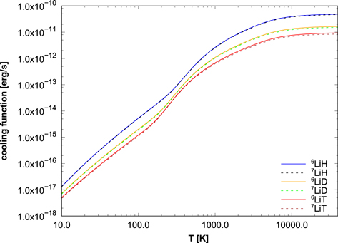
Figure 2. LiH radiative cooling functions for all isotopologues.
Download figure:
Standard image High-resolution image
Figure 3. 7LiH radiative cooling function for low temperatures.
Download figure:
Standard image High-resolution image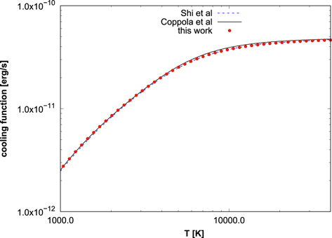
Figure 4. 7LiH radiative cooling function for high temperatures.
Download figure:
Standard image High-resolution imageTable 8. Radiative Cooling Function Fits for LiH Isotopologues
| Isotopologue | Coefficients | Isotopologue | Coefficients | Isotopologue | Coefficients |
|---|---|---|---|---|---|
| 7LiH | a0 = −32.0721 | 7LiD | a0 = −37.2617 | 7LiT | a0 = −38.5867 |
| a1 = 34.8115 | a1 = 50.4009 | a1 = 54.825 | |||
| a2 = −31.5332 | a2 = −50.4818 | a2 = −56.6013 | |||
| a3 = 15.1598 | a3 = 26.4059 | a3 = 30.3862 | |||
| a4 = −3.77326 | a4 = −7.25581 | a4 = −8.5735 | |||
| a5 = 0.460808 | a5 = 1.00031 | a5 = 1.2149 | |||
| a6 = −0.0217801 | a6 = −0.0547776 | a6 = −0.0684165 | |||
| 6LiH | a0 = −31.8095 | 6LiD | a0 = −37.0549 | 6LiT | a0 = −38.4451 |
| a1 = 34.0551 | a1 = 49.7459 | a1 = 54.3077 | |||
| a2 = −30.6588 | a2 = −49.6288 | a2 = −55.8166 | |||
| a3 = 14.6604 | a3 = 25.875 | a3 = 29.8476 | |||
| a4 = −3.62303 | a4 = −7.08599 | a4 = −8.38899 | |||
| a5 = 0.438038 | a5 = 0.973418 | a5 = 1.18415 | |||
| a6 = −0.0204103 | a6 = −0.0531076 | a6 = −0.0664301 |
Download table as: ASCIITypeset image
Comparing our curve with those of Coppola et al. and Shi et al. we see that it converges with the former at small T and with the latter at large T. As discussed in the previous section, while Shi et al. use a supposedly better empirical PEC, Coppola et al. use a better DMC. For the LTE radiative cooling function, the accuracy of the DMC is more relevant at lower temperatures, while the accuracy of the energy levels is dominant at higher temperatures. Hence, our curve corrects the physical behavior of the Shi et al. curve at low temperatures. Due to the very accurate potential energy and DMCs used here, we believe that our LTE cooling function is the most accurate one reported so far. It is interesting to note that although the choice made for the vibrational mass affects the transition energies, it is not relevant for the cooling function. The likely reason for this is that the largest Einstein coefficients are found for transitions between neighboring vibrational states, the only allowed transitions in the harmonic oscillator approximation, which are less sensitive to mass effects since the non-adiabatic corrections of neighboring vibrational states are of similar size.
Returning now to Figure 2, it can be seen that the LTE curves are grouped in pairs, 6LiX and 7LiX, with X = H, D, or T, the lighter isotopologues being better coolants than the heavier ones. The differences between the LTE cooling functions can be relevant for cosmological theory, except perhaps for the tritium-containing isotopologues, which are included here for completeness, since T would be much less abundant.
The behavior of the cooling functions with respect to the reduced mass can be rationalized as follows: within the harmonic oscillator-rigid rotor approximation, the energy of a diatomic molecule is given as

where B = ℏ2/(2I) is the rotational constant, and I = μR2 the moment of inertia. Since  , where κ is the force constant, we have
  and Erot ∝ 1/μ. The transition energies, ΔE, can be written as

for the R-branch, and

for the P-branch. The constants C1 and C2 scale with the reduced mass as  and C2 ∝ 1/μ.
Comparing the isotopologues of LiH, the one with the largest reduced mass has the closer energy levels, and thus the partition function, which yields the number of occupied states at a given temperature, is expected to be larger. The highest function is the one for 7LiT, and the lowest is the one for 6LiH. The reduced masses of the six isotopologues are collected in Table 9. As they are different, we expect six distinct curves in the plot of the partition functions in Figure 5. The small change in the reduced mass when 6Li is replaced by 7Li, of the order of 0.02–0.1 mp, explains that the six curves are separated into three pairs. In the LTE limit, the cooling functions are given by Equation (4). Figure 2 shows these functions for the six isotopologues. The presence of the partition function in the denominator of Equation (4), with its particular dependence on the reduced mass, leads to an inversion of the order of the six curves compared to Figure 5.

Figure 5. Partition functions for the six isotopologues.
Download figure:
Standard image High-resolution image
Table 9. Approximate Values of the Reduced Masses of Lithium Hydride Isotopologues in Units of the Proton Mass, mp
| Isotopologue | μ (mp) |
|---|---|
| 6LiH | 6/7 = 0.86 |
| 7LiH | 7/8 = 0.88 |
| 6LiD | 12/8 = 1.50 |
| 7LiD | 14/9 = 1.56 |
| 6LiT | 18/9 = 2.00 |
| 7LiT | 21/10 = 2.10 |
Download table as: ASCIITypeset image
The plot of the cooling functions also shows an interesting effect. At around T = 400 K the six curves approach each other considerably. A similar behavior has been obtained for HeH+ (Coppola et al. 2011), but no explication was given. This interesting effect can be understood in the following way. The DMC for LiH has a maximum at around Rmax = 5 a0, whereas the equilibrium distance in the vibrational ground state is about R0 = 3 a0; see Figure 1 of Diniz et al. (2016). The Einstein coefficients in Equation (2) assume particularly large values of the expectation values of the internuclear distance,  , if the two states are close to the maximum of the DMC. As augmentation of the reduced mass diminishes the expectation value
  , we conclude that for the lowest vibrational states, with
  , the isotopologues with larger reduced mass have smaller transition dipole moments and hence smaller Einstein coefficients, Aν'J'ν''J''. This, together with the mass-dependence of the partition function in the denominator of Equation (4), contributes to the separation of the six cooling functions. If, on the other hand, with increasing temperature, states having
  get considerably populated, the effect is inverted. Now, the isotopologues with larger reduced mass, and smaller
  , will have larger Einstein coefficients, which leads to an approximation of the six curves. In conclusion, while the partition functions govern the separation and order of the six curves, the behavior of the Einstein coefficients leads to an approximation of the six cooling functions within a certain temperature interval. Figure 5 shows that this approximation happens at around T = 400 K for the LiH isotopologues.
The following 72 tables are supplied as supplemental material: rovibrational energy values, P-branch data, R-branch data, LTE cooling function, for each of the six isotopologues and for the three choices of masses: nuclear, atomic, and effective. The most accurate values are those computed with effective masses, but we supply results obtained with constant masses for reference. Extracts from the full material can be found in Tables 10–13, where we display the first 10 lines for the 7LiH isotopologue and effective masses.
6. Conclusions
Whether LiH plays a role in the cooling of the primordial universe or not is still under discussion. In recent observations, a considerable abundance of LiH could not be detected in the Milky Way (Neufeld et al. 2017). However, the arguments related to its large dipole moment seem convincing enough to keep the idea alive. In order for theoretical models to be reliable, very accurate linelists, transition energies, as well as cooling functions, must be available. The possibility of heavier isotopologues being involved, mainly LiD, has never been considered. Rather than changing considerably the role of the dipole moment (as in the HD case), LiH isotopologues present large changes both in the number of rovibrational states, and in consequence, the possible transition energies, through reduced mass effects. The lighter isotopologues, 7LiH and 6LiH, are found to be the best prospective coolants. For a range of low temperatures around 400 K, however, the cooling functions approach each other. This feature seems to be connected to the behavior of the dipole moment with the nuclear distance, and has appeared in calculations for HeH+ and HeD+, despite apparently having gone unnoticed (Coppola et al. 2011). As we produce benchmark linelists taking into account relativistic, adiabatic, and non-adiabatic corrections for all stable isotopologues of LiH, we expect our data to be useful for astrophysicists in many other aspects.
J.R.M. acknowledges the CNRS for an invited scientist position at the University of Reims Champagne-Ardenne. A.A. thanks the Federal University of Minas Gerais (UFMG) and the French Embassy for awarding a Franco-Brazilian Chair at the UFMG. Support from the Brazilian agencies CNPq and FAPEMG is also acknowledged.
Appendix: Tables Supplied as Supplemental Material
72 tables are supplied, containing data for 6 isotopologues calculated with three choices of masses. These data are provided in plain format.
Example data for the 7LiH isotopologue and effective mass (rovibrational energy values, P-branch data, R-branch data and LTE cooling function) are shown in Tables 10–13.
Table 10. Rovibrational Energy Values for 7LiH Computed with Effective Masses
| v | J | State Energy |
|---|---|---|

|
||
| 0 | 0 | 0.000000 |
| 1 | 0 | 1359.684130 |
| 2 | 0 | 2674.501607 |
| 3 | 0 | 3945.391302 |
| 4 | 0 | 5173.185086 |
| 5 | 0 | 6358.632493 |
| 6 | 0 | 7502.365971 |
| 7 | 0 | 8604.930354 |
| 8 | 0 | 9666.715552 |
| 9 | 0 | 10687.908894 |
Note. The zero-point energy is −8.06714689 Eh.
Download table as: ASCIITypeset image
Table 11. P-branch Data for 7LiH Computed with Effective Masses
| A-coefficient | Transition Energy | v' | J' | v'' | J'' | Lower State Energy |
|---|---|---|---|---|---|---|
| (s−1) | ( ) ) |
( ) ) |
||||
| 4.683210E+01 | 1344.862070 | 1 | 0 | 0 | 1 | 14.822060 |
| 2.075757E+00 | 2659.679547 | 2 | 0 | 0 | 1 | 14.822060 |
| 8.571055E+01 | 1300.420410 | 2 | 0 | 1 | 1 | 1374.081197 |
| 9.495442E–03 | 3930.569242 | 3 | 0 | 0 | 1 | 14.822060 |
| 6.494893E+00 | 2571.310105 | 3 | 0 | 1 | 1 | 1374.081197 |
| 1.166234E+02 | 1256.910000 | 3 | 0 | 2 | 1 | 2688.481302 |
| 2.232554E–03 | 5158.363026 | 4 | 0 | 0 | 1 | 14.822060 |
| 5.480532E–02 | 3799.103889 | 4 | 0 | 1 | 1 | 1374.081197 |
| 1.348348E+01 | 2484.703784 | 4 | 0 | 2 | 1 | 2688.481302 |
| 1.396981E+02 | 1214.224487 | 4 | 0 | 3 | 1 | 3958.960599 |
Download table as: ASCIITypeset image
Table 12. R-Branch Data for 7LiH Computed with Effective Masses
| A-coefficient | Transition Energy | v' | J' | v'' | J'' | Lower State Energy |
|---|---|---|---|---|---|---|
| (s−1) | ( ) ) |
( ) ) |
||||
| 1.178221E–02 | 14.822060 | 0 | 1 | 0 | 0 | 0.000000 |
| 1.425954E+01 | 1374.081197 | 1 | 1 | 0 | 0 | 0.000000 |
| 1.120048E–02 | 14.397067 | 1 | 1 | 1 | 0 | 1359.684130 |
| 6.216878E–01 | 2688.481302 | 2 | 1 | 0 | 0 | 0.000000 |
| 2.607484E+01 | 1328.797172 | 2 | 1 | 1 | 0 | 1359.684130 |
| 1.062932E–02 | 13.979695 | 2 | 1 | 2 | 0 | 2674.501607 |
| 1.542250E–03 | 3958.960599 | 3 | 1 | 0 | 0 | 0.000000 |
| 1.963972E+00 | 2599.276469 | 3 | 1 | 1 | 0 | 1359.684130 |
| 3.542607E+01 | 1284.458993 | 3 | 1 | 2 | 0 | 2674.501607 |
| 1.006618E–02 | 13.569298 | 3 | 1 | 3 | 0 | 3945.391302 |
Download table as: ASCIITypeset image
Table 13. LTE Cooling Function for 7LiH Computed with Effective Masses
| Temperature | Partition | LTE Cooling Function |
|---|---|---|
| (K) | Function | (erg s−1) |
| 1.0000000E+01 | 1.3639685E+00 | 1.3164509E–17 |
| 1.0864772E+01 | 1.4353296E+00 | 1.6752767E–17 |
| 1.1804326E+01 | 1.5149696E+00 | 2.1346028E–17 |
| 1.2825131E+01 | 1.6033097E+00 | 2.7205702E–17 |
| 1.3934212E+01 | 1.7008430E+00 | 3.4639862E–17 |
| 1.5139203E+01 | 1.8081446E+00 | 4.4014236E–17 |
| 1.6448399E+01 | 1.9258766E+00 | 5.5768107E–17 |
| 1.7870810E+01 | 2.0547912E+00 | 7.0434269E–17 |
| 1.9416225E+01 | 2.1957324E+00 | 8.8662143E–17 |
| 2.1095285E+01 | 2.3496388E+00 | 1.1124381E–16 |
Note. Just as in Coppola et al. (2011), the tabulated temperatures range from 10 to 40,000 K, with temperature increments as in Exomol, i.e., Tn = 1.086477 × Tn–1, which yields 101 entries.
Download table as: ASCIITypeset image