


Abstract
There have been several attempts in the past to understand the nature of the collision of individual cases of interacting coronal mass ejections (CMEs). We selected eight cases of interacting CMEs and estimated their propagation and expansion speeds, and direction of impact and masses, by exploiting coronagraphic and heliospheric imaging observations. Using these estimates while ignoring the errors therein, we find that the nature of collisions is perfectly inelastic for two cases (i.e., 2012 March and November), inelastic for two cases (i.e., 2012 June and 2011 August), elastic for one case (i.e., 2013 October), and super-elastic for three cases (i.e., 2011 February, 2010 May, and 2012 September). Including the large uncertainties in the estimated directions, angular widths, and pre-collision speeds, the probability of a perfectly inelastic collision for the 2012 March and November cases drops from 98% to 60% and 100% to 40%, respectively, increasing the probability for other types of collision. Similarly, the probability of an inelastic collision drops from 95% to 50% for the 2012 June case, 85% to 50% for the 2011 August case, and 75% to 15% for the 2013 October case. We note that the probability of a super-elastic collision for the 2011 February, 2010 May, and 2012 September CMEs drops from 90% to 75%, 60% to 45%, and 90% to 50%, respectively. Although the sample size is small, we find good dependence of the nature of collision on the CME parameters. The crucial pre-collision parameters of the CMEs responsible for increasing the probability of a super-elastic collision are, in descending order of priority, their lower approaching speed, expansion speed of the following CME higher than the preceding one, and a longer duration of the collision phase.
Export citation and abstract BibTeX RIS
1. Introduction
Coronal mass ejections (CMEs) are episodic expulsions of magnetized plasma from the Sun into the heliosphere; they were discovered in the 1970s (Hansen et al. 1971; Tousey 1973). They are drivers of major space weather events that pose dangers to space- and ground-based technology. The different parts of a CME (i.e., sheath, shock, and cloud) have different effects on the Earth's magnetosphere (Tsurutani et al. 1988; Gonzalez et al. 1994; Echer et al. 2008). In the last few decades, significant progress has been made in understanding CMEs, including their morphological and kinematic evolution in the heliosphere, using observations from a series of imaging instruments located in space and on the ground combined with modeling efforts (Lindsay et al. 1999; St. Cyr et al. 2000; Zhao et al. 2002; Xie et al. 2004; Yashiro et al. 2004; Schwenn et al. 2005; Schwenn 2006; Vršnak et al. 2010; Chen 2011; Webb & Howard 2012). It is still impossible, however, to forecast when a CME will be launched from the Sun and difficult to forecast accurately its arrival time at a particular location in the heliosphere. Thus, accurate space weather forecasting remains a difficult task (Hess & Zhang 2015; Möstl et al. 2015; Tucker-Hood et al. 2015). Prior to having a facility such as the twin Solar TErrestrial RElations Observatory (STEREO) spacecraft (Kaiser et al. 2008), which allows continuous imaging of the vast distance between the Sun and Earth, CMEs were termed ICMEs (interplanetary CMEs) when detected away from the Sun, i.e., at 1 au, using in situ instruments. Various studies have identified signatures of CMEs in in situ observations based on their magnetic field, velocity, temperature, density, plasma composition, plasma wave, suprathermal particles, etc. (Borrini et al. 1982; Klein & Burlaga 1982; Gosling et al. 1987; Gloeckler et al. 1999; Lepri et al. 2001; Cane & Richardson 2003; Zurbuchen & Richardson 2006; Richardson & Cane 2010). However, if CMEs interact or collide with any other large-scale solar wind structures, their in situ signatures are modified and found to be different from the signatures of a typical individual CME. The interacting CME structures are classified as compound streams or multiple ejecta (Burlaga et al. 1987, 2002; Wang et al. 2002).
The possibility of CME–CME interactions was pointed out by Intriligator (1976) using in situ solar wind observations from the Pioneer 9 and 10 spacecraft. A typical individual CME passes over the Earth in around 20 hr while some structures take around several days and are possibly formed out of multiple CMEs (Marubashi & Lepping 2007; Dasso et al. 2009). The resulting complex structure from multiple CMEs may deposit its energy into the Earth's magnetosphere over a long duration and lead to intense geomagnetic storms (Wang et al. 2003; Farrugia & Berdichevsky 2004; Farrugia et al. 2006; Lugaz & Farrugia 2014). CME–CME interaction has been studied for more than a decade since Gopalswamy et al. (2001), using the Large Angle and Spectrometric Coronagraph (LASCO; Brueckner et al. 1995) on board the SOlar and Heliospheric Observatory (SOHO), provided the first observational evidence for it. Magnetohydrodynamics (MHD) numerical simulations have attempted to address the physical mechanism in CME–CME interactions and CME–CME-driven shock interactions, and their consequences (Vandas et al. 1997; Gonzalez-Esparza et al. 2004; Vandas & Odstrcil 2004; Lugaz et al. 2005, 2013; Wang et al. 2005; Xiong et al. 2006, 2007, 2009; Shen et al. 2013, 2014, 2016; Niembro et al. 2015). Realizing the importance of studying CME–CME interactions and the availability of wide-angle imaging observations of Heliospheric Imagers (HIs) with Coronagraphs (CORs) on board SECCHI/STEREO, almost a dozen cases of interacting CMEs have been reported in the literature in the last five years (e.g., Harrison et al. 2012; Liu et al. 2012; Lugaz et al. 2012; Martínez Oliveros et al. 2012; Möstl et al. 2012; Shen et al. 2012; Temmer et al. 2012; Webb et al. 2013; Ding et al. 2014; Lugaz & Farrugia 2014; Mishra & Srivastava 2014; Colaninno & Vourlidas 2015; Mishra et al. 2015a). These studies, based on simulations and observations, have discussed the evolution of CME-driven shocks, the resulting structures, the nature of CME–CME collisions, particle acceleration, as well as geoeffectiveness. Precise information about the nature of CME–CME collisions may help in determining the change between their pre- and post-collision dynamics. The use of post-collision dynamics is expected to give more accurate arrival times of CMEs at the Earth than the use of pre-collision dynamics (Mishra et al. 2015a).
Earlier studies on different candidates of interacting CMEs, using the mass and kinematics estimates from multiple-viewpoint observations of STEREO, have posed the question as to what determines the nature of collision varying from super-elastic (Shen et al. 2012, 2013, 2016; Colaninno & Vourlidas 2015) to inelastic (Lugaz et al. 2012; Temmer et al. 2012; Mishra & Srivastava 2014; Mishra et al. 2015a, 2015b). There were several limitations in some of these studies, such as the lack of consideration of oblique collision scenarios in three dimensions (3D), expansion speeds, and angular widths of the CMEs. These limitations and uncertainties were only addressed in detail by Shen et al. (2012) and Mishra et al. (2016). Although Shen et al. (2012) is a milestone in our understanding of the nature of CME–CME collisions, their study does not attempt to constrain the conservation of momentum to remain valid for the collision scenario as in Mishra et al. (2016), who included errors in the observed characteristics of the CMEs.
This present study is the next step after Mishra et al. (2016) in understanding the nature of collision of CMEs by analyzing several cases of colliding CMEs. Similar to the study of Mishra et al. (2016), we look at the role of CME characteristics, i.e., propagation direction, propagation speed, expansion speed, and angular size, in determining the nature of collision of CMEs. We attempt to find the uncertainties involved while assessing the nature of collision of CMEs by estimating the value of the coefficient of restitution (Newton 1687). We determine the CME characteristics using STEREO and SOHO observations and assess how a reasonable uncertainty in the measured characteristics changes the probability for one nature of collision to another. Section 2 describes the selection of CME events, their tracking in the heliosphere using available imaging observations, and estimates of their characteristics (i.e., kinematics and mass) in the pre- and post-collision phases. The analyses for the coefficient of restitution (e) for the selected cases and their interpretations are given in Section 3. The results from all of the cases are summarized in Section 4. The limitations of the present study are discussed in Section 5, and the conclusions are presented in Section 6.
2. Selection of Events
We first selected all pairs of CMEs launched in quick succession from almost the same source region on the Sun in the STEREO era up to the year 2013 which were identified as front-side halos or partial halos in SOHO/LASCO images. The CMEs of the STEREO era were chosen since their 3D parameters could be estimated. Further, we chose only those cases where the following CME had a larger speed than the preceding CME, and collision was expected beyond a couple of solar radii from the Sun. The role of magnetic forces not considered in present study are important close to the Sun; therefore, the cases likely to have collision close to the Sun are not included. Finally, we selected only those cases of interacting CMEs that could be clearly tracked in the heliosphere by at least one HI on board STEREO. Following these, in the present study, a total of eight cases of interacting CMEs that collided with one another before reaching the Earth are selected. Although the selected cases are still limited in number, we think that it may be extremely lengthy and difficult to select enough collision cases to perform a statistically significant study.
The selected CMEs could be tracked from the corona to the collision sites or beyond using the imaging instruments on board the STEREO spacecraft. The details of these selected cases of colliding CMEs are listed in Table 1. These eight events are classified into three categories based on three criteria: (i) availability of their observations from multiple viewpoints, (ii) distance of the collision sites from the Sun, and (iii) feasibility of marking the complete phase of collision duration. The duration of "collision" refers to the time interval during which exchange of momentum between the CMEs takes place as described in our earlier studies (Mishra et al. 2015a, 2016). The estimates for the observed collision duration of CMEs are not always precise. This is due to the poorly identified boundary of the collision directly from the observations. The errors in identifying the start and end of the collision lead to the errors in the measured pre- and post-collision dynamics of the CMEs. For two cases of colliding CMEs selected in our study, the end of the collision phase could not be identified. This compromises the accuracy of the estimated post-collision dynamics of such CMEs. The 3D kinematics of a CME can be estimated using only single viewpoint observations of HIs (Kahler & Webb 2007; Lugaz et al. 2009; Davies et al. 2012). This is because HIs image a CME at and across a large distance from the Sun where geometrical and Thomson scattering linearities break down (Howard 2011). However, earlier studies have shown that stereoscopic reconstruction methods applied to HI observations from multiple viewpoints of STEREO are more accurate than single-spacecraft reconstruction methods for the estimation of the kinematics of CMEs (Liu et al. 2010a; Lugaz et al. 2010; Davies et al. 2013; Mishra & Srivastava 2013; Mishra et al. 2014). Three of the selected events in our study were not well observed from both viewpoints of STEREO/HI, and therefore, we have to use single-spacecraft reconstruction methods for those cases. The accuracy of the kinematics estimated using only the single viewpoint observations would be limited. We point out that the CMEs colliding far from the Sun have large errors in their tracking and reconstruction, causing large uncertainties in their estimated kinematics (Liu et al. 2010b; Wood et al. 2010; Davies et al. 2012; Mishra et al. 2014, 2015b). The kinematics with limited accuracy will tend to reduce the accuracy of the analysis for those CMEs. Thus, the accuracy of our analysis will be highest for the cases where the three aforementioned criteria are met favorably by the CMEs, i.e., heliospheric observations from both HI-A and B are available, the collision site was not too far away from the Sun, and the collision phases could be clearly distinguished.
Table 1. Selected CME Events
| Events | STEREO Observations | Collision Sites | Collision Phase | Accuracy |
|---|---|---|---|---|
| 2011 Feb 14–15 | Both A and B | 24 
|
Well identified | Highest |
| 2012 Jun 13–14 | Both A and B | 100 
|
Well identified | Highest |
| 2010 May 23–24 | Both A and B | 42 
|
End phase poorly identified | Moderate |
| 2012 Mar 4–5 | Both A and B | 160 
|
Well identified | Moderate |
| 2012 Nov 9–10 | Only A | 30 
|
Well identified | Moderate |
| 2013 Oct 25 | Only B | 37 
|
Well identified | Moderate |
| 2011 Aug 3–4 | Both A& B | 145 
|
End phase not identified | Lowest |
| 2012 Sep 25–28 | Only A | 170 
|
Well identified | Lowest |
Note. From left: the first, second, third, fourth and fifth columns show the date of events, availability of observations from the STEREO spacecraft, distance of collision site from the Sun, feasibility of marking the boundaries of the collision phase, and accuracy assigned for the analysis, respectively. The estimate of the collision site is made from the derived kinematics of the colliding CMEs as described in Sections 2.1.1–2.1.8.
Download table as: ASCIITypeset image
Table 1 shows that all three criteria are met favorably for the cases of the 2011 February 14–15 and 2012 June 13–14 CMEs. Thus, these two cases have the highest accuracy in our analysis. The cases of the 2010 May 23–24, 2012 March 4–5, 2012 November 9–10, and 2013 October 25 CMEs favorably met only two criteria. Therefore, the analysis for these four cases is considered with moderate accuracy. The colliding CMEs of 2011 August 3–4 and 2012 September 25–28 only satisfy the criteria favorably and are noted to have the lowest accuracy among the cases selected for our study.
2.1. Tracking of the CMEs and Estimation of Their Kinematics in the COR and HI Fields of View
In this section, we track the CMEs in the heliosphere using the observations of STEREO coronagraphs (CORs) and HIs. To estimate the initial 3D kinematics of the CMEs, we reconstruct them in the COR field of view by applying the Graduated Cylindrical Shell (GCS) forward-fitting model (Thernisien et al. 2009) to the images obtained from STEREO/COR and SOHO/LASCO. We have attempted to fit the diffuse front of the CMEs, which seems to envelop the loop front. The diffuse front is often formed due to local density compression at a wave front while the loop front is formed due to transported piled-up plasma at the outer boundary of the flux rope. We note that the most difficult and important part in fitting halo CMEs is not fitting the two STEREO views but fitting the LASCO view. Further, the evolution of the CMEs is examined in the heliosphere by carefully examining the sequence of running and base-difference HI images. It is noted that the CME signals are not sufficient to track the specific features in the sequences of images. Therefore, we constructed the time-elongation maps, conventionally called J-maps, (Sheeley et al. 2008; Davies et al. 2009) using the running difference images of HI1 and HI2. The tracking and measuring of the time-elongation profiles of the evolving CMEs are carried out from the J-maps. Thereafter, an appropriate reconstruction method is applied on time-elongation profiles to estimate the 3D kinematics of the CMEs, which will be further used to identify the collision site, duration of collision, as well as pre- and post-collision dynamics. In light of the earlier studies regarding the relative performance of reconstruction methods (Lugaz 2010; Liu et al. 2013; Mishra et al. 2014), we use the stereoscopic self-similar expansion (SSSE; Davies et al. 2013) or self-similar expansion (SSE; Davies et al. 2012) method to the J-maps of the CMEs. The SSSE method is used for the CMEs observed in the HI field of view of both STEREO-A and B; otherwise, the SSE method is used when the CMEs were observed in either HI-A or HI-B only.
To implement either the SSE or SSSE methods, an input of the appropriate value of the cross-sectional angular half-width (λ) of the CME is required. For the SSE method, an additional input of the propagation direction of the CME is required. These inputs are obtained by applying the GCS model to the CMEs in the COR field of view. It has been highlighted that using different values of λ with the SSE or SSSE methods gives different estimates of the kinematics of the CMEs propagating away from the observer (Liu et al. 2013; Mishra & Srivastava 2015). Earlier studies have found that for CMEs propagating toward the Earth with STEREO behind the Sun, the SSE or SSSE method should be implemented with a λ value of 90° (Liu et al. 2013, 2014; Mishra et al. 2015b; Vemareddy & Mishra 2015). The error in the kinematics from the methods applied and the difference in the estimated direction of the CMEs in the COR and HI fields of view will be discussed in Section 5. In the following sections, we will describe the tracking, pre- and post-collision kinematics, and mass of the selected CMEs. The description of the selected cases is arranged sequentially in our study, considering the date of the events in ascending order and their assigned accuracy in descending order as per Table 1.
2.1.1. 2011 February 14–15 CMEs
The CMEs that launched on 2011 February 14 (hereinafter CME1) and February 15 (hereinafter CME2) have been analyzed before, focusing on the kinematics, related Forbush decrease (Maričić et al. 2014), their interaction corresponding to different position angles (Temmer et al. 2014), their geometrical properties, and the coefficient of restitution for the head-on collision scenario (Mishra & Srivastava 2014). Our present study focuses on the nature of collision in the oblique collision scenario and the uncertainties involved therein. The parameters for CME1 and CME2 for the best visual GCS fitting (Figure 2 of Temmer et al. 2014) are listed in Table 2. The 3D speeds of CME1 and CME2 are noted to be 420 km s−1 and 580 km s−1, respectively. The kinematics of CME1 and CME2 suggest their possible collision at some location in the heliosphere.
Table 2. Parameters for the CMEs Derived from the GCS Model
| Events | ϕ (°) | θ (°) | α (°) | κ | γ (°) | hf ( ) ) |
 /2 (°) /2 (°) |
|---|---|---|---|---|---|---|---|
| Feb 14 at 18:24 UT (CME1) | 6 | 4 | 32 | 0.28 | −8 | 10 | 16 |
| Feb 15 at 02:24 UT (CME2) | −3 | −11 | 18 | 0.37 | 25 | 11 | 22 |
| Jun 13 at 13:25 UT (CME1) | −15 | −26 | 20 | 0.55 | −64 | 13.5 | 33 |
| Jun 14 at 14:12 UT (CME2) | −2 | −31 | 31 | 0.6 | −45 | 14.2 | 37 |
| May 23 at 18:30 UT (CME1) | 12 | 6 | 23 | 0.26 | −55 | 16.3 | 15 |
| May 24 at 14:06 UT (CME2) | 26 | −5 | 15 | 0.37 | 6 | 14.5 | 22 |
| Mar 4 at 11:00 UT (CME1) | −55 | 23 | 20 | 0.6 | −36 | 16.5 | 37 |
| Mar 5 at 04:00 UT CME2) | −40 | 41 | 21 | 0.7 | −44 | 10.7 | 44 |
| Nov 9 at 15:12 UT (CME1) | 2 | −14 | 19 | 0.52 | 9 | 9.6 | 31 |
| Nov 10 at 05:12 UT (CME2) | 6 | −25 | 12 | 0.19 | 9 | 8.2 | 11 |
| Oct 25 at 08:15 UT (CME1) | −70 | 3 | 30 | 0.39 | 90 | 11.5 | 23 |
| Oct 25 at 15:15 UT(CME2) | −65 | 3 | 65 | 0.59 | 90 | 12.5 | 36 |
| Aug 3 at 14:00 UT (CME1) | 14 | 14 | 20 | 0.5 | −74 | 13 | 30 |
| Aug 4 at 04:12 UT (CME2) | 19 | 16 | 45.5 | 0.47 | 77 | 13 | 28 |
| Sep 25 at 11:24 UT (CME1) | 19 | −11 | 21 | 0.34 | 6 | 15 | 20 |
| Sep 28 at 00:12 UT (CME2) | 25 | 13 | 68 | 0.52 | −75 | 13 | 31 |
Note. The columns from left to right show the time of first appearance of the selected CMEs (CME1 and CME2) in LASCO-C2, longitude (ϕ), latitude (θ), half-angle (α) of the conical leg of the CME, aspect ratio (κ), tilt angle (γ) around the axis of symmetry of the model, height (hf) of the leading front, and edge-on 3D angular half-width ( /2) of the CME derived from implementing the GCS method of 3D reconstruction. The latitudes and longitudes are given in the Stonyhurst coordinate system (Thompson 2006) in which the Earth is always at the longitude of zero. The edge-on angular half-width is determined using the formulation given in Thernisien et al. (2006) and Thernisien (2011). The uncertainty in the propagation direction and half-angle is around ±5°, in tilt angle it is around ±20°, in aspect ratio it is around ±0.10, and in distance it is almost ±1.0
  . The GCS fitting uncertainties lead to an error of ±50 km−1 in speed values. The uncertainties in the GCS parameters are noted from several independent attempts of applying GCS model to the CMEs.
Download table as: ASCIITypeset image
The evolution of these CMEs in J-maps and the kinematics derived by implementing the SSSE method (Davies et al. 2013) on the time−elongation profile are respectively shown in Figures 7 and 8 of Mishra & Srivastava (2014). Based on the description of the collision phase in Mishra & Srivastava (2014), we note that the collision began on 2011 February 15 at 08:25 UT and ended after 18 hr. However, there is difficulty in precisely marking the start and end of momentum exchange between the CMEs, which is discussed in Section 5. Due to the collision, CME1 accelerated from u1 = 300 km s−1 to v1 = 600 km s−1 and CME2 decelerated from u2 = 525 km s−1 to  km s−1. We estimate the true masses of both CMEs using COR2 images, following the method of Colaninno & Vourlidas (2009). The masses of CME1 and CME2 are estimated to be 5.4 × 10¹² kg and 4.8 × 10¹² kg, respectively. The leading edge of CME2 is around 24 R☉ and that of CME1 was around 26 R☉ at the beginning of the collision.
2.1.2. 2012 June 13–14 CMEs
The CMEs of 2012 June 13 (hereinafter CME1) and June 14 (hereinafter CME2) appear to propagate southward in the COR2 images of STEREO, and CME2 appears wider than CME1. We have applied the GCS forward-fitting model to the contemporaneous images of the CMEs obtained from the SECCHI/COR2-B, SOHO/LASCO-C3, and SECCHI/COR2-A coronagraphs. We find the propagation direction of CME1 along E15S26 at 13.5  . The propagation direction for the following CME2 was along E02S31 at 14.2
  . In addition to the propagation directions, GCS-derived parameters for the CMEs are listed in Table 2. Around 14
  , the 3D speed of CME1 is noted as 560 km s−1 and for CME2 it is 900 km s−1. The directions and speeds of the CMEs suggest that they possibly collide during the heliospheric evolution.
These CMEs were well observed in the HI-A and HI-B fields of view of STEREO. The base-difference HI images and the constructed J-maps revealing the kinematic evolution of these CMEs are shown in Figure 1. The base image used here is the minimum background created from a sequence of HI images. The tracked features come in close contact with each other and appear to merge around 25° elongation and can be tracked farther up to 35°. The kinematics obtained from implementing the SSSE method on the derived time−elongation profiles of these CMEs are shown in the right panels of Figure 1. The collision began on 2012 June 15 at 08:38 and continued for 7.2 hr. At the beginning of the collision, the leading edge of CME2 was at 100  and that of CME1 was at 105
  . During the collision, they traveled a distance of around 25
  before reaching approximately equal speeds. The collision led to an acceleration of the preceding CME1 from 590 km s−1 to 680 km s−1 and a deceleration of the following CME2 from 865 km s−1 to 680 km s−1. The masses of CME1 and CME2 are estimated to be 8.4 × 10¹² kg and 9.2 × 10¹² kg, respectively.
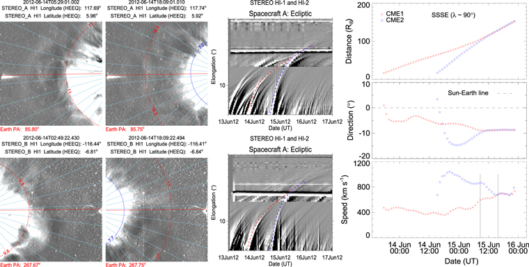
Figure 1. Left panel: in the top, the figures from left to right show the HI1-A base-difference images at two different times and the J-map constructed using the running difference images of HI1 and HI2. The bottom panel shows the same as the top but using HI-B images. The derived elongations of CME1 (with red) and CME2 (with blue) are overplotted on the HI images and J-maps. Right panel: from the top, the first, second, and third panels show the variation in distance, direction, and speed of the leading edge of the 2012 June CMEs. The vertical lines in the bottom panel mark the start and end of the collision phase.
Download figure:
Standard image High-resolution image2.1.3. 2010 May 23–24 CMEs
Analyses of the CMEs of 2010 May 23 (hereinafter CME1) and May 24 (hereinafter CME2) have been reported by Lugaz et al. (2012). The GCS-derived parameters (Figure 3 of Lugaz et al. 2012) of these CMEs are listed in the Table 2. The speeds of CME1 and CME2 at the outer edge of the COR field of view are estimated to be 450 km s−1 and 650 km s−1, respectively. Figure 4 and Figure 6 of Lugaz et al. (2012) show the J-maps constructed from the HI images and the derived kinematics for these CMEs, respectively. A big data gap from STEREO-B just after the beginning of the collision prevents the collision phase from being accurately marked; however, the data from STEREO-A serve our purpose with limited accuracy. It is noted that the leading edge of CME2 collided with the back of the magnetic ejecta of CME1 around 00:09 on May 25. Based on the analysis, we find that the collision duration is as short as 2.5 hr although large errors are expected (Lugaz et al. 2012). At the beginning of the collision, the leading edges of CME2 and CME1 were around 42  and 65
  from the Sun. The collision led to an acceleration of CME1 from 360 to 420 km s−1 and a deceleration of CME2 from 600 to 380 km s−1. The masses of CME1 and CME2 in the COR field of view, exploiting the multiple viewpoints of STEREO, are measured to be 4.5 × 10¹² kg and 2.2 × 10¹² kg, respectively.
2.1.4. 2012 March 4–5 CMEs
The GCS-derived parameters for the CMEs of 2012 March 4 (hereinafter CME1) and March 5 (hereinafter CME2) are shown in Table 2. The 3D speeds of CME1 and CME2 were around 1025 km s−1 and 1300 km s−1 at 16.5  and 10.7
  from the Sun, respectively. The base-difference HI images, constructed J-maps, and kinematic evolution of these CMEs are shown in Figure 2. The kinematics derived from the SSSE method show the collision signature as an exchange of momentum between CME1 and CME2. The commencement of collision is marked at 07:12 UT when the leading edge of CME2 was 160
  from the Sun and that of CME1 82
  from the Sun. The duration of the collision phase is around 4.8 hr. The exchange in dynamics of the participating CMEs in the collision is revealed as an increase in the speed of CME1 from 475 to 600 km s−1 and a decrease in the speed of CME2 from 910 to 700 km s−1. The masses of CME1 and CME2 are measured to be 4.6 × 10¹² kg and 13.5 × 10¹² kg, respectively. We emphasize that a relatively larger (≈
 ) difference in the latitudes of CME1 and CME2 (Table 2) does not perfectly represent a scenario of collision occurring in the ecliptic plane as assumed in our study. Our idealistic assumption would lead to estimated values for the propagation speeds, expansion speeds, and collision duration different from the values actually responsible for the physical nature of the collision. Such type of error is smaller for other selected cases of the CMEs.

Figure 2. Same as Figure 1, but for the 2012 March 4–5 CMEs.
Download figure:
Standard image High-resolution image2.1.5. 2012 November 9–10 CMEs
The estimated kinematics of the CMEs of 2012 November 9 (hereinafter CME1) and November 10 (hereinafter, CME2) in the COR and HI fields of view, using multiple-viewpoint observations of STEREO, have been reported by Mishra et al. (2015a). The obtained GCS-modeled parameters (Figure 2 of Mishra et al. 2015a) of these CMEs are tabulated in Table 2. From the kinematics, we note that CME2 is relatively narrow and directed more southward than CME1. The features of CME2 were not well observed in the STEREO-B ecliptic J-map, and the SSSE reconstruction technique could not be implemented to estimate the CME kinematics. Figures 4–6 in Mishra et al. (2015a) showed the constructed J-map, base-difference images of these CMEs with the elongation overplotted, and the kinematics obtained using the SSE method. The collision began at 11:30 UT on 2012 November 10 and lasted for 5.8 hr. The leading edges of CME2 and CME1 were at around 30  and 55
  from the Sun, respectively, at the commencement of the collision. The collision caused the speed of CME1 to increase from 365 to 450 km s−1 while causing the speed of CME2 to decrease from 625 to 430 km s−1. The masses of CME1 and CME2 were measured to be 4.7 × 10¹² kg and 2.3 × 10¹² kg, respectively, at the outer edge of the COR field of view.
2.1.6. 2013 October 25 CMEs
The two subsequently launched CMEs on 2013 October 25 are hereinafter referred to as CME1 and CME2, respectively. The GCS fitting parameters for these CMEs (Figure 1 of Mishra et al. 2016) are listed in Table 2. These CMEs were propagating eastward and largely away from the Sun−Earth line; therefore, their leading edge could not be observed in the HI-A field of view and only their flanks could be observed up to a small elongation angle. Therefore, we prefer to use only HI-B observations for our analysis. The constructed J-map and the derived time−elongation relation from this map overplotted on the HI-B images are shown in Figure 2 of Mishra et al. (2016), in which an obvious collision of the tracked features can be seen. The SSE method is implemented to estimate the CMEs' kinematics (Figure 3 of Mishra et al. 2016). We note that the collision began at 23:00 UT on 2013 October 25 and lasted for 7 hr. At the beginning of the collision, the leading edge of CME2 was around 37  from the Sun and that of CME1 at around 40
  from the Sun. The collision resulted in the exchange of dynamics, seen in the acceleration of CME1 from 425 to 625 km s−1 and in the deceleration of CME2 from 700 to 500 km s−1. The true masses of CME1 and CME2 are estimated to be 7.5 × 10¹² kg and 9.3 × 10¹² kg, respectively, in the STEREO/COR2 field of view.
2.1.7. 2011 August 3–4 CMEs
We list the GCS fitting parameters for the CMEs of 2011 August 3 (hereinafter CME1) and August 4 in Table 2. Around 13  , the speeds of CME1 and CME2 were 1100 km s−1 and 1700 km s−1, respectively, with their westward direction of propagation separated by only 5° from one another, ensuring a collision between them. Similar to the case studies discussed above, we construct the J-maps and then apply the SSSE method to determine the kinematics. The base-difference HI images, constructed J-maps, and the kinematics of these CMEs are shown in Figure 3. From the kinematics, we find that the collision began at 09:35 UT on 2011 August 5 when the leading edge of CME2 was at around 145
  and that of CME1 was at around 150
  from the Sun. Because of the extremely weak signal from the CMEs even in the J-maps, these CMEs could not be tracked longer, and therefore, the end phase of the collision could not be marked. The collision occurred near the Earth, and these CMEs were found to have equal speeds in in situ observations at 1 au. Thus, we consider the post-collision speeds of the CMEs as measured in situ at 1 au. The uncertainties arising from this will be discussed in Section 5. The collision led to an acceleration of CME1 from 420 to 525 km s−1 at the cost of decelerating CME2 from 630 to 525 km s−1. The true masses of CME1 and CME2 are determined to 7.4 × 10¹² kg and 10.2 × 10¹² kg, respectively.
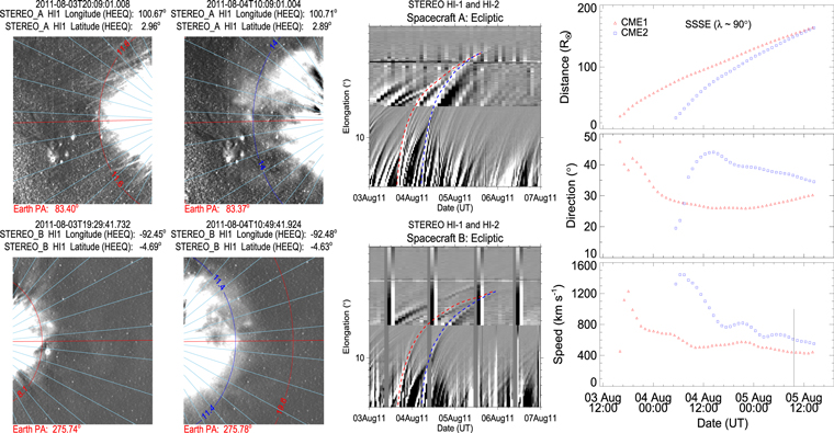
Figure 3. Same as for Figure 1, but for the 2011 August 3–4 CMEs.
Download figure:
Standard image High-resolution image2.1.8. 2012 September 25–28 CMEs
The CMEs of 2012 September 25 (hereinafter CME1) and September 28 (hereinafter CME2) have been analyzed in depth earlier, focusing on their interaction and the formation of a complex ejecta resulting in a two-step geomagnetic storm (Liu et al. 2014; Mishra et al. 2015b). Figure 1 of Mishra et al. (2015b) showed the GCS fitting wireframe on the CMEs, and the fitting parameters are listed in Table 2. The signals from these CMEs in the J-map constructed using HI-B images are too weak to track without ambiguity beyond 20°. Therefore, we could not implement the SSSE method. Instead, we used the SSE method with HI-A observations. We refer to Figures 3 and 6 of Mishra et al. (2015b) for the J-map and obtained the kinematics for these CMEs. We note that the collision led to an acceleration of CME1 from 385 to 710 km s−1 and a deceleration of CME2 from 610 to 430 km s−1. The collision phase began at 22:48 UT on 2012 September 29 and lasted for 16.8 hr. At the beginning of the collision, the leading edge of CME2 was around 170  and that of CME1 was around 190
  from the Sun. The true masses of CME1 and CME2 participating in the collision have also been estimated and found to be 1.8 × 10¹² kg and 9.7 × 10¹² kg, respectively.
3. Coefficient of Restitution of the CMEs: Analysis and Outcome
Knowledge of the coefficient of restitution (e) for colliding CMEs may be useful in accounting for some false CME arrival alarms and help predict their arrival at the Earth more accurately. In the present study, we treat CMEs as large expanding blobs and attempt to understand their bounciness for different cases. Using the expansion speeds of CME1 and CME2 (i.e.,  and
and  ) and their estimated leading edge speeds (i.e., u1 and u2) before the collision, we determined the speeds of their centroids (i.e., u1c and u2c) to use in studying the nature of collision. We assume that a CME expands in such a way that its angular width remains constant. It is difficult to know the true angular width of the CME approximated as a spherical bubble. The GCS model considers a CME to be a hollow croissant, which enables the face-on and edge-on angular widths to be estimated (Thernisien et al. 2009; Thernisien 2011). The edge-on angular width of a CME basically represents the width of the conical legs of the tubular front that makes up the GCS structure. The edge-on angular half-width is the inverse trigonometric sine function of the fitted aspect ratio (κ) of the CME from the GCS model. κ represents the rate of expansion versus the height of the CME, i.e., it is the ratio of the CME size at two orthogonal directions. Hence, the edge-on angular width best suits our purpose. The angular half-widths (ω) of the CMEs taken to be the edge-on angular half-width (ωEO/2) are listed in Table 2. We also determine the post-collision directions and speeds of the centroids of the CMEs. Further, we assumed no change in the angular widths of the CMEs before and after the collision.
We acknowledge the errors in the observed kinematics of the CMEs and the possibility of their deflection during the collision. The post-collision direction of the CMEs remains an observationally unknown parameter due to the interrelatedness of the post-collision dynamics and the nature of collision. Therefore, we determined the expected (i.e., theoretical) post-collision speeds of the centroids of the CMEs ( ) for a certain value of the coefficient of restitution (e) based on the momentum conservation law. The estimated expected post-collision speeds of the centroids are converted into their corresponding leading edge speeds (
 ), which will be compared with the observed leading edge speeds (
 ) of the CMEs by calculating the deviation (σ) between them. After several iterations, the best-suited e value of the collision of the CMEs is found at the minimum of the deviation (σ). It is noted that the value of e ranges between 0 and 5 during the iteration accounting for all possible natures of the collision. We also emphasize that a σ value of up to 150 km s−1 is satisfactory as this implies an average difference of only up to 100 km s−1 between the observed and expected speeds of the individual CMEs. Including the errors in tracking the CMEs and the 3D reconstruction and those raised from idealistic geometrical assumptions, an error of around ±100 km s−1 in the speed of the CMEs is not unexpected. The mathematical formulation applied in the present study is given in Mishra et al. (2016) with details; however, their core equations are also mentioned in Appendix
3.1. 2011 February 14–15 CMEs
The edge-on angular half-widths of CME1 and CME2 (i.e.,  and
and  ) are around 16° and 22°, respectively, as noted in Table 2. Considering no obvious deflection of the CMEs before the collision in the HI field of view, the estimated directions (i.e., ϕ) from the GCS model in the COR2 field of view (Table 2) are used for the pre-collision directions. Under the oblique collision scenario, using the estimated kinematics and angular widths of the CMEs in Equations (2) and (3) given in Appendix
Under the oblique collision scenario, we determined the direction of impact  ) for the collision. By direction of impact we mean the angle between the line connecting the centroids of two colliding CMEs and the propagation velocity of CME2 relative to CME1. We also determined several parameters of the CMEs just at the beginning of the collision together with other collision parameters. Using the expansion and propagation speeds estimated from the observations of the 2011 February 14–15 CMEs, we determined the ratio of the expansion speed (
 /
/ ) of CME2 to that of CME1, the sum of their expansion speeds (
 ), the pre-collision relative approaching speeds (
 ) of the centroids of the CMEs, and the post-collision relative separation speeds (
 ) of the centroids of the CMEs along the line joining their centroids. The details of the characteristics of the CMEs for the observed oblique collision are listed in Table 3. These parameters are also calculated for all cases selected in our study. We attempt to compare these parameters for all cases and examine whether they show a pattern for a particular nature of collision.
Table 3. CME Parameters under Oblique Collision
| Events | e (σ) (km s−1) | ΔKE, Δp1, Δp2 (%) | u1c, u2c |
 (km s−1) (km s−1) |
 / /
|
 (km s−1) (km s−1) |
 (km s−1) (km s−1) |
ψ (°) | ΔT (hr) | m2/m1 | R ( ) ) |
e1D ( ) (km s−1) ) (km s−1) |
|---|---|---|---|---|---|---|---|---|---|---|---|---|
| Feb 14–15 | 1.65 (120) | 7.3, 68, −43 | 235, 380 | 208 | 2.2 | 130 | 230 | 3.6 | 18 | 0.8 | 24 | 0.9 (142) |
| Jun 13–14 | 0.35 (40) | −1.7, 24, −15 | 380, 540 | 533 | 1.56 | 135 | 45 | 21.9 | 7.2 | 1.1 | 100 | 0 (77) |
| May 23–24 | 1.4 (15) | 1.8, 27, −30 | 285, 435 | 237 | 2.2 | 100 | 135 | 6.6 | 2.5 | 0.5 | 45 | 0.25 (43) |
| Mar 4–5 | 0 (20) | −3.5, 53, −9 | 295, 535 | 551 | 2.0 | 210 | −10 | 12.3 | 4.8 | 2.94 | 160 | 0 (224) |
| Nov 9–10 | 0 (25) | −13.4, 38, −36 | 240, 525 | 224 | 0.8 | 280 | −60 | 0.5 | 5.8 | 0.48 | 30 | 0.1 (9) |
| Oct 25 | 1.0 (50) | 0, 48, −26 | 305, 440 | 378 | 2.2 | 130 | 140 | 7.9 | 7.0 | 1.24 | 37 | 0.45 (20) |
| Aug 3–4 | 0.1 (40) | −3.7, 31, −15 | 280, 430 | 341 | 1.4 | 145 | −5.0 | 6.6 | obscure | 1.37 | 145 | 0 (24) |
| Sep 25–28 | 2.0 (30) | 3.34, 99, −13 | 285, 405 | 305 | 2.1 | 110 | 250 | 9.7 | 16.8 | 5.53 | 170 | 0.8 (120) |
Note. From left to the right: the first column shows the selected cases of colliding CMEs. The second and thirteenth columns list the estimated values of the coefficient of restitution (e) and deviation (σ) determined in the oblique and head-on collision scenarios, respectively. The third column lists the total change in the kinetic energy of the CMEs and the change in the momentum of CME1 and CME2. The fourth column shows the pre-collision centroid speeds (i.e., propagation speed) of CME1 and CME2. The fifth, sixth, and seventh columns show the sum of the expansion speeds of the colliding CMEs, the ratio of the CME2 to CME1 expansion speeds, and the relative approaching speeds of the centroids of the CMEs along the line joining their centroids, respectively, at the beginning of the collision. The eighth column shows the post-collision relative separation speed of the centroids of the CMEs along the line joining their centroids. The ninth, tenth, eleventh, and twelfth columns show the direction of impact, duration of collision phase, the ratio of the mass of CME2 to that of CME1, and the distance of the collision site from the Sun, respectively. The positive and negative signs show the increase and decrease in the parameters, respectively.
Download table as: ASCIITypeset image
In the following sections, we discuss the uncertainties in the propagation direction (ϕ), angular size (ω), and initial speed (u) of the CMEs, and their effects on the collision nature. We keep in mind that the collision condition should be satisfied while taking the uncertainties in the CME parameters. The condition requires that the speed of the leading edge of CME2 be greater than or equal to the speed of the trailing edge of CME1 along the line joining their centroids. In addition, the separation angle between the CMEs should be less than or equal to the sum of their angular half-widths (see Appendix
3.1.1. Effect of Propagation Direction
Including the errors in the estimated directions of the CMEs from the GCS model and the possibility of deflection of the CMEs with or without collision, the uncertainty in the estimated value of e, as mentioned in Table 3, is expected. We consider an arbitrary uncertainty of ±20° in the estimated longitudes of CME1 and CME2 (i.e.,  and
and  ). Using different pairs of longitudes, the estimated values of e and σ are shown in the top and bottom sections of the left panel of Figure 4. From this panel, it is clear that the nature of collision of these CMEs is super-elastic in nature. The values of e at the top-left and bottom-right panels correspond to two extreme values (i.e., 0 or 5) with large values of σ. These larger values of σ, which correspond to a larger separation angle between the CMEs, suggest lesser reliability of those e values. The larger values of σ imply that the expected dynamics of the CMEs satisfying momentum conservation do not represent the observed collision picture. The large σ value may be partly due to the errors in the propagation directions and observed speeds obtained along a different direction. The probability of a different nature of collision given the uncertainty in the propagation direction and corresponding range of deviation is given in Table 4.

Figure 4. From left: the first panel shows the variation of the coefficient of restitution (e) in the top panel and the corresponding deviation (σ) between the expected and observed pre-collision speeds in the bottom panel, for the uncertainties in the propagation direction of the 2011 February CMEs. The propagation directions of CME1 and CME2 ( and
and  ) are shown on the X- and Y-axes, respectively. The second and third panels show the variation of e and σ when the uncertainties in the angular width of the CMEs are considered. The angular half-widths of CME1 and CME2 (i.e.,
  and
and  ) are shown on the X- and Y-axes. The expansion speeds of CME1 and CME2 (i.e.,
  and
and  ) are shown on the top X-axis and the right-side Y-axis, respectively. The fourth panel shows the variation of e and σ when the uncertainties in the initial speed of the CMEs are considered. In the third and fourth panels, the X- and Y-axes, respectively, show the relative approaching speeds (
 ) and sum of the expansion speeds (
 ) of both CMEs. The color bars showing the range of values corresponding to each figure are stacked.
Download figure:
Standard image High-resolution imageTable 4. Effect of the ±20° Errors in the Observed Propagation Direction of the CMEs on the Nature of Their Collision
| Events | Probability for [e = 0, 0 < e < 1, e > 1, Δperr] (%) | σ for [e = 0, 0 < e < 1, e > 1, Δperr] (km s−1) | e for Δperr |
|---|---|---|---|
| Feb 14–15 | 0, 0.1, 87.7, 12.2 | NA, NA, 75–230, 235–255 | 0 |
| Jun 13–14 | 0, 65.1, 21.7, 13.2 | NA, 35–45, 25–100, 125–230 | 0 |
| May 23–24 | 0, 40.8, 39.5, 19.7 | NA, 5–115, 10–125, 140–160 | 0 |
| Mar 4–5 | 61.8, 23.7, 10.3, 4.2 | 1-45, 0–5, 5–175, 150–215 | 0 and 5 |
| Nov 9–10 | 48.3, 34.3, 16, 1.4 | 10–175, 1–15, 20–150, 160–175 | 0 |
| Oct 25 | 0, 15.1, 67.2, 8.9 | NA, 50–52, 25–165, 180–250 | 0 |
| Aug 3–4 | 0, 76.6, 18.8, 4.6 | NA, 30–40, 20–110, 115–170 | 0 |
| Sep 25–28 | 0, 0, 89.2, 10.8 | NA, NA, 30–290, 260–310 | 0 and 5 |
Note. The probability for the nature of collision due to an uncertainty of ±20° in the observed propagation direction (ϕ) of the CMEs. The first column shows the selected cases of colliding CMEs. The second and third columns, respectively, show the probability for the different natures of collisions (perfectly inelastic as e = 0, inelastic as 0 < e < 1, super-elastic as e > 1, and erroneous momentum exchange as Δperr) and the corresponding range of deviation (σ) values. Δperr stands for the scenario of an unexpected decrease in the momentum of CME1 and an increase in the momentum of CME2. The values of the coefficient of restitution (e) corresponding to the points of incorrect momentum exchange (Δperr) are noted in the fourth column.
Download table as: ASCIITypeset image
We also note that an increase in the error of the longitude from ±1° to ±20° causes a decrease in the probability of super-elastic collision from 100% to 87.7% with a mean deviation of around 120 km s−1. The increasing errors in the longitude increases the probability of perfectly inelastic (i.e., e = 0) collision from 0% to 12.2% with a large value of the mean deviation in speed of around 240 km s−1. We note that 12.2% of data points are unreliable, as they cause a decrease in the momentum of CME1 and an increase in the momentum of CME2 (i.e., for Δperr), thus apparently violating the momentum exchange condition (second column of Table 4). All these points violating the momentum exchange condition correspond to e = 0 (4th column of Table 4) and to a few of the maximum values of deviation in observed speed (third column of Table 4). We note that the uncertainty in the directions of the 2011 February 14–15 CMEs causes a modification in the value of e. This modification would be deceptive if the larger value of deviation (σ) in the speed is overlooked.
3.1.2. Effect of Angular Size
The angular size of the CME affects its expansion and centroid speeds when its leading edge speed is kept constant. Using the observed kinematics as noted in Section 2.1.1, we arbitrarily consider the angular width variation between 5° and 35° and repeat the calculation for e. The estimated values of e and σ are shown in the top and bottom of the second (from the left) panel of Figure 4. The findings of e, σ, range of  /
/ , and
, and  /
/ for a super-elastic and an inelastic collision, the percentage of data points for super-elastic collisions corresponding to the values of
  , and the percentage of data points among inelastic collisions with a larger sum of the expansion speeds than the relative approaching speeds of the CMEs are listed in Table 5. We note that even such a large uncertainty in the angular width results in a probability of 73.2% for a super-elastic collision, only 25.8% for an inelastic collision, and zero probability for a perfectly inelastic collision. The bottom-right corner shows
  and the corresponding deviation ranges from 80 to 140 km s−1. The deviation ranges between 10 and 175 km s−1 for the estimated super-elastic nature of collision. σ is large when the CME2 angular width, and hence its expansion speed, is larger than that of the observed value. The e values for super-elastic collision correspond to the ratio of the CME2 to CME1 expansion speeds between 0.6 and 7.9. This gives the ratio of the CME2 to CME1 angular widths ranging from 0.27 to 7. Among these values of e, around 96% have a larger expansion speed for CME2 than for CME1. However, e values for inelastic collision correspond to the ratio of the CME2 to CME1 expansion speeds ranging between 0.35 and 1.54, and to the ratio of the CME2 to CME1 angular widths ranging between 0.14 and 0.8. Among these values for inelastic collision, only around 47.5% have a larger expansion speed for CME2 than for CME1.
Table 5. Effect of the Errors on the Angular Size (5°–35°) of the CMEs on the Nature of Their Collision
| Events | Probability for [e = 0, 0 < e < 1, e > 1] (%) | σ for [e = 0, 0 < e < 1, e > 1] (km s−1) |
 / / ( ( / / ) for e > 1 ) for e > 1 |
 / / ( ( / / ) for 0 < e < 1 ) for 0 < e < 1 |
e > 1 among  > 1 (%) > 1 (%) |
e > 1 among  > 2 (%) > 2 (%) |
0 < e < 1 with  > 1 (%) > 1 (%) |
|---|---|---|---|---|---|---|---|
| Feb 14–15 | NA, 25.8, 73.2 | NA, 80–140, 10–175 | 0.60–7.9 (0.27–7) | 0.38–1.54 (0.14–0.8) | 84.7 | 100 | 39.5 |
| Jun 13–14 | 19.7, 50.4, 29.7 | 0–150, 0–70, 0–145 | 0.64–4.8 (0.38–4.2) | 0.44–2.0 (0.23–1.6) | 31.6 | 42.8 | 97.9 |
| May 23–24 | 1.0, 54.9, 43.6 | 155–160, 0–150, 0–160 | 0.56–7.6 (0.28–7) | 0.36–2.8 (0.14–1.8) | 48.9 | 64 | 78.7 |
| Mar 4–5 | 65, 26, 8.8 | 25–205, 25–125, 30–160 | 0.89–8.7 (0.4–7) | 0.74–5.6 (0.33–4.1) | 11.1 | 24.7 | 97.5 |
| Nov 9–10 | 40.7, 58, 1.3 | 0–50, 0–45, 25–30 | 5.6–7.8 (4.9–7.0) | 0.75–6.8 (0.38–5.6) | 2 | 5.8 | 78.4 |
| Oct 25 | 0.8, 74.9, 23.8 | 15–20, 0–55, 0–50 | 1.6–7.5 (1–7) | 0.39–2.7 (0.16–1.9) | 32.1 | 57.9 | 63.8 |
| Aug 3–4 | 37.3, 53.1, 9.4 | 0–65, 0–55, 10–55 | 2.8–6.8 (2.5–7) | 0.89–4.4 (0.56–3.6) | 11.8 | 21.2 | 92.1 |
| Sep 25–28 | 0, 39.1, 60.2 | NA, 40–85, 20–145 | 0.94–7.2 (0.56–7) | 0.35–1.44 (0.14–0.89) | 74.1 | 99.7 | 48.1 |
Note. The probability for the nature of collision due to a varying 3D edge-on angular half-width of the CMEs (i.e.,  and
and  ) between 5° and 35°. From left, the first, second, and third columns show the selected cases of colliding CMEs, the probability for the different natures of collisions, and the corresponding range of deviation (σ) values, respectively. The fourth (fifth) column shows the ratio of the expansion speed (angular widths) of CME2 to that of CME1 for the points having e > 1 and for the points with 0 < e < 1, respectively. The sixth (seventh) column shows the percentage of points having
  among the points that correspond to the sum of the expansion speeds (
 ) of CME1 and CME2 greater (two times greater) than the relative approaching speeds of the centroids (
 ) of the CMEs. The eighth column shows the percentage of data points with
  with the values of
  greater than the values of
  of the CMEs.
Download table as: ASCIITypeset image
As suggested in the earlier studies of Shen et al. (2012, 2016), we examined the characteristics of the collision using the relative approaching speed of the centroids of the CMEs along the line joining their centroids ( ) and the sum of their expansion speed (
 ) at the beginning of collision. The top and bottom of the third panel (from the left) of Figure 4 shows the variation in the e and σ values. From this panel, it is clear that there is no large value of σ for a particular type of collision. The nature of the collision tends to be super-elastic when the value of
  becomes larger than the values of
  . For instance, as quoted in Table 5, among the data points with values of
  larger than their values of
  , around 84.7% of the points show a super-elastic (e > 1) collision. Among the data points that have values of
  more than twice the value of
  , around all of the points (i.e., 100%) correspond to super-elastic collision. But for the data points corresponding to inelastic (0 < e < 1) collision, only 39.5% have values of
  larger than the values of
  . Thus, our finding is in agreement with that previously conceptualized in Shen et al. (2012, 2016).
3.1.3. Effect of Initial Speed
We consider an uncertainty of ±100 km s−1 in the observed pre-collision leading edge speed of the CMEs without changing their other observed parameters. We repeat the calculation as aforementioned, and the estimated values of the coefficient of restitution (e) and deviation (σ) are shown in the top and bottom of the fourth panel (from the left) of Figure 4. The estimated values of e, σ, range of  /
/ for super-elastic and inelastic collisions, the percentage of data points for super-elastic collisions corresponding to the values of
  , and the percentage of data points among inelastic collisions with the sum of the expansion speeds larger than the relative approaching speed of the CMEs are listed in Table 6. We note the probability of 2.4% for perfectly inelastic, 3.3% for inelastic (i.e.,
  1), and 88.8% for super-elastic collisions. The value of σ is not specifically large for a particular type of collision, and therefore, the estimated values of e are reliable. Among all of the data points corresponding to values of
  larger than their values of
  , around 96.8% show super-elastic collisions. However, there are no points with 0 < e < 1 having the sum of the expansion speeds larger than the relative approaching speeds.
Table 6. Effect of the ±100 km s−1 Errors in the Observed Speed of the CMEs on the Nature of Their Collision
| Events | Probability for [e = 0, 0 < e < 1, e > 1] (%) | σ for [e = 0, 0 < e < 1, e > 1] (km s−1) |
 / / for e > 1 for e > 1 |
 / / for 0 < e < 1 for 0 < e < 1 |
e > 1 among  > 1 (%) > 1 (%) |
0 < e < 1 with  > 1 (%) > 1 (%) |
|---|---|---|---|---|---|---|
| Feb 14–15 | 2.4, 3.3, 88.8 | 155–170, 110–130, 75–165 | 1.4–3.6 | 3.4–3.9 | 96.8 | 0 |
| Jun 13–14 | 0, 93.8, 6.2 | NA, 1–90, 30–65 | 1.2–1.3 | 1.2–2.0 | 6.2 | 100 |
| May 23–24 | 8.6, 25.2, 60.7 | 65–100, 0–40, 0–90 | 1.6–2.7 | 2.7–3.5 | 60.7 | 74.4 |
| Mar 4–5 | 97.9, 2.1, 0 | 15–65, 55–60, NA | NA | 1.8–1.9 | NA | 100 |
| Nov 9–10 | 100, 0, 0 | 15–75, NA, NA | NA | NA | NA | NA |
| Oct 25 | 0.4, 49.6, 49.2 | 102, 5–95, 10–95 | 1.5–2.1 | 2.2–3.2 | 49.2 | 100 |
| Aug 3–4 | 15.3, 84.3, 0.4 | 0–20, 10–90, 55 | 0.97 | 0.99–2.18 | 0.4 | 100 |
| Sep 25–28 | 0, 50.4, 48.8 | NA, 1–85, 2–95 | 1.5–2.1 | 2.2–3.3 | 48.7 | 100 |
Note. The probability for the nature of collision due to an uncertainty of ±100 km s−1 in the observed pre-collision speeds of the CMEs. The first to sixth columns are the same as in Table 5. The seventh column shows the same information as the eighth column in Table 5. The entry of "NA" in some parts of the table refers to "Not Applicable," and the value there has no meaning.
Download table as: ASCIITypeset image
We note that the ratio of the expansion speed of CME2 to that of CME1 ranges from 1.4 to 3.6 for  and 3.4 to 3.9 for
  . Thus, we do not notice that a large expansion speed of CME2 gives a higher probability of super-elastic collisions over inelastic ones. The values of e with a negative approaching speed are not reliable as it is related to a significantly larger value of the deviation. A negative approaching speed implies that the collision of the CMEs took place because of their larger expansion speed. From the analysis of the 2011 February CMEs, it is obvious that a decrease in the approaching speed increases the probability of a super-elastic collision. From the analysis, we found that even with the large uncertainties chosen in the directions, sizes, and speeds of the CMEs, the most probable nature of the collision for the CMEs of 2011 February is super-elastic.
3.2. 2012 June 13–14
The estimated coefficient of restitution (e) and the corresponding parameters for the CMEs of 2012 June 13–14 participating in the observed oblique collision scenario are listed in Table 3. The value of e is found to be 0.35 with a σ of 40 km s−1. However, in the head-on collision scenario, the value of e is noted as zero. The nature of collision is understood to be inelastic, which caused a decrease in the total kinetic energy of the CMEs of 1.7%, an increase in the momentum of CME1 of 24%, and a decrease in the momentum of CME2 of 15% compared to their values before the collision. The analysis for assessing the uncertainties in e is done in a similar manner that for the 2011 February 14–15 CMEs described in Section 3.1. The results obtained due to the uncertainties in the propagation directions, angular half-widths, and speeds are given in Tables 4–6, respectively, and shown in the Figure 5. Increasing the uncertainties in the propagation directions by up to ±20° leads to an increase in the probability of around 13.2% for a perfectly inelastic collision and around 21.7% for a super-elastic collision. The larger probability of around 65.1% for inelastic (0 < e < 1) collision has a value of σ between 35 and 45 km s−1 smaller than other types of collision. The data points for perfectly inelastic collision violate the momentum exchange condition and also give larger values of σ (i.e., 125–230 km s−1), and thus become unreliable.

Figure 5. Same as Figure 4, but for the 2012 June 13–14 CMEs. The white dashed lines mark the region of 0 < e < 1.
Download figure:
Standard image High-resolution imageTable 5 and the second panel from left in Figure 5 also give preference for the inelastic nature of collision. We note that the data points for super-elastic collisions give the ratio of the CME2 to CME1 expansion speeds (angular widths) ranging between 0.64 and 4.8 (0.38 and 4.2), which is larger than the ratio for the inelastic nature of collision. The third panel of the figure shows an increase in the probability of a super-elastic collision with a decrease in the relative approaching speed ( ). Among the points that have sums of the expansion speeds (u12exs) of the CMEs that are larger than their relative approaching speeds (u12cjr), there are around 31.6% points with e > 1. The probability of super-elastic collision increases with the increasing ratio of
  to
to  of the CMEs. For instance, among the points with values of
  five times larger than their values of
  , around 76% have e > 1. However, among all the points with 0 < e < 1, there are around 98% points that have larger values of u12exs than the values of u12cjr. There is zero probability of having values 0 < e < 1 among points with
  six times greater than
  . The uncertainty in the speed also gives a larger probability for inelastic collisions with typically smaller values of σ (fourth panel of Figure 5). However, no significant difference between the CME2 and CME1 expansion speeds is noted for super-elastic and inelastic collisions (Table 6). Among the points with values of
  larger than their
  values, 6% of the points have e > 1. Further, among the points with values of
  fifteen times larger than their values of
  , all of the points have e > 1. Carefully looking at the values noted in the second row of Tables 4–6, we decide that the nature of collision is inelastic for the CMEs of 2012 June 13–14.
3.3. 2010 May 23–24
Using the CME parameters observed in the oblique collision scenario, the value of e is 1.4 and the corresponding changes in the energy and momentum of the CMEs are listed in the third row of Table 3. The value of e in the head-on collision scenario is 0.25, which is largely underestimated. The effect of the uncertainties in the propagation directions, angular half-widths, and initial speeds on the collision characteristics is shown in Figure 6 and listed in the third row of Tables 4–6, respectively. The uncertainties in the propagation directions of up to ±20° lead to a decrease in the probability for super-elastic collision from 100% to 39.5%, and an increase in the probabilities for inelastic collision from 0% to 40.8% and for perfectly inelastic collision from 0% to 19.7%. Perfectly inelastic collision is not reliable as it violates the momentum condition and gives a large value of σ.

Figure 6. Same as Figure 4, but for the 2010 May 23–24 CMEs.
Download figure:
Standard image High-resolution imageTable 5 shows a larger probability for inelastic collision for these CMEs. From the table, we note that the ratios of the CME2 to CME1 expansion speeds ( /
/ ) and angular widths (
 /(
/( ) are significantly larger for e > 1 than for 0 < e < 1. Based on the number of data points, the probability of e > 1 increases from 48.9% to 92.1% as the ratio of
  to
to  increases from greater than 1 to 4. From the third and fourth panels of Figure 6, it is clear that a low approaching speed gives more data points for e > 1. However, the values of e with a negative approaching speed give relatively larger values of σ and thus are not reliable. The errors in the initial speeds of the CMEs give a probability of around 60.7% for a super-elastic collision; however, this corresponds to a maximum value of σ of around two times (i.e., 90 km s−1) that obtained (i.e., 40 km s−1) for inelastic collisions. Thus, for these CMEs, the nature of collision is very sensitive to the measurement of the speeds. As the value of
  /
/ increased from 1 to 2, the probability of e > 1 also increased from 60.7% to 83.5%. As we undertook a more dedicated study than Lugaz et al. (2012) for the estimation of e, we decide that the collision of the CMEs of 2010 May 23–24 may vary from inelastic to super-elastic under the uncertainties involved in their kinematic parameters.
3.4. 2012 March 4–5
The value of e for the CMEs of 2012 March 4–5 is estimated to be zero under the oblique collision scenario, and implies 100% probability for perfectly inelastic collision. The observed characteristics of the CMEs at the beginning of the collision and the details of the collision are given in Table 3. The uncertainties of ±20° in the observed propagation directions still give a larger probability of around 65.8% for perfectly inelastic collision over any other nature of collision (first panel of Figure 7). However, 4.2% of the data points violate the momentum exchange condition (i.e., for Δperr) and give extreme values of e (i.e., either 0 or 5) with higher values of σ, and therefore, they are unreliable (Table 4).
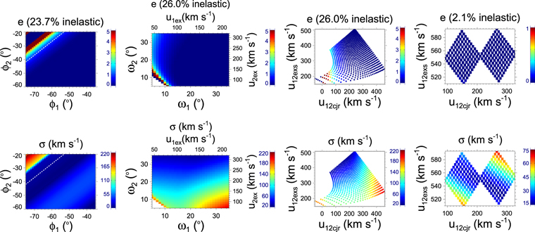
Figure 7. Same as Figure 4, but for the 2012 March 4–5 CMEs.
Download figure:
Standard image High-resolution imageThe errors in the angular half-width of the CMEs also suggest that the probable nature of the collision is perfectly inelastic. Similar to the other cases described above, the ratio of the CME2 to CME1 expansion speeds is significantly higher for values of e > 1 than that for e < 1 (second panel of Figure 7). In the different samples of data points having values of  /
/ from greater than 1 to 4, the percentage of data points with e > 1 among those samples increases from 11.1% to 80.9%., i.e., the probability of e > 1 increases with the increasing ratio of
  to
to  . The errors in the initial speeds also give a significantly larger probability for perfectly inelastic collision with no chance for super-elastic collisions. In Table 6, for the 2012 March 4–5 CMEs, the entry corresponding to e > 1 noted to be "NA," which refers to "Not Applicable," i.e., no data points or no probability is found for e > 1. From the speed uncertainties, there are no points having values of 0 < e < 1 with
  greater than three times
  . This means that as the ratio of
  to
to  becomes greater than 1 to 3, the probability of inelastic collisions decreases from 100% to 0%. Despite taking the uncertainties listed in the fourth row of Tables 4–6, we always note a smaller probability for inelastic (0% to 25.9%) or super-elastic (0 to 10.5%) collisions, and therefore, the collision of the 2012 March 4–5 CMEs is determined to be perfectly inelastic.
3.5. 2012 November 9–10
The characteristics of the collisions of the 2012 November CMEs are mentioned in Table 3 and suggest perfectly inelastic collision. The values of e and σ estimated by taking the uncertainties in the CME parameters are shown in Figure 8. This is consistent with the study by Mishra et al. (2015a) where they considered the head-on collision scenario. The probability of a different nature of collision and the characteristics of the CMEs due to the uncertainties in their propagation directions, angular sizes, and initial speeds are given in Tables 4–6. From the tables, we note that the uncertainties of ±20° in the propagation directions cause a decrease in the probability of perfectly inelastic collision of up to 48.3%; however, this remains higher than any other nature of collision.
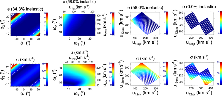
Figure 8. Same as Figure 4 but for the 2012 November 9–10 CMEs.
Download figure:
Standard image High-resolution imageGiven the uncertainties in the angular widths, we have several data points for e corresponding to different pairs of widths. We note that in the different samples of data points having values of  /
/ from greater than 1 to 4, the probability of having e > 1 (i.e., super-elastic collisions) among those samples increases from 2% to 100%. From Table 5, the probability of inelastic collision is 58%, and among this around one-third correspond to e values less than 0.1 and the probability of a perfectly inelastic collision is 40.7%. The inelastic and super-elastic values of e comes from much smaller values of the angular width of CME1 than that of CME2. This is in contrast with the observations where the CME1 angular half-width is around three times the CME2 angular half-width. Taking the errors in the speeds also gives the probability of 100% for perfectly inelastic collision. It is also clear from the third panel of Figure 8 that a low approaching speed leads to a larger probability for super-elastic collision. Carefully looking at the variations of the e and σ values together while keeping in mind the observed CME parameters, we attribute a perfectly inelastic nature of collision to the CMEs of 2012 November 9–10.
3.6. 2013 October 25
Under the oblique collision scenario, the characteristics of the 2013 October 25 CMEs at the beginning of the collision and the collision parameters are listed in Table 3. The nature of collision is found to be at the boundary of inelastic and super-elastic, i.e., perfectly elastic. This value of e is slightly different from the study of Mishra et al. (2016), where a different angular width (i.e., expansion speed) of the CMEs was considered. However, similar to the other analyzed cases described above, before decisively attributing a particular nature of collision to any CME, we assess the uncertainty in the estimated e value. Figure 9 shows the variation in e and the corresponding σ value against the uncertainties in the observed CME directions, angular half-widths, and speeds. The effects of these uncertainties on the CME characteristics and collision parameters are listed in Tables 4–6. From the first panel (from the left) of Figure 9, it is clear that e = 0 gives exceptionally large (i.e., 180 to 250 km s−1) values of σ, which are not reliable as they also violate the momentum exchange condition. The increase in the separation angle between the CMEs over that determined from the GCS model, i.e., an increase in the longitude of one CME and a decrease in another, shifts the nature of the collision into the super-elastic regime with only a small probability for inelastic collision. However, the maximum value of σ (i.e., 163) for super-elastic collisions is almost three times larger than that obtained corresponding to the inelastic regime.

Figure 9. Same as Figure 4, but for the 2013 October 25 CMEs.
Download figure:
Standard image High-resolution imageFrom Table 5, the uncertainties in the angular width of the CMEs shift the nature of the collision into the inelastic regime (with a probability of 75%) to a great extent. The second panel of the figure shows (similar to other cases) that the collision tends to be super-elastic in nature when the expansion speed of the following CME becomes larger while the expansion speed of the preceding CME becomes smaller. We note that the values of  /
/ reach the maximum value of up to 7.5 for e > 1, while it reaches the maximum value of 2.7 for 0 < e < 1. The probability of e > 1 increases from 32.1% to 100% as the values of
  /
/ become greater than 1 to 3. The fourth panel of the figure and the sixth row of Table 6 show that the uncertainties in the initial speeds of the CMEs give around equal probabilities for an inelastic and a super-elastic collision with no obvious difference in σ ranging from 5 to 100 km s−1. The values of e for the inelastic regime also range from 0.5 to 0.9, and thus are never close to e = 0. Further, we note that among the points where the values of
  is larger than three time the values of
  , around 99.1% of the points show e > 1. We decide that the probable nature of collision of the 2013 October 25 CMEs may vary from inelastic to super-elastic under reasonable uncertainties in the observed directions, widths, and speeds of the CMEs.
3.7. 2011 August 3–4
Using the observed CME parameters, the value of e is estimated to be 0.1. The parameters derived from the propagation and expansion speeds of the CMEs and collision parameters are noted in Table 3. The effect of the ±20° uncertainties in the directions of the CMEs on the values of e and σ is shown in the first panel of Figure 10 and in the seventh row of Table 4. We note that around 4.6% of the data points violating the momentum exchange condition correspond to e = 0, and therefore they are unreliable. There is a larger probability of 76.6% that the collision would be inelastic with a lesser value of σ ranging between 30 and 40 km s−1.
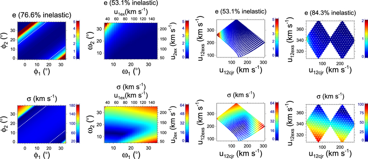
Figure 10. Same as Figure 4, but for the 2011 August 3–4 CMEs.
Download figure:
Standard image High-resolution imageThe effect of the uncertainties on the angular half-width of the CMEs is listed in Table 5 and shown in the second and third panels of Figure 10. We note that it is more likely that values of e > 1 correspond to a larger value of the ratio of the CME2 to CME1 expansion speeds before collision than values of e < 1. We also found that among the points where the values of  are greater than the values of
  , around 11.8% have e > 1. Among the data points where
  is greater than six times
  , around 100% of the points have e > 1. This shows that a super-elastic collision is probable with a low relative approaching speed of the CMEs. Among all of the data points having 0 < e < 1, around 92.1% of them have a larger value of
  than
than  . The effect of the uncertainties on the speed is shown in the seventh row of Table 6 and fourth panel of Figure 10. From here we find that the probability of super-elastic collisions increases as the relative approaching speed of the CMEs decreases. There is a probability of around 84.3% for an inelastic collision with the σ value always less than 100 km s−1, and thus it is reliable. From the results shown in the figures and the tables, we decide that the nature of collision of the CMEs of 2011 August 3–4 is inelastic.
3.8. 2012 September 25–28
For the CMEs of 2012 September 25 and 28, the value of e = 2.0 is found for an oblique collision, and the corresponding CME characteristics are listed in Table 3. Assuming the head-on collision scenario in Mishra et al. (2015b), the value of e is found to be 0.8, which is obviously underestimated compared to that from the oblique collision scenario. The effect of the errors on the propagation directions, angular widths, and speeds on the values of e and σ is listed in Tables 4–6, respectively. The characteristics of the CMEs derived from their expansion and propagation speeds for different natures of collision are listed in these three tables. By ignoring the points violating the momentum exchange condition and larger values of σ while taking the uncertainties in the directions of the CMEs, we note a dominant probability of around 89.8% for a super-elastic collision (first panel of Figure 11).

Figure 11. Same as Figure 4, but for the 2012 September 25–28 CMEs.
Download figure:
Standard image High-resolution imageThe second panel of Figure 11 shows that e > 1 is more probable with an expansion speed of the following CME larger than that of the preceding CME. For instance, the values of  /
/ reach a maximum of up to 7.2 for e > 1, while its maximum is 1.44 for 0 < e < 1. The third panel of the figure shows that a decrease in the relative approaching speed (
 ) of the CMEs increases the probability of a super-elastic collision. In three different samples of data points, each having the ratio of
  to
to  greater than 1, 2, and 3, the probability of e > 1 among these samples is 74.1%, 99.7%, and 100%, respectively. However, around 48.1% of the samples among the points having 0 < e < 1 values have larger values of
  than
than  . The eighth row in Table 6 and the fourth panel of Figure 11 suggest almost equal probabilities for a super-elastic and an inelastic collision. However, the values of e for an inelastic nature of collision is always greater than 0.5. Given reasonable errors in the directions, sizes, and speeds of the CMEs of 2012 September 25–28, it is difficult to ascertain a particular collision nature, as the most probable varies from the inelastic to a super-elastic regime.
4. Results
The results of our analysis of a total of eight cases of interacting CMEs are organized into two parts. The physical nature of the collision obtained using the observed parameters of the CMEs is summarized in Section 4.1. We pay attention to the relative values of the CME parameters before and after collision, for all cases. In this section, we also compare different cases of the observed CMEs to find a dependence of the CME parameters on a particular physical nature of collision (Table 3). In Section 4.2, the results from taking the uncertainties in each individual case are summarized. Here we emphasize that the uncertainties in the kinematic parameters of the CMEs influence the calculated value of the coefficient of restitution (e), and thus, it is a mathematical outcome (Tables 4–6). Such an analysis of uncertainties suggests that the errors in some of the parameters of the CMEs would affect the calculated value of e, i.e., the nature of collision. Such mathematical influences on the calculated nature of collision for selected colliding CMEs do not imply a real change in the physical nature of the collision of those selected CMEs. Hence, the mathematical uncertainties in individual cases of CMEs no longer represent the same physical CMEs as observed. Therefore, a mathematical treatment as performed in our study does not indicate any real change in the CME parameters that affect the physical nature of the collision.
4.1. Nature of Collision: Results from the Observed Parameters of the CMEs
In the oblique collision scenario, we have studied several cases of colliding CMEs using their geometrical, kinematic, and mass estimates from multiple-viewpoint remote observations. The important results without considering the uncertainties in the measured CME parameters are noted in Table 3 and shown in Figure 12. On careful inspection of the figure, we notice that four data points in the inelastic regime (i.e., November, March, August, and June) in the bottom panel of Figure 12 show a pattern of decreasing approaching speed with increasing value of e. Another four data points in the elastic to super-elastic regimes (i.e., 2013 October, 2010 May, 2011 February, and 2012 September) may be considered to have an almost constant approaching speed with increasing value of e. A similar trend for the data points divided into two populations can be noted in the middle panel of the figure. However, unlike the middle and bottom panels, in the top panel of the figure, the data points do not represent two separate populations. None of the data points of any one population could be considered as obvious outliers as they are not unusually far from other data points. Further, all eight data points representing eight selected cases of interacting CMEs do not have the same precision. This is because our analysis using available single- or multiple-view point observations have determined the CME parameters for different cases with different accuracies (Table 1). Also, the different estimated parameters may have different precisions even for a particular case of interacting CMEs. For example, as described in Section 2.1.3, the collision duration of the 2010 May CMEs have a large uncertainty, while we do not expect a large uncertainty for its pre-collision speed measurements. Similarly, the CMEs of 2012 March 4–5, propagating largely at different latitudes, hardly satisfy our assumptions of a collision scenario in the ecliptic plane, as described in Section 2.1.4, and are expected to have large errors in speed measurements but no large errors for the collision duration. In light of the aforementioned notes, we avoid using any outlier detection scheme for our extremely limited number of data points. We opine that a significant portion of the data (i.e., around 50%) cannot be considered and are excluded as collective outliers, and thus we prefer to investigate each data point individually.
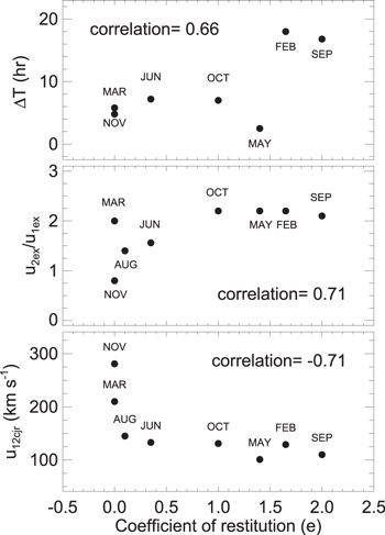
Figure 12. Values of the coefficient of restitution shown on the X-axis in all the panels. The collision duration, ratio of the pre-collision expansion speed of CME2 and CME1, and relative approaching speed of the CMEs along the line joining their centroids are shown on the Y-axis of the top, middle, and bottom panels, respectively.
Download figure:
Standard image High-resolution imageAmong the cases studied using their observed parameters, two cases (CMEs of 2012 June 13–14 and 2011 August 3–4) show inelastic collisions and two cases (CMEs of 2012 March 4–5 and 2012 November 9–10) show perfectly inelastic collisions. One case (CMEs of 2013 October 25) shows elastic collision, and three other cases (CMEs of 2011 February 14–15, 2010 May 23–24 and 2012 September 25–28) show super-elastic collisions. The super-elastic collision shows a collision duration as large as 18 hr for the 2011 February 14–15 CMEs to as small as 2.5 hr for the 2010 May 23–24 CMEs. However, the collision duration of the 2010 May CMEs has large errors as it is derived using only STEREO-A observations due to a large data gap in STEREO-B just after the beginning of the collision (Lugaz et al. 2012). It is also noted that the super-elastic collisions occur as close as 24  up to as far as 170
  from the Sun. The bottom panel of Figure 12 indicates that the coefficient of restitution (e) is negatively correlated (correlation coefficient = −0.71) with the relative approaching speed. From the middle panel, it is found that e is positively correlated (correlation coefficient = 0.71) with the ratio of the CME2 to the CME1 expansion speeds. The top panel shows that the e value is positively correlated (correlation coefficient = 0.66) with the collision duration of the interacting CMEs. We understand that a relatively better correlation could have been found if the errors in measured speeds and collision duration were smaller for the 2012 March and 2010 May CMEs, respectively. Also, the data points for the 2013 October, 2010 May, 2011 February, and 2012 September cases indicate that the long interval of collision duration favor, to some extent, determining a larger value of e. However, we emphasize that Figure 12 does not show a one-to-one correlation between the measured parameters and e values. Thus, the e value probably depends on several parameters and their relative contribution could not be assessed in the present study.
To understand the interrelatedness of several parameters as listed in the columns of Table 3 for all events, we carried out a principal component analysis (PCA; Hotelling 1933; Jolliffe 2002), and the findings are given in Appendix B. The analysis gives two significant variables, PC1 and PC2. A higher value of PC1 comes from a combination of an increase in the coefficient of restitution (e), post-collision relative separation speed ( ), ratio of the CME2 to CME1 expansion speeds (
 /
/ ), and a decrease in the pre-collision relative approaching speed (
 ). Large values of PC2 primarily show a decrease in the sum of expansion speed (
 ), and, second, a decrease in the values of the direction of impact (ψ) and distance (R) of the collision site. From the bottom panel of Figure 13, we deduce that the CMEs of 2011 February 14–15 and 2012 September 25–28 showing super-elastic collision have larger values of PC1, i.e., they have larger
  /
/ and
and  while having smaller
  . This is also evident from Table 3, where
  ranges between 100 and 280 km s−1 while its value for e > 1 ranges only between 100 and 130 km s−1. Further, the value of
  for super-elastic collisions is greater than 135 km s−1 while it is less than 45 km s−1 for inelastic collision. We also note a weak negative correlation between
  and e values. The CMEs of 2012 June 13–14 and 2011 August 3–4 have lower approaching speeds of 135 km s−1 and 145 km s−1, respectively, but they show inelastic collisions, which are largely away from elastic collision. This is because of the fact that these CMEs also have a lower value of
  /
/ and
and  , with a higher
  value. The CMEs of 2012 March 4–5 have a large value of
  /
/ of 2.0, but also have a large value of
  , and therefore show perfectly inelastic collision. Thus, we suggest that a super-elastic collision of the CMEs is expected with a smaller
  and simultaneously larger
  /
/ , which together lead to a larger
  value.

Figure 13. Output from principal component analysis (PCA). From top to bottom, the first panel shows the loadings of the variables on two principal components, PC1 with red and PC2 with green. The second panel shows the variations of the factor scores of the observations (for the CME cases of 2011 February, 2012 June, 2010 May, 2012 March, 2012 November, 2013 October, 2011 August, and 2012 September as listed in Table 1) on PC1 and PC2.
Download figure:
Standard image High-resolution image
Succinctly, among the eight cases studied (Table 3), we find no clear dependence on the direction of impact, distance of collision site, and mass ratio of different cases of the CMEs for a particular type of collision. However, some dependence of e on the propagation direction of CMEs is noted from the mathematical analysis described in Section 4.2. From the table, it is highlighted that the value of e primarily depends, in order of priority, on  ,
,  /
/ , ΔT, and
  . Although our study is a first attempt at taking several cases of interacting CMEs, the results are limited to a large extent in the absence of enough observed cases of interacting CMEs to be analyzed for a statistically significant multiparameter study. We also notice that the value of the coefficient of restitution (e) is underestimated in the head-on collision scenario compared to the oblique collision scenario. Our analysis suggests that the pre-collision speeds of the centroids of CMEs (i.e., a combination of leading edge and expansion speeds) must be used in the scheme of forecasting the collision nature of CMEs.
4.2. Role of Uncertainties in the Observed Parameters of the CMEs
The results obtained by considering the uncertainties in the observed propagation directions, leading edge speeds, and angular widths (i.e., expansion speeds) of the CMEs are noted in the Tables 4–6, respectively. We attempt to understand how the uncertainties lead to different probabilities for different types of collision for any selected case of interacting CMEs. The considered uncertainties in the propagation directions of the 2012 March and 2012 November CMEs give a likelihood of perfectly inelastic collision of around 62% and 48%, the uncertainties in their angular widths give a likelihood of perfectly inelastic collision of around 65% and 41%, and the uncertainties in their speeds give a likelihood of perfectly inelastic collision of around 98% and 100%, respectively. Similarly, the uncertainties in the propagation directions of the 2012 June and 2011 August CMEs give a likelihood of inelastic collision of around 65% and 77%, the uncertainties in their angular widths give a likelihood of inelastic collision of around 50% and 53%, and the uncertainties in their speeds give a likelihood of inelastic collision of around 94% and 84%, respectively. For the 2013 October CMEs, the uncertainties in the propagation directions, widths, and speeds correspond to a probability of 67% for super-elastic collision, 75% for inelastic collision, and 50% for super-elastic collision, respectively. The uncertainties in the directions of the 2011 February, 2012 March, and 2012 September CMEs give a likelihood of super-elastic collision of around 88%, 38%, and 89%, the uncertainties in their widths give a likelihood of super-elastic collision of around 73%, 43%, and 60%, while the uncertainties in their speeds give a likelihood of super-elastic collision of around 89%, 61%, and 49%, respectively.
From the above values of probabilities and the values of e shown in Figures 4–11, we note that the effect of the uncertainties is so large for some cases that it is difficult to ascertain a particular nature of collision for those cases. For instance, under the uncertainties considered, three cases (CMEs of 2010 May 23–24, 2013 October 25, and 2012 September 25–28) of the CMEs show the most probable nature of collision vacillating between the inelastic to super-elastic regime. Such an effect is expected for the CMEs of 2013 October 25 as its observed nature of collision was elastic, i.e., at the boundary of the inelastic and super-elastic. However, the CMEs of 2010 May show huge uncertainties in the e value in their directions, widths, and speeds. The CMEs of 2012 September 25–28 show a large deviation from the super-elastic nature due to uncertainties in the pre-collision leading edge speeds of the CMEs. Such uncertainty in the e value due to a change in the speed of the CMEs was not noted in Mishra et al. (2015b). We point out that in the oblique collision scenario, even a reasonable uncertainty in the observed CME characteristics leads to a different nature of collision. The e value is found to be dependent to some extent on the relative propagation directions of the CMEs. However, this was not recognized in earlier studies that assumed the head-on collision scenario (Mishra et al. 2014, 2015a). We envisage that a change in the propagation directions may lead to a change in the relative contribution of the expansion speeds to the centroids speeds of the CMEs along the line joining their centroids. We did not make any attempts to understand whether the different propagation directions of the CMEs, which cause different contact areas between them, have some role in deciding the nature of the collision. The selected cases of CMEs that have larger variations in their e values are those with the moderate as well as the lowest assigned accuracies as mentioned in Table 1. Therefore, we think that it is not solely the accuracy of the estimated pre- and post-collision kinematics that makes the value of e more sensitive to the observed CME parameters.
From the fourth and fifth columns of Table 5, we note a larger value of the ratio of the CME2 to CME1 expansion speeds ( /
/ ) for super-elastic collisions (e > 1) than for e < 1, for all of the CME cases. This is evident from the second panel (from the left) of Figures 4–11. However, the column in Table 6 corresponding to the uncertainties in the initial speeds of the CMEs shows no significant difference in the value of
  /
/ for super-elastic and inelastic collisions. The sixth and seventh columns of Table 5 show that as the ratio of the summation of the expansion speed (
 ) to the relative approaching speed (
 ) increases, the percentage of points (i.e., probability) having e > 1 increases. This implies that a decrease in the approaching speed of the interacting CMEs increases the probability of super-elastic collision. This is also evident from the third panel of Figures 4–11. The fourth panel of Figures 4–11, which corresponds to uncertainties in the initial speeds of the CME leading edges, also shows that a small value of the relative approaching speed of the centroids of the CMEs favors the occurrence of super-elastic collision. The last columns of Tables 5 and 6 suggest that there remains a certain probability for inelastic collision despite the approaching speed being smaller than the summation of the expansion speeds of the CMEs.
5. Discussion
In an earlier analysis, it was established that the uncertainties in the masses of the CMEs hardly has any effect on the collision nature of the CMEs (Shen et al. 2012; Mishra & Srivastava 2014; Mishra et al. 2015b, 2016). This is expected from our approach, as the observed post-collision speeds ( ) of the centroids of the CMEs are modified to determine their expected values (
 ), which will be used to estimate the value of e while being constrained by momentum conservation. Therefore, in the present analysis, we did not assess the effect of the uncertainties on the mass. Instead, our analysis focused on uncertainties in the other CME parameters. However, we do admit that the mass estimated in the COR field of view may not be the actual mass at the collision sites. This is possible due to the well-known snow plough effect (DeForest et al. 2013; Feng et al. 2015). Further, it is difficult to know whether the total masses of the interacting CMEs participate in a collision where only part of the CME gets in contact with the other. The assumptions of a spherical structure for the CMEs and the mass centered at the centroid of the CMEs are idealistic, but are nevertheless pragmatic for such studies.
Among the eight selected cases in our study, the SSSE method could be applied in five cases, and thus, their propagation directions could be estimated in the HI field of view. We note that the direction estimates from SSSE using two viewpoints of STEREO are less reliable than those from the GCS model, which uses an additional viewpoint from SOHO. Therefore, we used the directions estimated from the GCS model in the COR field of view to study the collision. This is also because during the time of occurrence of the selected CMEs (except for 2010 May 23–24), the separation between both STEREO spacecraft is either close to 180° or greater than this. For such a separation of the STEREO spacecraft, the direction estimates from SSSE have large errors and noise as described in earlier studies (Liu et al. 2010a, 2013; Mishra et al. 2014; Mishra & Srivastava 2014; Liu et al. 2016). When STEREO-A and B are at anti-parallel directions, a singularity occurs when implementing the SSSE method results in a larger uncertainty in the directions even with a smaller uncertainty in the elongation measurements of the CMEs (Liu et al. 2011; Mishra & Srivastava 2013). The estimated directions from SSSE are within 10° of those derived from GCS for the 2010 May, 2012 March, and 2012 June CMEs. The disagreement between the GCS- and SSSE-derived directions is larger at around 20° for 2011 February and 2011 August cases. In our analysis, we assess the effect of the ±20° uncertainties in the directions on the nature of collision. Including the errors in the tracking of the CMEs in the HI field of view and the errors from the reconstruction methods (Liu et al. 2010a; Davies et al. 2013; Liu et al. 2013; Mishra et al. 2015b; Vemareddy & Mishra 2015), we believe that the observed speeds also have uncertainties and their effects are examined in our study.
We compared the remotely derived post-collision speed values with the measured speeds from in situ observations to infer the errors from the remote measurements. We notice a significant disagreement between two sets of observations for the 2011 February, 2012 June, 2012 September and 2013 October CMEs. In short, the speed measured in situ is smaller than the speed values derived from remote observations by 270 km s−1 for CME1 and by 140 km s−1 for CME2 in the 2012 June case, by 400 km s−1 for CME1 and by 100 km s−1 for CME2 in the 2012 September case, and by 150 km s−1 for the 2013 October CMEs. The overestimation of the speed for the 2012 June, 2013 October, and 2012 September CMEs from the SSE or SSSE method implemented in the remote observations is expected as these CMEs are receding from the observers STEREO-A and B (Liu et al. 2013; Mishra et al. 2015b). Also, the propagation direction of the 2013 October CMEs suggests a flank encounter with the in situ spacecraft, and this is an additional reason for the discrepancy between the remote and in situ measured speed values for this case. The in situ measured speed of the 2011 February CMEs is 100 km s−1 larger than its post-collision speeds measured from remote observations. This is possible if the CMEs overexpand before reaching L1. The remotely measured kinematics and its connection with the in situ measured values and the disagreement therein for the CMEs of 2011 February 14–15, 2010 May 23–24, 2012 November 9–10, and 2012 September 25–28 are discussed in earlier studies of Lugaz et al. (2012), Mishra & Srivastava (2014), and Mishra et al. (2015a, 2015b), respectively.
The large discrepancy between the remote and in situ measured post-collision speeds may reduce the accuracy of our analysis of the nature of collision of the cases (e.g., 2012 September 25–28 and 2012 June 13–14 CMEs) where the CMEs have little or no chance of having a flank encounter with the in situ spacecraft, and collision takes place largely away from the Sun. The appraisal of errors in our analysis would be difficult as the errors in the pre-collision speeds of the CMEs cannot be inferred from a comparison of remote and in situ measurements. If there is an equal proportion of errors in the pre- and post-collision speeds, then they get nullified by one another in the calculation of the coefficient of restitution. We note that the SSSE reconstruction method implemented in the HI observations of the 2012 September CMEs have overestimated the remotely measured post-collision speed of CME1 to a greater extent than that of CME2. This implies that it is likely that not as much momentum was transferred to CME1 as is found from the kinematics profiles and used for analysis. It is therefore very likely that this event was not as super-elastic (or not at all) as what was found in our analysis using the oblique collision scenario. This agrees with the results listed in Table 6, where this event shows a likelihood of 50% for inelastic collision with ±100 km s−1 uncertainties in the observed post-collision speed. Similarly for the case of the 2012 June CMEs, the SSSE method overestimated the post-collision speed of CME1 to a greater extent than that of CME2. Therefore, the nature of collision of this case could have shifted further toward close to perfectly inelastic. Therefore, this approach should be used to ascertain only a finite probability for a particular nature of collision. We also keep in mind that the possibility of errors in the speeds derived using remote observations cannot be excluded based only on good agreement between two sets of remote and in situ observations. This is because of the difficulty in accurately quantifying the possible deceleration, acceleration, deflection, and overexpansion of the CMEs beyond the collision site, and the trajectory of the in situ spacecraft through the CME. Thus, it is possible that complex interactions during the Sun-to-Earth propagation may not be revealed by in situ measurements alone. Further, the inconsistency in speed values between remote and in situ measurements may be partially due to the fact that a remotely tracked feature of a CME has not been intercepted by the in situ spacecraft.
For all selected cases, we noticed a deceleration of the leading edge of the following CME well before an acceleration of the leading edge of the preceding CME. This is partly because the preceding CME may act as a magnetic obstacle for the following CME (Temmer et al. 2012; Mishra & Srivastava 2014), and thus a remote interaction between them starts before the actual collision takes place. This is also partly because a thrust from the following CME on the rear of the preceding CME requires some time (i.e., the minimum Alfvènic crossing time for the CME) to arrive at its leading edge. We also point out that the identification of the collision phase based on the observed exchange in kinematics of the CMEs' leading edges may involve errors and creates uncertainties in our analysis. The marked start of the collision in our study is later than the actual contact between the CMEs as described in Mishra et al. (2016). This leads to an overestimation of e to some extent, which may be nullified by an underestimation of e caused by ignoring the contribution of the CME2-driven shock to accelerate CME1 in our study. Such errors causing competing effects of over- and underestimation of the value of e need to be explored further. It is expected that a collision phase is complex, involving different timescales for the compression by shock, subsequent expansion, exchange of momentum, and magnetic reconnection. Therefore, we do realize that large-scale magnetically structured plasmoids would not collide as ordinary objects.
Some separation between the leading edge of the preceding and following CMEs at the beginning of the collision is expected due to the finite size of the preceding one. Carefully inspecting the estimated distance profiles of the leading edge of the CMEs for four cases (i.e., 2011 February, 2012 June, 2013 October and 2011 August), we note that the separation is within 5 R⊙. However, this separation ranges from 20 R⊙ to 25 R⊙ for four other cases (i.e., 2010 May, 2012 March, 2012 November, and 2012 September). The obtained separation between the leading edge of CME2 and CME1 implies a much smaller diameter of CME1 than reported for CMEs in earlier studies (Leitner et al. 2007; Gulisano et al. 2010; Wang et al. 2015). It is understood that the separation between the leading edges of CME2 and CME1 depends not only on the size of CME1 but also on their propagation directions. Thus, a direct inference of the size of the preceding CME from only the separation between the leading edges of colliding CMEs may be inaccurate in the case of oblique collision where projection effects may be significant. Further, it is difficult to ensure that the tracked features of the CMEs in the J-maps correspond to the outermost portion of the CMEs. Also, the possible compression of the colliding CMEs may prevent us from measuring the exact diameter of CME1. Taking all these points into account, the inferred smaller size of the preceding CME is not that surprising. However, when including the possibility of errors in marking the collision phase, the inferred smaller size of CME1 may imply that the beginning of the collision should be marked a little earlier. Due to this fact, the value of e would be overestimated to some extent in our analysis, where the collision phase is marked by noting the speed variations of the CMEs rather than the separation between their measured leading edges.
CME–CME interaction is actually a three-dimensional phenomenon. Although the kinematics of the CMEs is estimated using the SSE or SSSE methods of 3D reconstruction, the J-maps are made along the ecliptic only. This means that the kinematics used even in the oblique collision scenario represents the collision of only part of the CMEs, as Temmer et al. (2014) showed that colliding CMEs have different speeds at different position angles. In our study of the cases where the SSE method is used, neither the post-collision directions nor deflection of the CMEs during collision is used for estimating their observed speeds. However, while solving the equations for the collision, we determined the post-collision directions and modified the observed post-collision speeds for collision analysis. The theoretical estimate of the expected post-collision speeds for the analysis suggests that the deflection of the CMEs cannot be completely overlooked. Since the elongation measurements for an observer and the observed propagation directions of the CMEs are linked, the true effect of a change between the pre- and post-collision directions on the speed is difficult to assess. Further, we have not considered the possible rotation and deflection of the CMEs, and focus instead on the linear speeds of the centroids. Also, we have ignored the contribution of the solar wind in the acceleration or deceleration of the CMEs during the collision phase (Shen et al. 2012, 2013). Such assumptions probably lead to significant errors for CMEs like those of February 14–15 and September 25–28, which have significantly longer collision phases. Neglecting the effect of solar wind probably induces errors in the 2011 August 3–4 CMEs where their post-collision speeds are derived from the in situ observations while the collision occurred around 145 R☉ from the Sun.
From our analysis of the observed cases of the CMEs, it is clear that an expansion speed of the following CME significantly larger than the preceding one contributes to reducing the relative approaching speeds of the centroids of the CMEs. The larger expansion speed of the following CME implies a larger internal pressure inside (Wang et al. 2009) and probably refers to a hardening of the CMEs. It has been found in experiments that a collision of hard ceramic spheres with softer polycarbonate plates (Louge & Adams 2002; Kuninaka & Hayakawa 2004) is super-elastic in nature. It seems that some of the magnetic and thermal energies of the following CMEs get converted into macroscopic kinetic energy of the CMEs to make the collision super-elastic. We are inclined to propose that the internal pressure of CMEs indirectly displays the physical nature of macroscopic expanding plasma blobs. Therefore, the different physical characteristics of the CME plasma may lead to different types of collision. The fair dependence of the nature of collision on the duration of collision obtained in our study possibly indicates a role for plasma processes in CME–CME collision. The long duration of collision is meant to show super-elastic collision where additional kinetic energy would have been produced through magnetic reconnection. A thorough understanding of the physics and plasma processes responsible for super-elastic collision may involve the role of magnetic pressure and the orientation of flux ropes of the CMEs (Lugaz et al. 2013). Despite doing extensive data analysis for a total of eight cases, we could not establish a sufficient condition for super-elastic collision to occur. Several limitations of such a study using imaging observations are discussed in earlier studies (Shen et al. 2012; Lugaz et al. 2013; Mishra et al. 2016).
To address some of the limitations related to CME-driven shock (Vandas et al. 1997; Lugaz et al. 2005), the heating, compression (Shen et al. 2013, 2016), roles of reconnection and overexpansion (Lugaz et al. 2013), and numerical simulations of such CMEs may be helpful. Understanding the role of oblique collision of CMEs in deciding their deflection and elasticity using simulation studies (Schmidt & Cargill 2004; Xiong et al. 2009) is also required. It is possible to get some clues to the physical processes during the collision if there are some in situ measurements of the CME plasma in the collision site shortly before and after collision. The present study emphasizes only the probable nature of a collision, leaving room for uncertainties. An analysis of several cases by combining the simulations and observations for the same colliding CMEs is important for making progress in understanding the nature of collision of CMEs as well as space weather studies.
6. Conclusion
Our study emphasizes the possibility of a large uncertainty in the calculated value of the coefficient of restitution (e) from the observed CME characteristics. Such an uncertainty is not obviously noticed when considering the head-on collision scenario where the value of e is often underestimated. This is evident, however, when taking into account the uncertainties for the oblique collision scenario, as the nature of collision of three (i.e., 2010 May, 2013 October, and 2012 September CMEs) of the eight cases of CMEs could not be ascertained decisively. We suggest that the nature of collision of the CMEs can only be determined with a finite probability for a specific nature. We note that the direction of impact, distance of collision site from the Sun, and mass ratio of the CMEs do not favor a particular nature of collision. The decrease in the pre-collision approaching speed of CMEs along the line joining their centroids and an increase in the ratio of the CME2 to CME1 pre-collision expansion speeds give a large probability for super-elastic collision. Our study concludes that the expansion speed of the following CME larger than that of the preceding CME, giving a relatively lower approaching speed before the collision and a higher separation speed after the collision, tends to increase the probability for super-elastic collision (Shen et al. 2012, 2016). Thus, the expansion speed of the CMEs plays a greater role than any other CME parameters. Our study shows the dependence of the calculated nature of collision on the propagation directions, angular sizes, and leading edge speeds of the CMEs. This is probably because these parameters of the CMEs indirectly alter the relative contributions of the expansion speeds to the leading edge speeds of the CMEs and thus to the relative approaching speeds of their centroids. However, these uncertainties in the CME parameters do not alter the physical nature of the collision for any of the selected cases. The physical processes probably responsible for converting the magnetic energy into kinetic energy of the CMEs, to make a collision super-elastic, need to be analyzed in detail.
We acknowledge the UK Solar System Data Center for providing the processed Level-2 STEREO/HI data. This work is supported by NSFC grant Nos. 41131065, 41574165, and 41421063. W.M. is supported by the Chinese Academy of Sciences (CAS) President's International Fellowship Initiative (PIFI) grant No. 2015PE015. We thank the referee for insightful comments. W.M. also thanks A. K. Awasthi and A. Raghav for helpful discussions.
Appendix A:
Our approach considers two successively launched CMEs (CME1 and CME2) having different angular half-widths ( and
and  ) propagating as expanding bubbles in two different directions (
 and
and  ) from the Sun−Earth line and along the propagating directions
  and
and  relative to the line joining their centroids at the instant of collision.
Thus, we will get
Using the usual notations and conventions used in this paper, for CME1,  and
and ![${u}_{1\mathrm{ex}}={u}_{1}\sin ({\omega }_{1})/[1+\sin ({\omega }_{1})]$](https://content.cld.iop.org/journals/0067-0049/232/1/5/revision1/apjsaa8139ieqn211.gif) . Similarly, it will be for CME2.The post-collision directions of propagation of the CMEs relative to the Sun−Earth line are
. Similarly, it will be for CME2.The post-collision directions of propagation of the CMEs relative to the Sun−Earth line are  and
and  , and they are
  and
and  relative to the line joining their centroids. With the theoretically determined expected post-collision speeds of the centroids (
 ) of the CMEs using a certain value for e, which together allow the momentum to be conserved for the collision, we obtain Equations (2)–(4):


For the oblique collision scenario considered, the speed of the centroid of CME1 along the line joining the centroids of both CMEs will be  = u1c
= u1c ) and similarly for CME2. For collision to occur,
  +
+ ![${u}_{2\mathrm{ex}}]$](https://content.cld.iop.org/journals/0067-0049/232/1/5/revision1/apjsaa8139ieqn220.gif)

 −
−![${u}_{1\mathrm{ex}}]$](https://content.cld.iop.org/journals/0067-0049/232/1/5/revision1/apjsaa8139ieqn223.gif) and
and  −
− 
 (
( +
+  ) must be satisfied. Using the above equations, the value of
  and
and  for a definite value of the coefficient of restitution (e) is determined. Thereafter, the expected values of the post-collision speeds of the leading edge of the CMEs (
 ,
,  ) are determined and compared with the leading edge speeds (v1, v2) as observed. The best-suited value of e is attributed to the nature of collision of the selected CMEs for which the deviation (i.e.,
 ![$\sigma =\sqrt{[{({v}_{1\mathrm{th}}-{v}_{1})}^{2}+{({v}_{2\mathrm{th}}-{v}_{2})}^{2}]/2}$](https://content.cld.iop.org/journals/0067-0049/232/1/5/revision1/apjsaa8139ieqn233.gif) ) between the observed and expected post-collision leading edge speeds is minimum. The pre-collision relative approaching speed and post-collision relative separation speed of the centroids of CME1 and CME2 are defined as
) between the observed and expected post-collision leading edge speeds is minimum. The pre-collision relative approaching speed and post-collision relative separation speed of the centroids of CME1 and CME2 are defined as  and
and  , respectively.
Appendix B:
To visualize the pattern of similarity/difference between the observation points and variables in Table 3, we used the most popular multivariate statistical method called PCA (Pearson 1901; Hotelling 1933; Jolliffe 2002). The method reduces the dimensionality of a data set while preserving as much "variability" (i.e., statistical information) as possible. The important information from the data set is expressed as a set of new uncorrelated orthogonal variables called principal components (PCs). Finding such new variables (PCs) reduces to solving an eigenvalue and eigenvector problem or singular value decomposition of the data matrix. The first principal component (i.e., PC1) is the axis that spans and captures the direction of most variation in the data. PC2 is the axis that spans the direction with the second most variation in the data, and similarly there are principal components for each variable (i.e., dimension) in the original data. Following the terminology of Abdi & Williams (2010), the value of the new variables (PCs) for the observations are called "factor scores." These "factor scores" are seen geometrically as the "projections" of the observations onto the principal components. Thus, a projection matrix having the eigenvectors of the data matrix in each row is used for "loadings" of the original variables on the PCs.
From Table 3, we take nine variables, e,  ,
,  /u1ex,
  ,
,  , ψ, ΔT, m2/m1, and R and denote them as a, b, c, d, e, f, g, h, and i, respectively, for all eight observations of the selected CME events. This data set made a data matrix of eight rows and nine columns. The nine eigenvalues for this data set are 3.96, 2.67, 1.32, 0.49, 0.32, 0.20, 0.02, 0, and 0, corresponding to the nine PCs associated with them. We note that PC1 and PC2, having eigenvalues greater than 2, account for 44% and 29.7% of the variance in the data, respectively. The other nine components (i.e., PC3 to PC9) taken together account for only 25% of the variations in the data. Therefore, we keep only the first two PCs for further consideration. The eigenvectors corresponding to the two eigenvalues represent the loading of the variables on PC1 and PC2. The loading of all nine variables, i.e., from a to i on PC1 is [0.48, −0.16, 0.40, −0.40, 0.50, 0, 0.35, 0.24, 0.03] and shown in red in the top panel of the Figure 13. The higher the loadings, the more important that variable is to the component. This shows that PC1 contrasts variable d with variables a, c, and e, as well as capturing the variations in these variables. Similarly, the loadings of the variables on PC2 are [0.12, −0.54, −0.11, 0.12, 0.06, −0.52, 0.04, −0.37, −0.51] and are shown in green in the top panel of Figure 13. PC2 captures the variations in the variables b, f, and i. Using the loading of the variables, we determined the factor scores of all eight observations (i.e., CME events from Feb 14–15 to Sep 25–28 as noted in Table 1) on PC1 and PC2. The obtained factor scores on these first two PCs are displayed in the bottom panel of Figure 13. The result derived from this analysis is emphasized in Section 4.1.