


Abstract
Measuring the distance of quasar outflows from the central source (R) is essential for determining their importance for active galactic nucleus feedback. There are two methods to measure R: (1) a direct determination using spatially resolved integral field spectroscopy (IFS) of the outflow in emission and (2) an indirect method that uses the absorption troughs from ionic excited states. The column density ratio between the excited and resonance states yields the outflow number density. Combined with a knowledge of the outflow's ionization parameter, R can be determined. Generally, the IFS method probes an R range of several kiloparsecs or more, while the absorption method usually yields R values of less than 1 kpc. There is no inconsistency between the two methods as the determinations come from different objects. Here we report the results of applying both methods to the same quasar outflow, where we derive consistent determinations of R ≈ 5 kpc. This is the first time that the indirect absorption R determination is verified by a direct spatially resolved IFS observation. In addition, the velocities (and energetics) from the IFS and absorption data are found to be consistent. Therefore, these are two manifestations of the same outflow. In this paper we concentrate on the absorption R determination for the outflow seen in quasar 3C 191 using Very Large Telescope/X-shooter observations. We also reanalyze an older absorption determination for the outflow based on Keck/High Resolution Echelle Spectrometer data and find the revised measurement to be consistent with ours. Our companion paper details the IFS analysis of the same object.

Original content from this work may be used under the terms of the Creative Commons Attribution 4.0 licence. Any further distribution of this work must maintain attribution to the author(s) and the title of the work, journal citation and DOI.
1. Introduction
Active galactic nucleus (AGN) feedback serves as an important link in the coevolution of supermassive black holes (SMBHs) and their host galaxies. It has thus become an essential feature of modern theories of galaxy formation (e.g., A. Cattaneo et al. 2009; J. Silk & G. A. Mamon 2012; J. Hlavacek-Larrondo et al. 2024) and state-of-the-art cosmological simulations (e.g., Y. Dubois et al. 2012; R. Davé et al. 2019; M. Donnari et al. 2021). In the quasar mode of AGN feedback, powerful outflows are driven by SMBHs accreting close to the Eddington limit. The energy and momentum carried by these outflows can be redeposited in the surrounding medium and thus contribute to various feedback processes. To assess this contribution quantitatively, it is important to determine the spatial extent of the outflowing gas (R), its mass (M), its mass flow rate (), and its kinetic luminosity () from observations.


Observational signatures of quasar outflows are detected primarily (a) in emission, as spatially resolved galactic-scale winds studied using integral field spectroscopy (IFS) (and other techniques such as long-slit spectroscopy), and (b) in absorption, as blueshifted troughs in the quasar spectrum observed as a result of the intersection of our line of sight with the outflowing gas. Both of these analysis techniques have been utilized greatly over the last two decades for their distinct advantages. Absorption analysis is much richer in spectroscopic information and has thus allowed the study of a wide range of physical parameters (e.g., density and ionization state) in the outflows. The detection of absorption troughs from metastable excited states plays a crucial role in the analysis as their population ratio with the resonance state is a reliable indicator of the outflow's number density. The ionization state is typically determined through a detailed photoionization modeling of the outflow, and combined with the number density leads (using Equation (4)) to an indirect determination of the distance of the outflow from the central source (e.g., M. de Kool et al. 2001; F. W. Hamann et al. 2001; M. Moe et al. 2009; M. A. Bautista et al. 2010; J. P. Dunn et al. 2010; K. Aoki et al. 2011; B. C. Borguet et al. 2012a, 2012b; N. Arav et al. 2013; C. W. Finn et al. 2014; A. B. Lucy et al. 2014; C. Chamberlain & N. Arav 2015; C. Chamberlain et al. 2015; T. R. Miller et al. 2018, 2020; X. Xu et al. 2018, 2020, 2021; D. Byun et al. 2022a, 2022b, 2024a, 2024b; Z. He et al. 2022; A. Walker et al. 2022; M. Dehghanian et al. 2024). While these studies have revealed a wide range for the distance by placing the outflows at a few parsecs to several kiloparsecs, most of them are still found to be at distances less than a few kiloparsecs (N. Arav et al. 2018; X. Xu et al. 2019).
IFS analysis on the other hand directly measures the spatial extent of large-scale outflows and provides valuable insights into their morphology and kinematic structure. Recent IFS studies have highlighted the prevalence of kiloparsec-scale outflows in AGNs (e.g., N. Nesvadba et al. 2008; D. Alexander et al. 2010; D. S. Rupke & S. Veilleux 2011, 2013; C. Harrison et al. 2012, 2014; G. Liu et al. 2013, 2014, 2015; M. Karouzos et al. 2016; D. Kakkad et al. 2020; D. Wylezalek et al. 2020; C. Kim et al. 2023; L. Shen et al. 2023; E. Parlanti et al. 2024; A. Travascio et al. 2024; H. Übler et al. 2024). Emission line diagnostics also exist for determining the electron number density of these outflows (J. Holt et al. 2011; D. Baron & H. Netzer 2019); however they are subject to larger uncertainties as inconsistencies have been revealed between different commonly used methods (R. Davies et al. 2020).
Although these two methods of distance determinations have led to different scales for the outflows, they are not inconsistent with each other. This is because these methods have been applied either to different objects, or to different outflow phases for the same object (e.g., P. Noterdaeme et al. 2021; Q. Zhao & J. Wang 2023; M. Bischetti et al. 2024). However, attempts to verify the indirect distance determination from absorption analysis through IFS mapping have also only seen limited success (G. Liu et al. 2015; also see Section 5.2 for a detailed discussion), thus highlighting the missing link between these two analysis techniques. In this paper (and the companion paper by Q. Zhao et al. 2025), we present the first consistent distance determination for a quasar outflow from the two analysis techniques, in the form of an ionized outflow in the quasar 3C 191. This paper details the absorption analysis for the outflow while its IFS analysis is detailed in Q. Zhao et al. (2025).
3C 191 (J2000: R.A. = 08:04:47.97; decl. = +10:15:23.70) is a radio-loud quasar with a bipolar radio structure spanning ∼5'' (∼21 kpc at the quasar redshift) (T. Pearson et al. 1985; C. E. Akujor et al. 1994). It was one of the first quasars to show an extensive absorption system in its spectrum as identified by E. Burbidge et al. (1966) and A. Stockton & C. Lynds (1966). The detection of Si ii ground and excited states with high-dispersion observations allowed an estimation of the electron number density with ne ∼ 103 cm−3 and the distance of the outflow component from the central source was determined to be R ∼ 10 kpc (J. N. Bahcall et al. 1967; R. Williams et al. 1975). However, F. W. Hamann et al. (2001) analyzed a high-resolution spectrum of 3C 191 and obtained ne ∼ 300 cm−3 and R ∼ 28 kpc for the outflow component. Thus, while there is slight disagreement between these analyses for the physical parameters (also addressed in Section 4.6 of F. W. Hamann et al. 2001), they nonetheless suggest a galactic-scale absorption line outflow. This makes the outflow in 3C 191 a great choice for a complementary analysis using both absorption and IFS techniques.
In this paper, we present a study of the X-shooter (J. Vernet et al. 2011) spectrum of the quasar 3C 191 obtained on the Very Large Telescope (VLT). Section 2.1 describes the observation and how the redshift and normalized spectrum were obtained for our analysis. In Section 2.2, we analyze the spectrum to extract the column densities of the observed troughs, which allow us to obtain a photoionization model for the outflow and its electron number density. In Section 2.3, we determine the distance of the outflow from the central source and its energetics. In Section 3, we revisit the analysis of F. W. Hamann et al. (2001), and update the outflow parameters obtained by them from the Keck/High Resolution Echelle Spectrometer (HIRES) spectrum. Section 4 compares the results of our absorption analysis of the outflow with those of the IFS analysis of Q. Zhao et al. (2025). We discuss important aspects of our results in Section 5 and conclude the paper with a summary in Section 6. Throughout the paper, we adopt a standard ΛCDM cosmology with h = 0.677, Ωm = 0.310, and ΩΛ = 0.690 (Planck Collaboration et al. 2020).
2. VLT/X-shooter Analysis
2.1. Data Overview
2.1.1. Observation and Data Acquisition
The quasar 3C 191 was observed with VLT/X-shooter on 2013 December 3, with a total exposure time of 3000 s (as part of program 092.B-0393, PI: Leipski). The data covers a spectral range of 2989–10200 Å, with resolution R ≈ 4100. The spectrum was processed by ESO through its standard pipelines (see A. Modigliani et al. 2010 for a detailed description of the X-shooter pipeline) to remove instrument and atmospheric signatures and perform flux and wavelength calibration. The processed spectrum was then made available on the ESO science archive.12 Several noise spikes less than 3 pixels wide (originating from the impact of cosmic rays with the detector) were seen throughout the processed spectrum. We omitted these affected pixels using 3σ clipping and obtained the final spectrum (shown in Figure 1) for our analysis.

Figure 1. VLT/X-shooter spectrum of 3C 191. The red dashed curve shows our modeled continuum along with the emission features. Important absorption features from the identified outflow system are marked in blue. The noise in the VLT/X-shooter flux is shown in gray.
Download figure:
Standard image High-resolution image2.1.2. Redshift Determination
Q. Zhao et al. (2025) determined the redshift of 3C 191 using the narrowest component of the [O iii] 5007 Å emission line extracted from the central 025 around the quasar nucleus. They determined the systematic redshift of the quasar to be z = 1.9527 ± 0.0003 (see their Section 3.1 for a detailed description of the emission model). This was also found to be in agreement with the redshift determined from the [O ii] λλ3727, 3729 doublet (z = 1.9527 ± 0.0003) detected in emission in the VLT/X-shooter spectrum and therefore we adopt this redshift for our analysis.

2.1.3. Unabsorbed Emission Modeling
In order to identify the troughs and determine their column densities, we need to obtain a normalized spectrum by dividing the data by the unabsorbed emission model. In the spectrum of 3C 191, we first select spectral regions free from significant emission or absorption (λobs ≃ 3165, 3370, 4000, 4300, and 5300 Å) to use as anchor points for our continuum fit. We find that a single power law is unable to describe the emission in the observed wavelength range analyzed in this paper and therefore we employ a broken power law of the form , where α takes different values before (α1) and after (α2) λobs = 4000 Å. The best-fit parameters for the model obtained using nonlinear least squares are α1 = 0.34 ± 0.09, α2 = −1.08 ± 0.01, and F4000 = 1.104 (± 0.003) × 10−16 erg s−1 cm−2 Å−1 with (reduced chi-square) = 0.754.


The X-shooter spectrum also shows clear signatures of many prominent emission features and thus we obtain a best-fit model using nonlinear least squares for each of these features by considering absorption-free regions in their vicinity. The Lyα/N v complex is modeled with four independent Gaussian components. The C iv emission feature also requires separate broad emission line and narrow emission line components and is therefore modeled using two independent Gaussians. The Si iv emission feature, on the other hand, is well modeled with a single Gaussian component. Finally, we also detect weak emission in two regions: 3800 Å ≲ λobs ≲ 3900 Å and 4700 Å ≲ λobs ≲ 5000 Å. Based on the composite quasar Sloan Digital Sky Survey (SDSS) spectra of D. E. V. Berk et al. (2001), the first region is likely to be a blend of O i/Si ii, whereas the latter could contain contribution from He ii along with a blend of O iii]/Al ii/Fe ii. We are able to model these regions with one and three independent Gaussians, respectively. Table 1 reports the wavelength ranges (rounded off to the nearest integer) used as anchor for fitting each emission complex and the for the respective fits. Combining the continuum model and the different emission components gives us the unabsorbed emission model, which is shown in Figure 1 by the red dashed curve.

Table 1. Wavelength Ranges Used for Fitting the Emission Lines in the VLT/X-shooter Spectrum and the Resulting

| Complex | Lines | Wavelength Ranges | |
|---|---|---|---|
| (Å) | |||
| 1 | Lyα + N v | 3480–3485, 3493–3498 | 1.261 |
| 3533–3543, 3562–3565 | |||
| 3595–3636, 3667–3700 | |||
| 3740–3770 | |||
| 2 | O i + Si ii | 3795–3835, 3870–3905 | 0.656 |
| 3 | Si iv | 4075–4090, 4117–4123 | 0.691 |
| 4140–4146, 4180–4200 | |||
| 4 | C iv | 4400–4480, 4530–4540 | 0.944 |
| 4580–4630 | |||
| 5 | He ii + O iii] | 4672–4732, 4745–4880 | 0.999 |
| + Al ii + Fe ii | 4900–4910, 4931–4990 | ||

Download table as: ASCIITypeset image
2.2. Spectral Analysis
2.2.1. Identifying Outflow Systems
Having determined the systematic redshift and modeled the unabsorbed emission, we identify the main absorption system for the low-ionization species (Si ii, C ii, Al ii, Al iii, and Si iii), spanning a velocity range −950 ≲ v ≲ −500 km s−1, with the deepest absorption at v ∼ −720 km s−1. The same system is detected in the high-ionization species (C iv, Si iv, S iv, and N v) as well. However, the high-ionization troughs are broader and show a shift in velocity space with the deepest absorption at v ∼ −800 km s−1. A similar shift in velocities for higher ionization potential (IP) ions has been previously reported in absorption troughs from an outflow in PKS J0352-0711 by T. R. Miller et al. (2020). Based on the width of the C iv trough (Δv ∼ 1500 km s−1), the outflow system is characterized as a mini broad absorption line (BAL; F. Hamann & B. Sabra 2004).
2.2.2. Column Density Determination
The ionic column densities Nion of the various observed species can be obtained from the troughs by assuming an absorber model for the cloud. The simplest model, known as the apparent optical depth (AOD) model, assumes a homogeneous outflow that completely covers the source. In this case, the normalized intensity profile as a function of velocity I(v) is related to the optical depth τ(v) as I(v) = e−τ(v). Nion for a transition with rest wavelength λ (in angstroms) and oscillator strength f is then given as (B. D. Savage & K. R. Sembach 1991)

where me is the electron mass, c is the speed of light, and e is the elementary charge. The homogeneous AOD model does not account for partial line-of-sight covering of the outflow and line saturation and therefore can only lead to lower limits for Nion in most cases. If troughs from two or more lines corresponding to the same lower energy level of an ion are observed, we can employ a partial covering (PC) model. In this two-parameter model, the absorber is assumed to be covering a (velocity-dependent) fraction C(v) of a constant-emission source. The normalized intensities for the two lines are then given as

where R is the expected line strength ratio given by (where gi is the degeneracy of the lower level i, fik is the oscillator strength of the transition between levels i and k, and λ is the transition's wavelength). Having obtained I1(v) and I2(v) from the spectrum, C(v) and τ(v) can be obtained numerically by solving for Equation (2) simultaneously (see N. Arav et al. 1999, 2005, for a detailed description of the model).

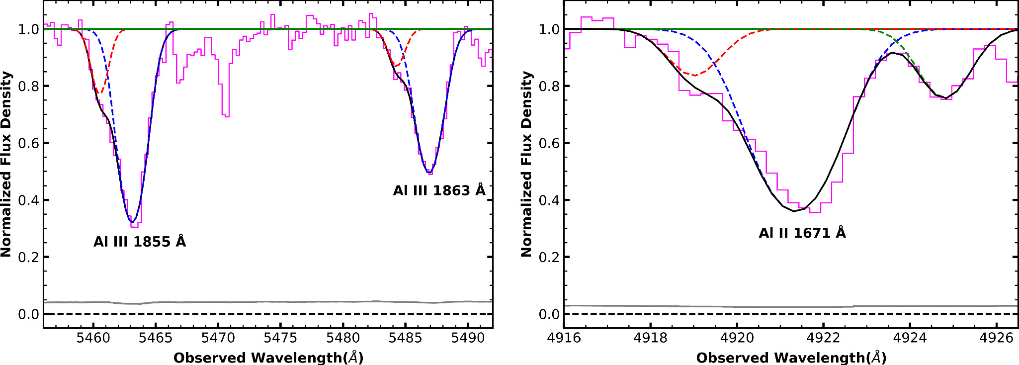
We model the troughs in velocity space using a Gaussian profile for the optical depth and note that for most of the observed ionic species (H i, N v, C ii, C iv, Si iii, and Si iv), the troughs appear saturated and therefore only lower limits for Nion can be obtained for them based on the AOD model. We detect troughs from two different ionized species of Al: Al iii λλ1855, 1863 and Al ii 1671 Å. We first model the Al iii 1863 Å trough with a Gaussian profile and then use this model as a template for the Al iii 1855 Å and Al ii 1671 Å troughs by fixing the centroid and width of the profile while allowing its depth to vary independently (see Appendix for an alternate multicomponent modeling and the difference between the two approaches). The best-fit models (shown in Figure 2) are determined by nonlinear least squares. We note that for Al ii, the deepest part of the model and the trough show a slight offset (∼30 km s−1). However, as this shift is less than one resolution element in the velocity space (∼73 km s−1), we continue to use this model for our analysis as it is physically motivated. As the two Al iii lines originate from the same lower energy level, we can use the PC method to obtain a measurement for the Nion. We find that the Nion determined using the PC method differs by less than 20% from the AOD determination, thus indicating that these troughs are not affected greatly by nonblack saturation. As the Al ii 1671 Å trough appears shallower than the Al iii 1855 Å trough, it would be affected even less by nonblack saturation (see Section 2.2 in N. Arav et al. 2018 for a detailed description of nonblack saturation). This allows us to use the Nion determined from the AOD method as a measurement. Reliable measurements of column densities from two different ionization states of Al play an important role in our photoionization analysis, which we describe in detail in the next section.

Figure 2. Detected troughs for the Al iii 1855 and 1863 Å (top) and Al ii 1671 Å (bottom) transitions along with their Gaussian models. The Gaussian models are based on the Al iii 1863 Å trough, and then its template with a fixed centroid and width is scaled to match the depth of the Al iii 1855 Å and the Al ii 1671 Å trough. The solid green line represents the local continuum model. The gray line shows the noise in the VLT/X-shooter flux.
Download figure:
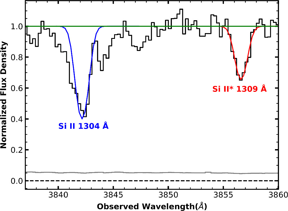
Standard image High-resolution imageFor Si ii, we detect multiple troughs originating from both the ground state and the 287 cm−1 metastable excited state. Among the detected Si ii transitions, the 1304 Å line has the smallest oscillator strength. It also appears much shallower than the other deeper Si ii troughs (at 1260 and 1527 Å) and can thus be considered unsaturated. Using the same argument to compare the different Si ii* transitions at 1265, 1309, and 1533 Å shows the 1309 Å trough can also be considered as unsaturated. Therefore, the AOD column densities derived from the Si ii/ii* 1304/1309 Å transitions can be used as measurements. Our modeling of these troughs follows the same procedure as that for the Al troughs. We first model the Si ii* 1309 Å trough with a Gaussian profile and use this as the template for obtaining the best-fit model for the Si ii 1304 Å trough (shown in Figure 3).

Figure 3. Observed troughs for the Si ii 1304 Å and Si ii* 1309 Å transitions along with their Gaussian models. The model is based on the Si ii* excited trough, and then its template with a fixed centroid and width is scaled to match the depth of the Si ii trough. The solid green line represents the local continuum model. The gray line shows the noise in the VLT/X-shooter flux.
Download figure:
Standard image High-resolution imageWe summarize the determined column density measurements and limits for the detected troughs in Table 2, along with the predictions of our best-fit photoionization model (Section 2.2.3). The reported errors include the uncertainty in determining the best-fit model for the unabsorbed emission. We first obtain the 1σ errors for the different components of our best-fit emission model (shown in red in Figure 1). Using them we construct two additional continuum models in which each component is shifted by +σ and −σ, respectively. We use these new continuum levels to renormalize the VLT/X-shooter spectrum individually and obtain the column densities of the different ionic species for them. Their deviation from the column densities obtained for the best-fit emission model (reported in Table 2) allows us to estimate their uncertainties due to our modeling of the emission features. We add them in quadrature with the 1σ uncertainties obtained similarly for our modeling of the absorption troughs. For Al ii, Al iii, and Si ii, we also include the uncertainty due to our choice of models for their troughs as outlined in Table 4 (see Appendix for a comparison between the single-component and multicomponent approaches).
Table 2. Ionic Column Densities for the Outflow in 3C 191
| Ion | log(Nion)a | log(N)b |
|---|---|---|
| (cm−2) | (cm−2) | |
| H i | 17.28 | |
| C ii | 15.21 | |
| C ii* | ⋯ | |
| C iv | 16.30 | |
| N v | 14.63 | |
| Al ii | 13.29 | |
| Al iii | 13.96 | |
| Si ii | 14.25 | |
| Si ii* | ⋯ | |
| Si iii | 15.46 | |
| Si iv | 15.56 | |
| S iv | 15.29 | |
| S iv* | ⋯ |


Notes. aMeasured column densities for the outflow from the VLT/X-shooter spectrum. bIonic column densities predicted by the best-fit Cloudy model shown by the black dot in Figure 4. The model values for C ii, Si ii, and S iv include the contribution from their excited states.
Download table as: ASCIITypeset image
2.2.3. Photoionization Modeling
Ionized outflows are dominated by photoionization equilibrium (K. Davidson & H. Netzer 1979; J. H. Krolik 1999; D. E. Osterbrock & G. J. Ferland 2006, and references therein) and are thus characterized by their total hydrogen column density (NH) and ionization parameter (UH), which is related to the rate of ionizing photons emitted by the source (QH) by

where R is the distance between the central emission source and the observed outflow component, c is the speed of light, and nH is the hydrogen number density. QH is determined by (a) the choice of spectral emission distribution (SED) that is incident on the outflow, (b) the observed flux of the object's continuum at a specified wavelength, (c) the redshift of the object, and (d) the choice of cosmology. Having determined the column densities of the observed ionic species, we can constrain the physical state of the gas, using the spectral synthesis code Cloudy (version C23.01; M. Chatzikos et al. 2023), which solves the equations of photoionization equilibrium in the outflow. The outflow is modeled as a plane-parallel slab with a constant nH and solar abundance, and is irradiated on by the modeled SED from the quasar HE0238-1904 (N. Arav et al. 2013), which is the best empirically determined SED in the extreme UV, where most of the ionizing photons come from. Figure 4 shows the result of our photoionization modeling. Using the methodology described by D. Edmonds et al. (2011), NH and UH are varied in steps of 0.1 dex, keeping all other parameters (nH, abundances, and the incident SED) constant, leading to a two-dimensional grid of models in the parameter space with predictions for all the Nion in the slab. The different-colored contours represent the allowed values in the (NH, UH) phase space that correspond to the observed column density constraints for the ionic species. The strongest such constraint comes from the column density measurements of the two Al ions. The ratio of the column densities of Al ii and Al iii serves as an indicator of the ionization state of the outflow that is independent of the assumed abundances. Therefore based only on the Al ii and Al iii Nion measurements, we obtain log NH = [cm−2] and log UH = . This solution is shown in Figure 4, surrounded by an error ellipse that contains the phase space values within one standard deviation of our best-fit solution. We use this solution for the rest of our analysis. As can be seen, this solution underpredicts the Si ii column density (traced by the blue curve). Furthermore, the constraint for Si ii is almost parallel to that for Al ii and therefore they cannot simultaneously be satisfied by any point in the (NH, UH) parameter space. The simplest way to resolve this conflict is to postulate an abundance ratio of Si to Al that differs from the one observed in the Sun. We find that an increase of ∼0.4 dex in the relative abundance Si/Al (with respect to the solar abundances) would ensure that the measured column density for Si ii matches our prediction from the model solution. Similarly, our model overpredicts the S iv column density (traced by the pink curve). However, the measurement can be brought in complete agreement with our model with a decrease of ∼0.35 dex in the relative abundance of S with respect to Al. The proposed changes for both Si/Al and S/Al abundance ratios are well within the ranges allowed by empirical abundance models in quasar outflows (N. Arav et al. 2013). Finally, Figure 4 shows that our model solution satisfies the lower limit constraints (represented by dashed curves) from all ionic species except N v. We note that N v has an IP of ∼98 eV and is thus associated with a region with higher ionization than the other observed ionic species in our analysis, which have IP ≲64 eV. Observations of quasar outflows in the extreme UV have shown that when reliable column densities for higher-ionization species (e.g., Ne viii and Mg x) can be obtained, a single ionization phase is unable to provide an acceptable physical model for the outflow, thus requiring two distinct ionization phases (N. Arav et al. 2013, 2020). The high-ionization species then correspond to a phase with higher NH and UH. From the VLT/X-shooter spectrum of 3C 191, we cannot obtain reliable measurements for the column densities of other high-ionization species, and therefore cannot constrain the high-ionization phase completely. However, N v can still be ascribed to this phase, and that would explain why its Nion constraint is not satisfied by our solution, which represents the low-ionization phase.


Figure 4. Plot of hydrogen column density () versus ionization parameter (), with constraints based on the measured ionic column densities. Measurements are shown as solid curves, while dashed curves show the lower limits, which allow the parameter space above them. The shaded regions denote the errors associated with each Nion as reported in Table 2. The phase space solution with minimized χ2 is shown as a black dot surrounded by a black ellipse indicating the 1σ error. This solution is based on the Nion of Al ii and Al iii (see Section 2.2.3). The black line marks the position of the hydrogen ionization front.


Download figure:
Standard image High-resolution image2.2.4. Electron Number Density
The ratios of the column densities of excited lines to those of the resonance lines are an indicator of the electron number density (ne) of an outflow under the assumption of collisional excitation (e.g., N. Arav et al. 2018). The identified outflow system in 3C 191 contains multiple troughs corresponding to the ground and excited states of Si ii. As discussed in Section 2.2.2, the Si ii 1304 Å and Si ii* 1309 Å transitions yield the most reliable measure of the column densities of Si ii and Si ii*. We obtain theoretical population ratios between the ground and excited states as a function of ne using the Chianti atomic database (version 9.0; K. Dere et al. 1997; K. P. Dere et al. 2019).
A comparison of these theoretical predictions with the observed ratio of column densities of Si ii* and Si ii is shown in Figure 5. This leads to log(ne) = [cm−3]. We also detect C ii 1335 Å and C ii* 1336 Å transitions, which appear to be saturated, and thus their AOD column densities will correspond to lower limits. Their ratio provides a lower limit of log(ne) [cm−3]. Although we do not detect the Si iv* 1073 Å trough, we use the Gaussian template obtained from the Si iv 1063 Å trough to obtain an upper limit for the column density of Si iv* based on its nondetection in the spectrum. The ratio of the Si iv* and Si iv column densities can then be used to determine an upper limit of log(ne) [cm−3]. Figure 5 shows that the obtained upper and lower limits are in agreement with our ne determined from the Si ii* and Si ii population ratio.


Figure 5. Dashed curves represent the theoretical population ratios for the transitions for an effective electron temperature Te = 8500 K (determined from our Cloudy modeling). The solid horizontal lines represent the observed column density ratios and their corresponding errors/limits.
Download figure:
Standard image High-resolution image2.3. Distance and Energetics
2.3.1. Distance Determination
Having determined UH and ne, we can use Equation (3) to obtain the distance between the outflow and the central source (R):

QH can be obtained by integrating over the SED for energies above the Rydberg limit:

The spectrum obtained from quasars with low-ionization absorption line outflows can be strongly affected by extinction due to dust in the host galaxy (P. B. Hall et al. 2002; J. P. Dunn et al. 2010; K. M. Leighly et al. 2024). To account for this reddening, we follow the methodology described by P. B. Hall et al. (2002), which includes dereddening the spectrum until the continuum slope matches that of the composite SDSS quasar of D. E. V. Berk et al. (2001). In doing so, we find that the slope of the composite SDSS quasar matches that of the HE0238 SED for frequencies smaller than that of the Lyα line. The HE0238 SED is thus representative of a typical dereddened quasar spectrum. Therefore, to obtain the dereddened SED incident on the cloud, we scale the HE0238 SED, by matching its flux to the observed flux from the VLT/X-shooter spectrum at an observed wavelength of λobs = 10000 Å (λrest = 3386.78 Å). We choose the longest available wavelength for scaling as AGN extinction curves show that the extinction generally increases with an increasing wavenumber, and is therefore smaller for longer wavelengths (B. Czerny et al. 2004; C. M. Gaskell et al. 2004). The resulting scaled SED is shown in blue in Figure 6. The ionizing photons come from wavelengths shorter than the Lyman limit, which is not covered by VLT/X-shooter. Therefore to get a handle on the ionizing continuum we use the available Chandra observations of the object covering the 0.2–2 keV range, obtained from the second release of the Chandra Source Catalog (I. N. Evans et al. 2010, 2020). The photometric flux measurements (converted to luminosity) are shown in the quasar rest frame in Figure 6 as red points. The X-ray measurements are in agreement with the prediction from the scaled HE0238 SED, further strengthening our case for its use to model the incident flux on the cloud. Therefore, based on our scaled SED, we obtain QH = × 1056 s−1 and bolometric luminosity LBol = × 1046 erg s−1.


Figure 6. SEDs considered in the analysis. The blue curve corresponds to the scaled HE0238 SED, with the VLT/X-shooter flux used for scaling (at λobs = 10000 Å) given by the blue dot. The orange curve shows the SED used by F. W. Hamann et al. (2001) and the black curve shows the Hamann SED rescaled based on the VLT/X-shooter flux (see Section 3.1 for more details). The red dots show the available X-ray flux measurements for the quasar. The errors on these measurements are between 5% and 15% and thus comparable to or smaller than the size of the points.
Download figure:
Standard image High-resolution imageTypically, nH is estimated from ne under the assumption of highly ionized plasma, which leads to the approximation ne ≈ 1.2nH. However, it has been shown that for the low-ionization phases of the outflow, the formation of the hydrogen ionization front can lead to a sudden drop in ne and therefore to an underestimation for nH (M. Sharma et al. 2025). We thus run a Cloudy model for our outflow with log(nH) = log(ne) = 2.78 and the parameters obtained in Section 2.2.3 and find that for this cloud, the hydrogen ionization front is not entirely developed, and thus while ne deviates slightly from the assumption of highly ionized plasma, the drop is not significant and averaging over the cloud based on the zonewise Si ii column density yields ne ≈ 1.1nH. Substituting the determined values of QH, UH, and nH into Equation (4), we find that the outflow is located kpc away from the central source.

To obtain an estimate of the systematic error in the distance determination due to different SEDs, we check the difference between the QH and UH determined from the HE0238 SED and the SED used by F. W. Hamann et al. (2001) in their Keck/HIRES analysis. The latter leads to a 25% increase in QH and a 7% decrease in UH. Therefore, using Equation (4), we can estimate the systematic error in our distance determination to be ∼16%.
2.3.2. Energetics
The outflow can be modeled as a partially thin spherical shell covering a solid angle Ω, and moving with velocity v (B. C. Borguet et al. 2012b). The total mass of the gas within the outflow can then be obtained as

where R is the spatial extent of the outflow, NH is the total hydrogen column density, mp is the proton mass, and μ = 1.4 is the atomic weight of the plasma per proton. Defining the dynamic timescale as the time it takes the gas from the nucleus traveling at an average velocity v to reach the location of the outflow, tdyn = R/v, we can obtain the mass-loss rate and the kinetic luminosity of the outflow as follows:


We assume Ω = 0.2 based on the ratio of quasars that show a C iv BAL (P. C. Hewett & C. B. Foltz 2003). Using the velocity at the deepest absorption (v = − km s−1) as the average velocity of the outflow leads to a mass-loss rate of = M⊙ yr−1 and kinetic luminosity = × 1042 erg s−1 for the outflow, which is × 10−3% of LBol. This is much smaller than the ≳0.5% required for efficient AGN feedback as determined by P. F. Hopkins & M. Elvis (2010).


3. Revisiting the Keck/HIRES Analysis of Hamann et al. (2001)
F. W. Hamann et al. (2001) observed 3C 191 using HIRES on the Keck I telescope on Maunakea, Hawaii. Using multiple observations adding up to 42,000 s, they covered the wavelength range λ ∼ 3530–8927 Å with spectral resolution R ≈ 45,000 and 3σ uncertainties ≲7% for the final fluxes. Using the emission line redshift of z = 1.956 determined by D. Tytler & X.-M. Fan (1992), they identified an outflow system covering a velocity range −1400 ≲ v ≲ −400 km s−1, with three components: −1400 ≲ Δv1 ≲ −1160 km s−1, −1160 ≲ Δv2 ≲ −810 km s−1, and −810 ≲ Δv3 ≲ −400 km s−1. If we instead use the redshift determined by Q. Zhao et al. (2025) (z = 1.9527), these components would have the velocities −1060 ≲ Δv1 ≲ −820 km s−1, −820 ≲ Δv2 ≲ −470 km s−1, and −470 ≲ Δv3 ≲ −60 km s−1. The outflow identified in the VLT/X-shooter spectrum (with −950 ≲ v ≲ −500 km s−1) is thus consistent with their system 2, which is their main outflow component, showing troughs from all species (see their Figure 2 and Table 1). We can see their system 1 and 3 in the blue and red wings, respectively, of our troughs, but our Gaussian modeling is able to isolate the main component (see Figures 2 and 3), thus allowing us to compare the results of their analysis with ours.
F. W. Hamann et al. (2001) analyzed the outflow in great detail and estimated its radial distance to be R ≈ 28 kpc from the central source. They determined log(U) ≈ −2.8 based on the comparison of the ratio of the Al ii/Al iii column densities to the theoretical ionization fractions in the optically thin photoionized cloud using Cloudy. They also utilized the ratio of Si ii 1527 Å and Si ii* 1533 Å to obtain an estimate of the electron number density ne ≈ 300 cm−3 and assumed nH = ne. Finally, they modeled the ionizing spectrum as a power law with Lν ∝ να, where α = −1.6 for frequencies above the Lyman limit, and α = −0.7 below it (the orange curve in Figure 6). Then they obtained the radial distance of the outflow using their Equation (6):

where α = −1.6, h is the Planck constant, and LLL is the luminosity density at the Lyman limit in the quasar rest frame, which was estimated by extrapolation of the data to the Lyman limit using the prescribed α = −0.7, with LLL ≈ 3.6 × 1031 erg s−1 Hz−1. This results in

where all the values are in cgs units. This leads to R ≈ 1.38 × 1023 cm = 44.6 kpc. This is 1.6 times larger than their reported value of R ≈ 28 kpc obtained using the same parameters. Both of these values are off by a factor of several when compared to the distance determined from our analysis of the VLT/X-shooter spectrum (R ≈ 5 kpc), and therefore we take a detailed look at this discrepancy in the following sections.
3.1. Change in Continuum and Extrapolation to Lyman Limit
We compare the SED used by F. W. Hamann et al. (2001) with the scaled HE0238 SED used in our analysis in Figure 6. This reveals that their νLν is roughly six times larger around the Lyman limit. To understand this difference, we compare the observed spectra obtained from both Keck/HIRES and VLT/X-shooter. At the longest available observed wavelength from their Figure 1, λobs ≃ 4976 Å, the measured flux density from the Keck/HIRES spectrum is Fλ ≃ 2.16 × 10⁻¹⁶ and that from the VLT/X-shooter spectrum is 0.91 × 10⁻¹⁶ [erg cm−2 s−1 Å−1]. A similar factor of increase in flux is also seen between the two spectra at λobs ≃ 4000 Å. Hence, while there is evidence for a change in continuum between these two epochs, it is much smaller than the difference seen in the SEDs. A likely reason for this could be the interpolation performed by F. W. Hamann et al. (2001) from their flux measurement at lower frequencies to the expected flux at the Lyman limit. The Keck/HIRES spectrum is limited on the short-wavelength end by λrest ≳ 1160 Å and therefore their interpolation to shorter wavelengths is based on their power-law index as discussed in the previous section. If we assume that the factor of increase in the continuum remains the same over the wavelength range, we can obtain an estimate for the Keck/HIRES flux at λobs = 10000 Å of Fλ ≃ 1.09 × 10⁻¹⁶ erg cm−2 s−1 Å−1. Using this to scale their SED gives us an estimate for LLL for the Keck/HIRES spectrum, with LLL ≈ 1.4 × 1031 erg s−1 Hz−1. This is roughly 40% of the estimate obtained by F. W. Hamann et al. (2001). The SED using the rescaled luminosity density is shown in Figure 6 in black.
3.2. Photoionization Modeling
Using the methodology described in Section 2.2.3 we can obtain a photoionization model of the outflow. F. W. Hamann et al. (2001) determined a covering factor Cf = 0.7 for weak and intermediate lines, which they applied to the Al troughs to obtain their true column densities. They reported the corrected total column densities for Al ii and Al iii integrated over all three velocity components, but we are interested primarily in their component 2, for which they did not report the corrections explicitly. However, we can note from their Figure 2 that the Al ii 1671 Å and Al iii 1863 Å troughs have similar residual intensities at their deepest point with Ir ≈ 0.25. Therefore any covering factor correction would affect them in the same way and would thus not significantly change their ratio, which is the indicator of the ionization state of the outflow. Therefore, we use their determined column densities of log(Nion) = 13.4 and 14.0 [cm−2] for Al ii 1671 Å and Al iii 1863 Å, respectively, for component 2, with an assumed error of ±0.1 dex based on the number of significant digits reported. We take the shape of the radiation incident on the cloud to be the same as the power-law SED of F. W. Hamann et al. (2001) and obtain the best-fit solution with log NH = [cm−2] and log UH = . This NH is roughly 1.7 times higher than our estimate from the VLT/X-shooter spectrum of log NH = [cm−2]. The UH based on their measurement is about 7% lower than our estimate of log UH = from the VLT spectrum, and is thus the same within the error bars. However, we note that this is ∼5 times larger than the U determined by F. W. Hamann et al. (2001), who found log(U) ≈ −2.8. We perform Cloudy simulations for an optically thin cloud and find that the ratio of Al ii and Al iii matches the observed ratio of column densities for log(U) = −2.8. However, we also find that the assumption of the cloud being optically thin does not hold throughout our model. The ionic fractions for Al ii and Al iii and their ratio for a Cloudy model with log NH = 20.72 [cm−2] and log UH = −2.09 are shown in Figure 7. We find that the optical depth at the Lyman continuum τLC becomes greater than 1 for NH ≳ 1020 cm−2 and the cloud is no longer optically thin. The ratio of the Al ii and Al iii ionic fractions therefore no longer remains constant, but instead increases as we approach the end of the cloud (the black curve in Figure 7). As most of the contribution to the Al ii and Al iii populations comes from these last zones, the average ratio for the cloud is significantly higher than that predicted by the assumption of the entire cloud being optically thin. Therefore the observed ratio of NAl ii/NAl iii ∼ 10−0.6 is reproduced by a cloud with ionization parameter log UH = −2.09. The cloud with ionization parameter log UH = −2.80 on the other hand predicts NAl ii/NAl iii ∼ 100.2, which is contradicted by the observations.


Figure 7. Ionic fraction within the cloud for log(UH) = −2.09. The blue and red curves show the ionic fractions of Al ii and Al iii, respectively, while the black curve shows their ratio.
Download figure:
Standard image High-resolution image3.3. Electron Number Density
F. W. Hamann et al. (2001) obtained the ratio of Si ii 1527 Å and Si ii* 1533 Å to get an estimate of the electron number density ne ≈ 300 cm−3, assuming a covering fraction Cf = 0.7. However we detect a much deeper Si ii 1260 Å trough in the VLT/X-shooter spectrum, which indicates a higher covering fraction for Si ii. At its deepest point, the Si ii 1260 Å trough has residual intensity Iv/I0 ∼ 0.1. Equation (2) from F. W. Hamann et al. (2001) would thus suggest Cf ≥ 0.9 for Si ii. Such high values of Cf would make a constant covering factor correction negligible for the Si ii troughs and therefore we consider Cf = 1. We also compare the Si ii 1527 Å and Si ii* 1533 Å troughs between the two epochs and find little variability for these troughs (see Figure 8). We note that the Si ii troughs seen in the Keck spectrum have a higher velocity than those seen in the VLT/X-shooter spectrum by ∼220 km s−1. The change in redshift from z = 1.956 to z = 1.9527 should result in a velocity shift of ∼340 km s−1. Therefore, if we use the same redshift, there is an offset of ∼120 km s−1 between the two spectra, which could be due to absolute wavelength calibration issues with the Keck spectrum.

Figure 8. Comparison between the Si ii 1527 Å trough obtained from the VLT/X-shooter spectrum (blue) and the Keck/HIRES spectrum (red). The Keck/HIRES spectrum was shifted in velocity space to match the troughs for this comparison. The green line shows the local continuum level, and the gray line shows the noise in the VLT/X-shooter flux.
Download figure:
Standard image High-resolution imageDue to the lack of any significant variation, we can use our column density measurements for these troughs as they are the same as F. W. Hamann et al. (2001)'s determination to the third significant digit, and allow for error estimation based on our modeling, with log(NSi ii) = [cm−2] and log(NSi II*) = [cm−2]. Following the steps described in Section 2.2.4, we match the ratio of the column densities to the theoretical prediction from Chianti and obtain ne = cm−3. This is in agreement with ne ≈ 510 cm−3 determined by F. W. Hamann et al. (2001) for Cf = 1. It is also in agreement with our determination of ne = cm−3 from the Si ii 1304 Å and Si ii* 1309 Å troughs in the VLT/X-shooter spectrum.


Finally, we run a Cloudy model for the outflow with the photoionization parameters obtained in Section 3.2 and find that the hydrogen ionization front is not entirely developed, similar to our finding from the analysis of the VLT/X-shooter spectrum. Thus we find that averaging over the cloud based on the zonewise Si ii column density again yields ne ≈ 1.1nH.
3.4. Distance Determination
We have determined some changes in the values obtained for LLL, U, and ne from the Keck/HIRES spectrum in our analysis so far in Section 3. Using these updated values with Equation (8), we find that the outflow is located kpc away from the central source. This distance is ∼79% smaller than the earlier determination of R ≈44.6 kpc based on the parameters reported in F. W. Hamann et al. (2001).

However, as we discussed in Section 2.3.1, the HE0238 SED is a better representative of the shape of the radiation incident on the cloud. Therefore we scale it to the expected Keck/HIRES flux at λobs = 10000 Å determined in Section 3.1. This leads to QH = 1.1 × 1057 s−1. We also use the HE0238 SED in the photoionization modeling with the Al column densities determined by F. W. Hamann et al. (2001) and find that it decreases the required ionization parameter to log UH = . Using these updated values with Equation (4) puts the outflow at a distance kpc away from the central source. This updated analysis brings the distance determined from the Keck/HIRES spectrum much closer to our estimate of kpc based on the VLT/X-shooter spectrum. The difference between these two distance estimates stems mostly from the difference in QH, which is due to the flux difference between the two spectra. If the Keck/HIRES spectrum is scaled to match the continuum level of the VLT/X-shooter spectrum, the distance of the outflow determined from the Keck/HIRES spectrum would be kpc, which is in good agreement with our distance determination from the VLT/X-shooter spectrum. We discuss the issues concerning this flux difference in Section 5.1.


4. Comparison with the IFS Analysis
3C 191 was also observed by the Spectrograph for Integral Field Observations in the Near Infrared (SINFONI) on VLT in multiple sessions between 2017 December and 2018 March (as part of program 097.B-0570(B), PI: Benn) with a total integration time of 4800 s. The observations covered a rest-frame spectral range of 4910–6266 Å, with spectral resolution of R = 3000, and angular resolution of , which corresponds to a spatial resolution of ∼2 × 2 kpc at the redshift of the quasar. In our companion paper (Q. Zhao et al. 2025) we analyze the ionized outflow in emission as traced by the [O iii] λλ4959, 5007 doublet. The [O iii] line profile is decomposed into three distinct velocity components: blueshifted, zero-velocity, and redshifted with respect to the quasar. The zero-velocity component is consistent with a typical narrow-line region for the quasar, while the blueshifted/redshifted components show strong signs of a bipolar outflow (see Section 4 of Q. Zhao et al. 2025, for a detailed description of the extended emission line features). For comparison with the outflow detected in absorption, we focus on the blueshifted component of the emission outflow.

The blueshifted outflow component seen in emission covers a velocity range −1090 ≲ v ≲ −20 km s−1. This is consistent with the outflow seen in absorption in the VLT/X-shooter spectrum spanning the velocity range −950 ≲ v ≲ −250 km s−1. This includes the main absorption system analyzed in this paper and its blue wing as seen in Figures 2 and 3. This kinematic correspondence between the outflows seen in absorption and emission suggests a common origin for them. Furthermore, the projected distance determined from the IFS mapping for the blueshifted outflow component is R ∼ 5 kpc (Figure 9). This is in remarkable agreement with the indirect distance determination of R = kpc obtained for the outflow based on the absorption analysis detailed in Section 2.3.1. This is the first instance where independent emission and absorption analyses of a quasar outflow have yielded consistent values for the distance of the outflow from the central source. While comparing the distances between our absorption and IFS analyses, it is important to note that they do not inherently measure the same distance. The absorption analysis measures the distance of the outflowing component from the central source along our line of sight, whereas the IFS analysis measures the projected distance in the sky plane. The relation between these two distances depends on the geometry of the outflow. Figure 9 (along with others in Q. Zhao et al. 2025) hints at a roughly spherically symmetric outflow, in which case the line-of-sight distance and the projected distance in the sky plane would be similar. However, other geometries for the outflow (such as a bipolar one) cannot be clearly ruled out on the basis of Figure 9 alone.


Figure 9. Median velocity map of the blueshifted component of the ionized outflow seen in emission. The red cross marks the position of the quasar and the smaller open circle depicts the point-spread function. The R = 5 kpc boundary centered around the quasar is shown by the bigger black circle.
Download figure:
Standard image High-resolution imageQ. Zhao et al. (2025) also estimate the energetics for the IFS manifestation of the outflow (see their Section 5.2 for a detailed description). The mass of the ionized gas is estimated using the [O iii] luminosity, using the ne determined from our absorption analysis. The mass-loss rate () and the kinetic luminosity () are then calculated accordingly, with the results summarized in Table 3. The energetics from the absorption analysis and the IFS analysis are consistent within a factor of 3, with the difference arising mostly from the smaller Mgas obtained for the IFS analysis. We note that the ionized gas masses obtained from the emission lines suffer from greater uncertainties than their absorption counterparts due to several factors, such as the temperature dependence of line emissivities. Moreover, as S. Carniani et al. (2015) show, the ionized gas mass traced by [O iii] is usually lower than that traced by Hβ, which was not covered in the observations analyzed by Q. Zhao et al. (2025).


Table 3. Kinematics and Energetics for the Outflow in 3C 191
| Parameter | Absorption Value | IFS Value |
|---|---|---|
| v (km s−1) | −950 to −500 | −1090 to −20 |
| R (kpc) | ||
| tdyn (yr) | × 106 | × 106 |
| Mgas (M⊙) | × 108 | × 107 |
| (M⊙ yr−1) | 9.5–13.4 | |
| Ekin (erg) | × 1057 | × 1056 |
| (erg s−1) | × 1042 | 2.6–3.7 × 1042 |


Notes. The reported values for the absorption analysis are only for the main component and do not include contribution from the associated absorption in the blue wing. For the IFS analysis, the reported kinematics are for the blueshifted component, whereas the energetics correspond to the blueshifted + redshifted components that make up the outflowing bubble.
Download table as: ASCIITypeset image
5. Discussion
5.1. Variability of the Central Source
As discussed in Section 3.4, the difference between the distance estimates obtained from the Keck/HIRES (1997 epoch) and the VLT/X-shooter (2013 epoch) analyses can be traced solely to a factor of ∼2.4 flux difference between the two spectra. During this period, 3C 191 was also observed by the Catalina Real-time Transient Survey (CRTS; A. Drake et al. 2009) between 2005 April and 2013 October. It was also observed later by the Zwicky Transient Facility (ZTF; E. C. Bellm et al. 2018; K. Malanchev et al. 2023) between 2018 March and 2023 February. Over the combined ∼15 yr of observation, the quasar showed little variability in flux (≲20%) in all the observed bands.
Moreover, Equation (3) suggests that variation in the ionizing flux should lead to a change in the ionization state of the gas given that the timescale of flux variation is comparable to the recombination timescale of the gas. For an absorber in photoionization equilibrium, if there is a sudden change of order unity in the incident ionizing flux, the timescale for the change in the ionic fraction of a species is given by (J. Krolik & G. Kriss 1996; N. Arav et al. 2012)

where ne is the electron number density of the gas, αi is the recombination rate of the ion i, and ni is the fraction of a given element in the ionization stage i. For the last zone of our modeled cloud, we can obtain ne, ni, and αi from Cloudy. The timescales for change in the ionic fractions of Si ii, Al ii, and Al iii can then be determined using Equation (10), resulting in ii ∼ 1 yr, ∼ 3 yr, and ∼ 31 yr. This suggests that a change in the ionizing flux from the quasar over a timescale t ≳ 1 yr would have led to a change in the observed troughs of Si ii and Al ii. However as shown in Figure 8, no significant change is seen in these troughs between the two epochs. This is consistent with the observations from CRTS and ZTF, and therefore the large difference in flux seen between the Keck/HIRES and VLT/X-shooter spectra is unlikely to be a result of intrinsic flux variation in the quasar. There could thus be possible issues with the absolute flux calibration for these observations.


5.2. Comparison with Other Outflows
G. Liu et al. (2015) obtained the IFS maps of two Seyfert 1.5 galaxies, IRAS F04250-5718 and Mrk 509, using the Gemini Multi-object Spectrograph (GMOS) on the Gemini South telescope (program ID: GS-2013B-Q-84; PI: D. Rupke). Both of these objects were already known to have shown outflows in absorption for which indirect distance constraints were available. G. Liu et al. (2015) detected ionized outflows in emission for both objects as traced by the [O iii] λλ4959, 5007 doublet, and thus presented one of the first such comparisons between AGN outflows analyzed using absorption and IFS techniques. Here we summarize the results of these analyses in brief.
IRAS F04250-5718. G. Liu et al. (2015) detected a biconical outflow extending out to ∼2.2 kpc on one side and to ∼2.9 kpc on the other. They determined the maximum line-of-sight velocity of the outflowing gas to be ∼330 ± 30 km s−1 based on modifications to the spherical outflow model of G. Liu et al. (2013), in which the opening angle of the outflow was measured to be ∼70° as per their IFS map of the [O iii] line width. Analysis of the outflow seen in absorption in this object was performed by D. Edmonds et al. (2011) based on high-resolution data obtained from the Cosmic Origins Spectrograph (COS) on the Hubble Space Telescope (HST). They identified three different kinematic components spanning the velocity range −290 ≲ v ≲ +30 km s−1. Based on the nondetection of excited states from C ii, they derived an upper limit on the electron number density of the outflow with ne ≲ 30 cm−3. This provided a constraint on the distance of the outflow from the central source and placed it at least 3 kpc away (R ≳ 3 kpc). This is consistent with the spatial extent of the outflow on one side of the quasar.
Mrk 509. The outflow detected from the IFS mapping by G. Liu et al. (2015) shows a roughly spherical morphology with a radius of ∼1.2 kpc, and velocity v ∼ 293 ± 51 km s−1. On the absorption front, S. Kraemer et al. (2003) obtained the Space Telescope Imaging Spectrograph (STIS) echelle spectrum of the AGN. Mrk 509 was also the subject of a large multiwavelength campaign (J. Kaastra et al. 2011), as part of which it was observed with HST/COS. G. Kriss et al. (2011) identified nine absorption systems spanning the velocity range −425 ≲ v ≲ +250 km s−1. Comparison between the C iv and N v troughs seen in the STIS and COS spectra showed negligible variation despite a large change in the ionizing flux. This allowed them to obtain upper limits on the electron number densities based on recombination timescale arguments. Using this, they determined a lower limit on the distance to the absorber of 100–200 pc from the ionizing source for all the components, which is again consistent with the spatial extent of the outflow determined from the IFS mapping (∼1.2 kpc).
Therefore, the IFS analysis of both of these objects reveals that the spatial extent of the outflows is consistent with the constraints determined from the indirect determination. However, as the absorption analysis only provides lower limits on the indirect distance determination, a conclusive correspondence cannot be drawn between the distances obtained from the two techniques. Therefore, a direct quantitative comparison of the absorption and emission techniques is featured for the first time in this work and our companion paper Q. Zhao et al. (2025).
6. Summary
This paper (along with the companion paper by Q. Zhao et al. 2025) presents a detailed study of the ionized outflow associated with the radio-loud quasar 3C 191 using absorption and IFS analysis techniques. In the VLT/X-shooter spectrum of the quasar, we identify an outflow system in absorption with velocity v ∼ −720 km s−1. We detect multiple ionized species covering a broad range of ionization and model the observed troughs to obtain their column densities (Section 2.2.2). We then obtain the best-fit photoionization model for the cloud with total hydrogen column density log NH = [cm−2] and ionization parameter log UH = based on the observed Al ii and Al iii column densities (Section 2.2.3). The detection of the metastable excited state of Si ii allows us to obtain the electron number density of the outflow with log ne = [cm−3] (Section 2.2.4). Combining these parameters with our informed assumption for the incident SED (Figure 6) locates the outflow at a distance of R = kpc from the central source. This leads to a mass-loss rate of = M⊙ yr−1 and kinetic luminosity = × 1042 erg s−1 for the outflow.


We note that our distance determination from the VLT/X-shooter spectrum is in disagreement with that of F. W. Hamann et al. (2001), who analyzed the Keck/HIRES spectrum of 3C 191 and placed the outflow at a much larger distance of R ∼ 28 kpc. We revisit their analysis in Section 3 and obtain different values for the number of ionizing photons (QH) and the ionization parameter (UH) based on our analysis techniques detailed in Sections 3.1 and 3.2, respectively. This leads to an updated value for the distance determined from the Keck/HIRES spectra of kpc, which is much closer to our estimate from the VLT/X-shooter spectrum.

Q. Zhao et al. (2025) detail our analysis of spatially resolved integral field observations of the ionized outflow surrounding 3C 191 obtained using VLT/SINFONI. In Section 4, we compare the properties of the [O iii] outflow seen in emission with those of the outflow detected in absorption. These two independent approaches lead to a remarkably consistent picture for the outflow as the distance determined indirectly using absorption analysis is verified by the spatial extent of the outflow determined directly from the IFS observations for the first time for a quasar outflow. The kinematics and energetics of the two manifestations of the outflow are also found to be in agreement as shown in Table 3.
Acknowledgments
We acknowledge support from NSF grant AST 2106249, as well as NASA STScI grants AR-15786, AR-16600, AR-16601, and AR-17556. Q.Z., L.S., and G.L. acknowledge support from the China Manned Space Project (the second-stage CSST science project: Investigation of small-scale structures in galaxies and forecasting of observations, Nos. CMS-CSST-2021-A06 and CMS-CSST-2021-A07), the National Natural Science Foundation of China (No. 12273036), the Ministry of Science and Technology of China (No. 2023YFA1608100), and the Cyrus Chun Ying Tang Foundations. Q.Z. and J.W. acknowledge National Natural Science Foundation of China (NSFC) grants 12033004 and 12333002. Q.Z. acknowledges support from the China Postdoctoral Science Foundation (2023M732955). We also thank the anonymous referee for constructive comments that helped improve this paper.
Appendix: Multiple-component Modeling of the Absorption Troughs
While determining the column densities for the outflowing system in Section 2.2.2, we model the troughs with a single Gaussian. However, as Figures 2 and 3 show, the absorption troughs of Al iii, Al ii, and Si ii show additional absorption in their wings. These components are not the focus of our analysis in this work as they do not show corresponding absorption for Si ii*. However, to ensure that they do not affect our column density measurement for the main component, we perform a multiple-component Gaussian fit for the entire absorption feature. We detail the fitting procedure for Al ii/iii and Si ii separately below.
A.1. Details of the Models
A.1.1. Al
We first model the Al iii 1863 Å trough with two independent Gaussian profiles for optical depth. We then use this model as a template for the Al iii 1855 Å and Al ii 1671 Å troughs by fixing the centroid and width of both Gaussians while allowing their depth to vary independently. In the case of Al ii 1671 Å, we allow for an additional component to model the absorption blend in the red wing. The results for the best-fit model templates (determined by nonlinear least squares) for these troughs are shown in Figure 10.

Figure 10. Multiple-component Gaussian modeling for the Al transitions. The main outflow component is shown as a blue dashed curve with the secondary component shown as a red dashed curve or as red and green dashed curves (for Al ii). The black solid curve shows the combined model for the troughs. The solid green line represents the local continuum model. The gray line shows the noise in the VLT/X-shooter flux.
Download figure:
Standard image High-resolution imageA.1.2. Si ii
The absorption trough for the Si ii* 1309 Å transition is well modeled by a single Gaussian component as shown in Figure 3. However the Si ii 1304 Å trough shows evidence for multiple components (four in particular, as can be noted by the two inflection points on the blue wing, and one more on the red wing). Therefore, we model the Si ii trough with four Gaussian components, of which one has a fixed centroid and width based on the Si ii* 1309 profile. The other three components are allowed to have centroids and widths that vary independently, and the depths of all the four components are allowed to vary as well. The results for the best-fit model templates (determined by nonlinear least squares) for these troughs are shown in Figure 11.

Figure 11. Multiple-component Gaussian modeling for the Si ii transitions. The main outflow component is shown as a blue dashed curve with the secondary components shown as red, green, and yellow dashed curves. The black solid curve shows the combined model for the troughs. The solid green line represents the local continuum model. The gray line shows the noise in the VLT/X-shooter flux.
Download figure:
Standard image High-resolution image
A.2. Change in Column Density
We now investigate the effect of the different models on the column density measurement for our main outflow component. To do so, we obtain the column density of the main component (shown in blue in Figures 10 and 11) from the multicomponent modeling and compare it with the column density obtained from the single Gaussian fitting shown in Figures 2 and 3. We report the percent change in the column density measurement due to the multiple-component approach in Table 4. The differences for all three ions are less than 5% and therefore we use the one-component Gaussian model for our analysis as it has fewer free parameters. We include this uncertainty due to our choice of models in the column densities reported in Table 2.
Table 4. Difference in Column Density Measurements Based on the Two Approaches
| Ion | ΔNion (%) |
|---|---|
| Al ii | −4.5 |
| Al iii | −4.5 |
| Si ii | −2.7 |
Download table as: ASCIITypeset image