


Abstract
Light–matter interactions lie at the heart of our exploration of exoplanetary atmospheres. Interpreting data obtained by remote sensing is enabled by meticulous, time- and resource-consuming work aiming at deepening our understanding of such interactions (i.e., opacity models). Recently, P. Niraula et al. pointed out that due primarily to limitations on our modeling of broadening and far-wing behaviors, opacity models needed a timely update for exoplanet exploration in the JWST era, and thus argued for a scalable approach. In this proof-of-concept study, we introduce an end-to-end solution from ab initio calculations to pressure broadening, and use a perturbation framework to address the need for precision to a level of ∼10%. We focus on the CO2–H2 system as CO2 is a key absorption feature for exoplanet research (primarily in many gas giants) at ∼4.3 μm as pressure-broadening parameters required for interpreting such observations remain sparse. We compute elastic and inelastic cross sections for the collisions of ortho-H2 with CO2, in the ground vibrational state, and at the coupled-channel fully converged level. For scattering energies above ∼20 cm−1, moderate precision intermolecular potentials are indistinguishable from high-precision ones in cross sections. Our calculations agree with the currently available measurements within 7%, i.e., well beyond the precision requirements.

Original content from this work may be used under the terms of the Creative Commons Attribution 4.0 licence. Any further distribution of this work must maintain attribution to the author(s) and the title of the work, journal citation and DOI.
1. Introduction
Among the JWST molecular observations, carbon dioxide is almost universally observed in exoplanetary atmospheres. From hot Jupiters such as WASP-39 b (P. Niraula et al. 2023; Z. Rustamkulov et al. 2023) to temperate sub-Neptunes such as K2-18 b (N. Madhusudhan et al. 2023), transmission spectra have shown the characteristic spectral feature at 4.3 μm. In fact, as this feature falls in a spectral sweet spot where the overall noise budget and the effect of cloud and/or hazes are minimal, it is also ideal for the detection of temperate terrestrial atmospheres and assessing their (in)habitability (e.g., A. H. M. J. Triaud et al. 2023; TRAPPIST-1 JWST Community Initiative et al. 2024).
Yet, despite these numerous favorable aspects, exploring exoplanet atmospheres using CO2 can be challenging due to the current state of its opacity model. P. Niraula et al. (2022, henceforth N22) pointed out that the current limitations of opacity models (primarily due to broadening and far-wing parameterizations) can yield an accuracy wall on the inferred atmospheric properties at the level of ∼1 dex, orders of magnitude above JWST’s capabilities (see Figure 1 for general framework). P. Niraula et al. (2023) subsequently highlighted that the aforementioned 4.3 μm feature of CO2, while dominant in most exoplanet spectra, can be challenging to translate into robust atmospheric inferences for a large range of exoplanets as these will harbor a hydrogen-dominated atmosphere, and very scarce data exist for broadening of CO2 lines by collisions with H2, especially at higher temperatures (R. Hanson & K. Whitty 2014; A. Padmanabhan et al. 2014). This is partly because the experiments on carbon dioxide and molecular hydrogen mixtures, especially at elevated temperatures, are very challenging from a safety perspective, adding extra complexity and expense to already existing difficulties in making accurate measurements of broadening parameters. Due to a lack of data, the HITRAN spectroscopic database (I. E. Gordon et al. 2022; Y. Tan et al. 2022), for instance, uses a very approximate solution of scaling the well-known air-broadening data based on limited hydrogen-broadening data. Since the dependence of air- and hydrogen-broadening data on the type of the transition is very different, the errors associated with this approach can be quite large.
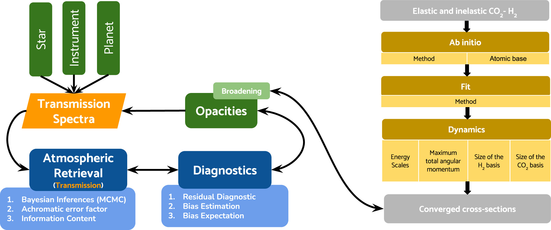
Figure 1. Flowchart for exoplanet atmosphere retrieval focusing on broadening parameters, as a key source of limitations in current opacity models (adapted from N22). Ab initio calculations are performed with the MOLPRO code (H.-J. Werner et al. 2015). Fits are done with Rist (C. Rist & A. Faure 2012) and YUMI for scattering and dynamics (N. Jaïdane et al. 2025, in preparation).
Download figure:
Standard image High-resolution imageIn the light of the hurdles in providing a solution to the opacity challenge on a timescale relevant to the JWST mission, this study presents the viability of a new-generation framework for ab initio calculations with a focus on pressure-broadening coefficients (typically defined as half-widths at half-maximum; I. E. Gordon et al. 2022). Different theoretical methods for calculating the pressure broadening employing classical dynamics/semiclassical quantizing exist, with various degrees of approximation (J.-M. Hartmann et al. 2018; N. H. Ngo et al. 2021). For example, J. Buldyreva et al. (2024) have used classical phase-shift theory to provide some data/estimates for the UV–visible range. There is also a large series of classical computations using very approximate potentials, but capable of computing the whole line shape, including the far wings (J.-M. Hartmann et al. 2002). Also, E. R. Guest et al. (2024) have investigated machine learning to provide broadening data based on HITRAN parameters. This is one avenue that would be considered state-of-the-art, but is limited by the learning set and will struggle to predict broadening for molecules/systems not included. In other words, while the ab initio calculation is not the only theoretical approach to address the opacity-driven accuracy wall (a wall which is expected to be hit once the retrieved precision surpasses 1 dex; see Figure 5 in N22), it is certainly one of the most accurate (see, for instance, M. Gancewski et al. 2021; E. A. Serov et al. 2021). And, as shown here, it can provide a cost-effective and thus scalable solution that can be deployed in a timescale relevant for ongoing missions such as JWST.
First, we assess the precision requirement on the pressure-broadening calculations given JWST’s capabilities in Section 2. Then, in Section 3, we describe our method for calculating the pressure-broadening parameters for CO2 + H2. Our results are presented in Section 4. We discuss implications (including scalability) and conclude in Section 5. The necessary background pertaining to the pressure-broadening calculations is included in the Appendix B based on the notations in Appendix A.
2. Precision Requirements
In this section, we aim to provide a more granular understanding of the pressure-broadening contribution to the uncertainty budget in exoplanet atmosphere analysis than N22 in order to set the precision requirement on the pressure-broadening calculations. Following the approach of D. Berardo et al. (2024) and B. V. Rackham & J. de Wit (2024), we require that the opacity perturbations contribute to the uncertainty budget on the atmospheric properties derived no more than the measurement itself, ensuring instrument-limited science.
To this end, we perform cross retrievals with perturbed cross sections on the two synthetic planetary systems following the framework introduced in N22—one super-Earth (1.1 R⊕, 1.1 M⊕, around a 0.1 R⊙ M dwarf star) and a warm Jupiter (1.0 RJup, 1.0 MJup, around a 0.55 R⊙ K dwarf star). We use pandexo (N. E. Batalha et al. 2017) to model instrumental precision using the same setup as in N22. As we focus here on the influence of perturbations on pressure-broadening coefficients to test the sensitivity of atmospheric inferences on that single parameter, we use a simpler synthetic atmosphere than in N22, considering only four molecular species (hydrogen, helium, carbon dioxide, and water). For the super-Earth scenario, we consider a high-metallicity Mixing Ratio (MR) H2O = 0.1, MR CO2 = 0.1) isothermal (T = 300 K) cloudless atmosphere, whereas for the warm-Jupiter scenario we consider a slightly hotter low-metallicity atmosphere (T = 400 K; MR H2O = 2 × 10⁻⁴, MR CO2 = 1 × 10⁻⁴).
To estimate the perturbation level leading to biases of amplitude equal to the 1σ confidence interval on atmospheric inference given by the instrumental precision, we generate an ensemble of perturbed cross sections (“CS”). Perturbations relate here to the underlying pressure-broadening parameters, and the series of cross sections used are denoted by CSxYYY where x is either m (for multiplied) or d (for divided) and 1.00 ≤ YYY ≤ 3.00, thereby referring to the scaling of the pressure-broadening parameters. This ensemble includes 15 relevant cross sections. The nominal cross section, CS1.00, was produced using the best available parameters from HITRAN database, generated by a prescription that included scaling of the air-broadening parameters. The remaining 14 cross section were perturbed accordingly: CSd3.00 (i.e., all the broadening parameters are one-third of those reported as nominal), CSd2.00, CSd1.50, CSd1.25, CSd1.10, CSd1.05, CSd1.01, CSm1.01, CSm1.05, CSm1.10, CSm1.25, CSm1.50, CSm2.00, and CSm3.00 (i.e., all the broadening parameters are 3 times those reported as nominal). As in N22, we use HITRAN (I. E. Gordon et al. 2022) and HITEMP (L. S. Rothman et al. 2010) for our opacity model inputs. We then performed the injection–retrieval tests, generating the synthetic spectra using the unperturbed cross section (CS1) and performing the retrieval with all cross sections. We ran our atmospheric models with emcee for a step size of 5000, ensuring our walkers are fully converged.
Figure 2 shows the typical results derived here for the warm-Jupiter scenario. As found in N22, even for large perturbations on the cross sections, a good fit to the data can be found (no structure in the residuals) owing to compensation by the atmospheric parameters in the associated dimensions of the inverse problem. It serves as a reminder that obtaining a good fit does not guarantee confidence in our inferences (and models). In fact, it further stresses the need for efforts such as this study to produce models of sufficient, independently tested fidelity to guarantee that the inferences will be reliable. Indeed, without such an independent test of the model fidelity or the capability to leverage the quality of the fit (or lack thereof) to assess it, one could reach inferences suffering unknowingly—a key takeaway from N22. These compensations translate into biased inferences up to ∼1 dex, for example, on the abundance of absorbers such as carbon dioxide and water (right panels of Figure 2). While both water and carbon dioxide showcase biases up to ∼1 dex, the statistical significance of the biases for water appears more prominent due to the narrower posterior probability distribution, which results from the higher information content associated with water (primarily due to the wider wavelength range associated with its absorption features).
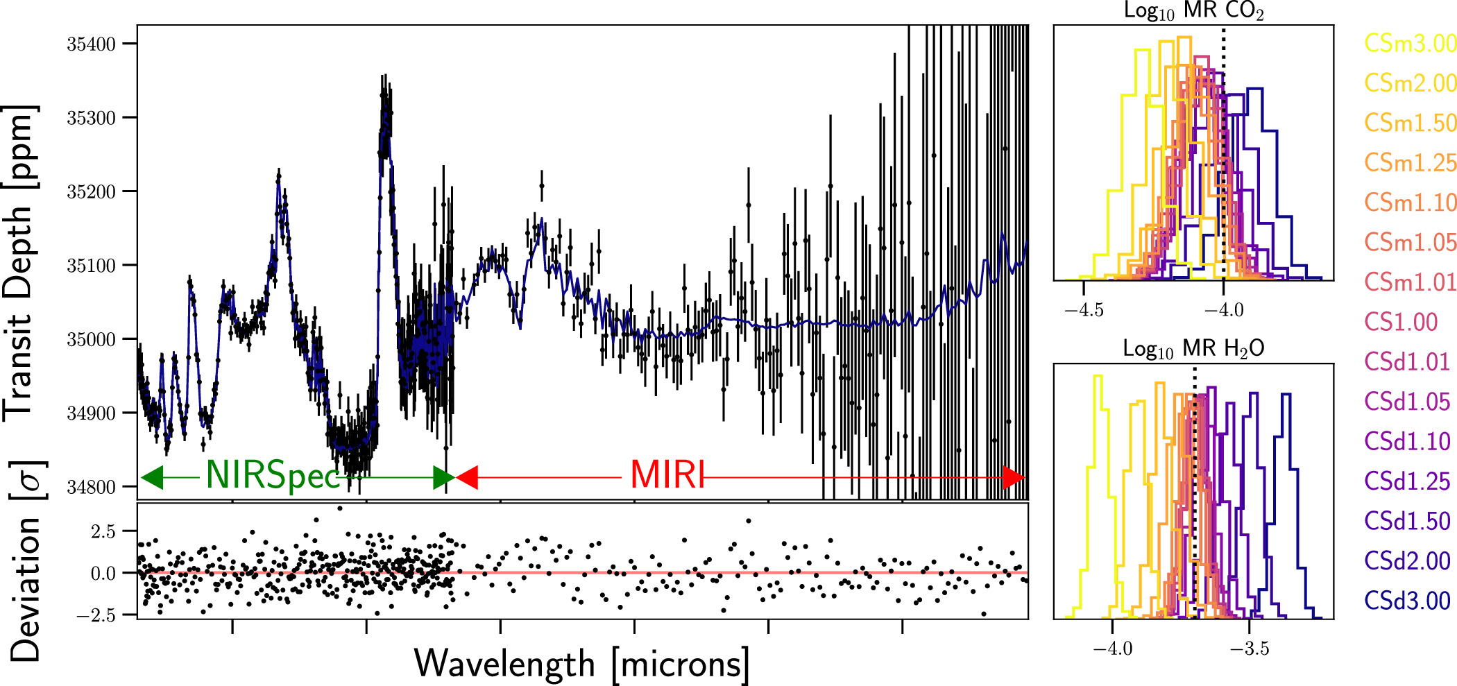
Figure 2. Perturbation analysis via injection–retrieval to assess the precision required on the broadening parameters in the JWST era. Top left: Synthetic transmission spectrum of a warm Jupiter spanning the NIRSpec and MIRI bands used for the retrieval. The blue line represents the best-fit model obtained when cross retrieved with the CSd3.00 cross sections. Bottom left: Deviation of the residual corresponding to the best fit presented on the upper panel. No structure is seen due to parameter compensation as highlighted in N22. Top right: Posterior probability distributions for the mixing ratio of CO2 for 15 different cross sections showing increased levels of bias with increased perturbation. The dotted black line represents the “truth” used for generating the synthetic spectrum. Overall variation of ∼1 dex is seen among the retrieved molecular abundance, consistent with N22. Bottom right: Same for H2O. A similar variation of ∼1 dex is seen overall, though leading to more significant biases due to the narrower distributions than for CO2.
Download figure:
Standard image High-resolution imageWe summarize our precision-requirement tests in Figure 3. As expected (and as shown in the right panels of Figure 2), it shows that the biases on the atmospheric inferences decrease with the perturbation level. The biases in Figure 3 are reported in significance level (σ), i.e., the ratio between the bias and the width of the distribution, which is solely driven by the measurement uncertainty. It shows that biases become marginal (i.e., below 1σ) when the perturbation on the broadening parameters drops below ∼10%. In other words, our precision requirement for broadening parameters to ensure instrument-limited science in the JWST era (i.e., avoid model-limited inferences) is 10% (see N22 for bias mechanisms; see P. Niraula et al. 2023 for their application to WASP-39 b).
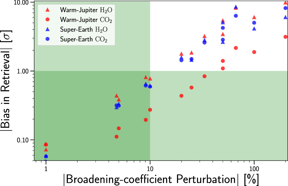
Figure 3. Greater than 5σ biases observed among the retrieved water and carbon dioxide abundances in our retrievals, with larger perturbations inducing stronger biases. The green region represents an acceptable bias range from −1σ to +1σ, demonstrating a need for a precision of 10%–15% in the pressure-broadening parameter for JWST observations.
Download figure:
Standard image High-resolution image3. Methods
With the well-justified precision requirement in hand, we can now turn to the series of calculations required to derive ab initio estimates of the broadening parameters. In this section, we provide an overview of the steps. For further details, refer to Appendix B.
3.1. Potential Energy Surface
We begin by computing the electronic interaction energy of the two molecules taken both as rigid rotors, employing the ab initio MOLPRO code (H.-J. Werner et al. 2015). We solve the electronic Schrödinger equation with fixed nuclei, using the quantum chemistry method CCSD(T), which allows for a good description of the electronic correlations, even for two molecules separated by a sizeable distance (here, up to 25 Å). The potential energy surface (PES) for the CO2–H2 interaction was computed for some 500 relative orientations of the molecules and for 29 intermolecular distances ranging from approximately 1.75 to 25 Å. For shorter distances, the two molecules repel so strongly (Einteraction ≳ 10,000 cm−1) that the approximation of two isolated molecules does not hold. For distances larger than about 25 Å, the interaction is weak (Einteraction ≲ 1 cm−1) and becomes neither reliable nor relevant for our computations. Note that because of the symmetry of both molecules (D∞h), the potential is π periodic in the dihedral angle ϕ and π/2 periodic in both polar angles θ1 and θ2 (see Figure B1).
We then fit the ab initio isolated points with a functional form according to the geometrical conventions of the angles ϕ, θ1, and θ2, see Equation (A9) of S. Green (1975) and Figure B1. We performed several fits of various precision, with 38 up to 158 terms, and found that an acceptable precision (∣Vfit − Vab initio∣/∣Vfit + Vab initio∣ ≤ a few %) is reached as soon as the orientation of the H2 molecules is described with at least l2 = 0, 2, 4 ) spherical harmonics. Ultimately, we used a 149 term expansion, up to l1 = 24 and l2 = 6 terms in
 ). 2D cuts of the PES are presented in Figure 4, emphasizing the change of the shape of the PES as the orientation of H2 changes.
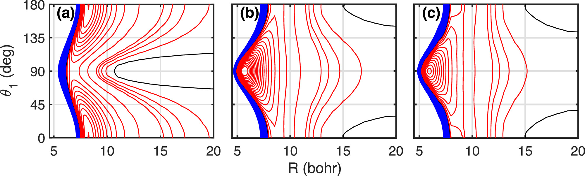
Figure 4. Three 2D cuts of the 4D interaction potential CO2–H2. Planar configurations: panel (a): θ2 = 0, ϕ = 0 and panel (b): θ2 = π/2, ϕ = 0. Nonplanar configuration: panel (c): θ2 = π/2, ϕ = π/2. Blue lines represent positive values of the potential, red lines show negative values, and the black lines represent zero values. Note that the potential is only asymptotically isotropic.
Download figure:
Standard image High-resolution image3.2. Dynamics: Broadening Coefficient
With the PES fits in hand, we can solve the quantum scattering dynamics in the time-independent domain, using the close-coupling (CC) formalism (S. Green 1975; P. Valiron et al. 2008). We use a home-written code (yumi), specifically designed for taking advantage of massively parallel computing. The code has been extensively tested against the existing state-of-the-art MOLSCAT code (J. M. Hutson & C. R. Le Sueur 2019), and will be described in detail in a forthcoming paper (N. Jaïdane et al. 2025, in preparation).
The quantum computations of the pressure-broadening cross section σPB(E) and the rate coefficient γ(T) are performed in the approximation of isolated binary collisions. It allows for no overlap between the different spectral lines; these hypotheses remain valid up to about one amagat of density (about 1019 particles cm–3) and for the P or R branches of the IR spectrum, but not for the Q branches. The isolated collision hypothesis allows for computing first the  matrices of the collision and derive from these the desired cross sections, whether elastic, inelastic, or pressure broadened, and the pressure shift (S. Green 1977; B. J. Drouin & L. Wiesenfeld 2012b; A. Faure et al. 2013; T. Selim et al. 2023). The cross sections are computed at given collision energies (the relative kinetic energy of the two molecules), then averaged over a Maxwellian distribution of kinetic energies to yield the relevant rates.
For this proof-of-concept application, we focus on reproducing the few experimentally known values, measured at different temperatures (R. Hanson & K. Whitty 2014; A. Padmanabhan et al. 2014), which connect an asymmetric stretch excited state with the ground state. The R. Hanson & K. Whitty (2014) measurement targets the P(24) transition of the 20012-00001 band, whereas A. Padmanabhan et al. (2014) cover the P(16)–P(34) transitions of the 30012-00001 band. (For spectroscopic notations, see Appendix A). Based on selection rules, the only allowed transitions are  . The nuclear spin statistics dictates that only even rotational levels in the ground vibrational state are populated because 12C16O2 is a symmetric molecule with zero nuclear spin values for all atoms, hence only even j1 in the ground state and odd j1 in the v3 = 1 case exist. The v1 excitation does not interfere with symmetry rules, being fully symmetric, merely acting as a spectator to the IR transition as demonstrated in experimental works (R. Hanson & K. Whitty 2014; A. Padmanabhan et al. 2014). For spectroscopic notations, see Appendix A.
The experimental values for the P24 (m = −24), in units of cm−1 atm–1, are γ = 0.112 (R. Hanson & K. Whitty 2014) and γ = 0.113 ± 0.006 (A. Padmanabhan et al. 2014), emphasizing the weak dependence on the exact vibrational transition. The errors bars from R. Hanson & K. Whitty (2014) are of the order of a few percent.
It has recently been shown (D. Yang et al. 2021; L. Wiesenfeld 2022) that computing inelastic scattering cross sections between two different rovibrational states is doable, but requires extremely large computational resources, which would render the scalability of our approach questionable. Fortunately, the pressure-broadening effect arises through quasi-elastic collision amplitudes, connecting the  or
 levels with themselves, but for different orbital angular momenta, see Appendix B.4. The experimental consequence is a very weak dependence of the pressure broadening on the molecular vibrations, except for some very anharmonic vibrations of modes containing atom(s) of hydrogen. The theoretical consequence is that we are allowed to consider the interaction potential and the dynamics as depending only on the average geometry of the molecules—rigid rotors approximation—and not on the vibrational dynamics, making the whole computation scalable. If selection rules allow (e.g., molecules of C∞h symmetry with no plane of symmetry perpendicular to the axis like CO or HCN), the pure rotational transitions serve as a proxy for the actual IR transitions (see, e.g., S. Green 1989; C. Luo et al. 2001; F. Dumouchel et al. 2010). For the case of molecules with D∞h (e.g., with a plane of symmetry perpendicular to the axis like CO2 or C2H2), the rotational selection rules differ from the vibrational selection rules. For CO2, only even rotational levels exist for the vibrational ground state and only odd rotational levels exist for the asymmetric stretch first excited levels (v3 = 1). We used these levels to compute pressure broadening for the P and R branches in the IR transition. Calculations by L. Rosenmann et al. (1988) show that there is practically no difference between the broadening of IR and Raman transitions of CO2 for several different projectile molecules, and they also did not observe vibrational dependence. (Note: “target” and “projectile” molecules are standard denominations in scattering studies, which respectively refer to the observed molecule—the target, and the bath molecule—the projectile, or broadener.) In general, when examining experimental data for linear molecules in the HITRAN database (R. Hashemi et al. 2020; I. E. Gordon et al. 2022; Y. Tan et al. 2022), weak or no dependence on vibrational modes is typically observed for linear molecules.
4. Results
As previously mentioned, our goal via this proof of concept of a scalable ab initio framework for broadening-parameter generation is to reproduce the only experimentally known values (R. Hanson & K. Whitty 2014; A. Padmanabhan et al. 2014), measured at different temperature.
The cross sections σ(Ecoll.; m = −24) (elastic, inelastic, and pressure broadening, see Appendix B) were computed for about 100 collision energies, ranging from 10 to 1500 cm−1. We present our findings in Figure 5, which shows that the precision requirements are achieved. For 296 K, the theory (γtheo = 0.120 cm−1 atm–1) slightly overshoots the experimental value (γexp. = 0.112 or 0.113 cm−1 atm–1). The difference (6.9%) is better than the precision requirement defined in Section 2. In R. Hanson & K. Whitty (2014), the temperature-dependent slope lacked error bars, and therefore should only be interpreted as an approximation.
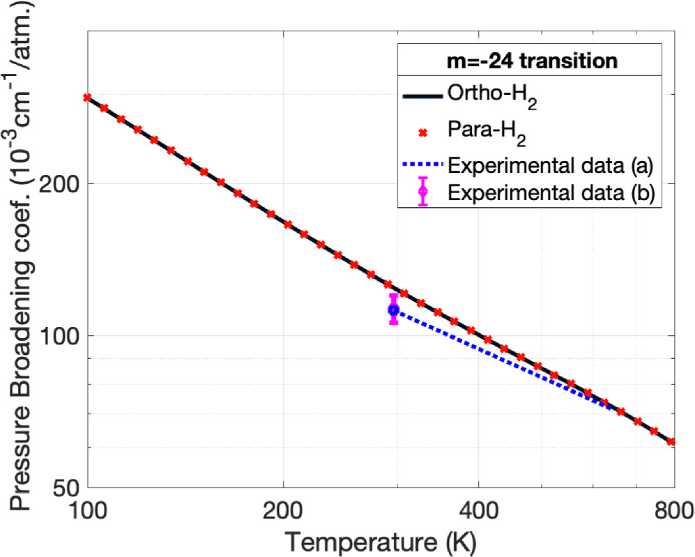
Figure 5. Theoretical pressure-broadening coefficient γ(T), for the m = −24 (P(24)) transition. The results for collisions with ortho-H2, j2 = 1 is shown in black, and those for para-H2, j2 = 0 in red. (a) Experimental data point and temperature dependence from R. Hanson & K. Whitty (2014); these experiments were performed from 300 to 640 K. (b) Experimental data point from A. Padmanabhan et al. (2014).
Download figure:
Standard image High-resolution image5. Discussion and Conclusion
5.1. Caveats and Previous State of the Art
Computations of the pressure-broadening coefficients for the aforementioned transition (i.e., m = −24) are performed through a series of codes that enables a full quantum dynamical approach to the problem, with no adjustable free parameters (see details in Appendix B). While the underlying theoretical framework was presented decades ago (e.g., M. Baranger 1958; S. Green 1977; G. Peach 1981), it is still able to provide accurate calculations today (J. M. Hutson & C. R. Le Sueur 2019; N. Jaïdane et al. 2025, in preparation). Indeed, while we assessed that a 10% precision of the line broadening parameters is required for state-of-the-art applications in exoplanetary sciences, we found that, for the transition computed, the agreement with existing measurements is well within this requirement (∼7%). While our calculations do not reach the accuracy achieved by the Torun group, who also compute non-Voigt parameters (e.g., M. Gancewski et al. 2021; E. A. Serov et al. 2021), our calculations are much faster (i.e., scalable) and can maintain a degree of accuracy required by atmospheric modeling applications.
Yet, a few remarks are in order. The calculated outputs for this particular transition (i.e., the m = −24 transition) exhibit only a weak dependence on any input parameter (except for the convergence of the quantum base, which remains paramount). For example, the σPB(E) function displays practically no structure nor dependence of the para or ortho character of H2. This is plausible due to particular aspects of the calculation. The occurrence of large quantum numbers included in the calculation significantly increases the number of channels (i.e., the quantum state during or after the collision), reduces quantum interference, and enables a semiclassical behavior of all the angular algebra (see J. Schaefer & L. Monchick 1987; Appendix B.4).
The complete ab initio computation of pressure-broadening coefficients has been undertaken, mostly with atomic colliders (F. Thibault et al. 2000; E. A. Serov et al. 2021; A. Godard Palluet et al. 2022) but also molecules (F. Thibault et al. 2011; L. Wiesenfeld & A. Faure 2013). All these ab initio calculations only require physical inputs for the experimental geometry of the target and projectile molecules and their experimental rotational constants, possibly from ground and vibrational excited states. The actual dynamics of vibrations (i.e., the full wave function of a rovibrator) has not been included in the dynamics as the vibrations play more of a spectator role, as underlined by the very small cross section that allows for vibrations to be excited or quenched (L. Wiesenfeld 2022).
5.2. Scalability
A fundamental advantage of the solution to the exoplanet opacity challenge presented here relates to its scalability. YUMI, our Fortran-based quantum scattering code, takes advantage of CPU architectures, in particular the extensive parallelism and memory hierarchies. The code has been optimized using an OpenMP framework, and streamlined for simultaneous multiple jobs submission leveraging tool kits such as LLTriple (C. Byun et al. 2015) developed for handling thousands of jobs in parallel. Our code performed at ∼30 GigaFlops during the speed benchmark test performed in an MIT SuperCloud node, which consists of an Intel(R) Xeon(R) Platinum 8260 CPU@2.40 GHz with 48 cores. The current speed bottleneck is the matrix inversion required for solving the Schrödinger equation (N. Jaïdane et al. 2025, in preparation; see also Appendix B), which involves a recursive algorithm implemented from C. Ingemarsson & O. Gustafsson (2015), built on top of Intel’s MKL library. Our algorithm scales at O(N∼2.6), i.e., smaller than three, with N, the matrix size. For CO2–H2, the typical matrix size is ∼1000, and the typical calculation takes less than ∼1 hr for a single transition at a particular energy. For a single transition, such calculations needs to be performed roughly at 100 different energies, and for more complex molecules such as water, matrix sizes reach ∼10,000. The related calculations would thus take ∼400 times more computational time (i.e., ∼2 weeks), significantly longer but still within our computational reach. Leveraging the symmetry within the molecule, GPUs, and possibly machine learning techniques in future applications will further help us enhance the scalability of our approach.
5.3. Future Prospects
The results presented in this study provide a proof of concept for a scalable solution to a key limitation behind the exoplanet opacity challenge, namely the modeling of broadening. While our application focuses on the data-scarce CO2–H2 collisional system due to its importance in most of the exoplanet spectra acquired with JWST and the scarcity of data available for the system, it can now be applied to the hundreds of other collisional systems of relevance for JWST and future missions.
While the CO2–H2 system could be investigated with sufficient funding and careful experimental works on an adequate timescale (∼1 yr), it is just one collisional system out of thousands of molecules of relevance. Unfortunately, measurements of broadening parameters with sufficient accuracy are challenging to make, and often rendered impractically complex and expensive due to safety issues (as a reminder, the primary targets of exoplanetary sciences remain hydrogen-rich high-temperature worlds). Therefore, the methodology presented here provides a timely and realistic approach to fulfilling the opacity needs of the exoplanet community, and helps pave the way toward robust atmospheric inferences reaching accuracy driven by the instrument itself (rather than opacity models).
Acknowledgments
J.d.W. and L.W. thank the MIT Global Seed Funds and MIT-France for their support toward this study. N.J. thanks Université Paris-Saclay for a visiting fellowship. I.G. and R.H. acknowledge NASA PDAR grant 80NSSC24K0080. L.W. and N.J. thank Olivier Dulieu for fruitful discussions. L.W., P.N., and J.d.W. thank Jeremy Kepner, Deborah Woods, and Cooper Loughlin for insights regarding optimal deployment on supercomputers, scalability, etc., which will be pivotal in the next steps of this project. Part of these computations were performed on the Jean-Zay IDRIS-CNRS supercomputer, contract A0140810769. Other parts were computed on the MIT SuperCloud/Lincoln-MIT computers. The authors acknowledge IDRIS and the MIT SuperCloud and Lincoln Laboratory Supercomputing Center for providing resources (HPC, software expertise, database, and consultation) that have contributed to the research results reported here.
Software: emcee (D. Foreman-Mackey et al. 2013), MOLPRO (H.-J. Werner et al. 2015), Matlab, tierra (N22), YUMI (N. Jaïdane et al. 2025, in preparation).
Appendix A: Notations
We used in this work the following conventions and notations:
Quantum numbers and spectroscopy. To avoid any ambiguity between commonly used notation for angular momenta, we use the following notation: j1 and j2, the angular momentum with respect to the CO2 and H2 molecule, respectively; l, the orbital angular momentum of the collision; and J, the total angular momentum of the collision (a conserved quantity for a collision). The running index m is defined as  for the P branch,
 for the Q branch, and
 for the R branch. Therefore for the transition studied here, m = −24 corresponds to P(24). Primed and double primed quantities are lower and and upper levels, respectively. If one looks at the HITRAN file for carbon dioxide they will see branch designation and the
 value for unique identification.
Vibrational levels of CO2 are given (in HITRAN notation) by [v1, v2, l2, v3, q], where vi are the three normal modes, i.e., symmetric stretch, bend, and asymmetric stretch, l2 is the rotational vibration quantum number, and q labels the levels of the same polyad.
Energy. Energies are defined as follows: (i) E is the total energy of the collision and (ii) the collision energy Ecoll. = E − Erotation(CO2) − Erotation(H2).
Appendix B: Quantum Dynamics
Our aim is to compute pressure-broadening coefficients for the 4.3 μm transition of 12C16O2; that is, the IR lines that correspond to  , broadened by collisions with H2. We aim at a full quantum ab initio scheme, based on the CC formalism (J. M. Blatt & L. C. Biedenharn 1952; M. Baranger 1958; A. M. Arthurs & A. Dalgarno 1960). In order to do so, one needs successively: (i) a series of ab initio potential energy points V(Rn) describing the interaction of CO2 with H2 (R, the four coordinates setting the geometry of CO2 with respect to H2); (ii) a fit of these V(Rn) points into a suitable functional form; (iii) solving the quantum dynamical equation of the collision, in order to get the S matrix connecting the entrance and outgoing channels of the collision (usually, solving the Schrödinger equation); and (iv) from knowledge of the S matrix, constructing the pressure-broadening cross sections and rate coefficients. This section describes the details of all four steps.
B.1. Potential Energy Ab Initio Points
We compute the pressure broadening by H2 of IR transitions of CO2. Hence, it would seem sensible to allow for CO2 vibrational modes to be included in the PES. However, vibrational motion influences very weakly the pressure-broadening coefficients (I. E. Gordon et al. 2022; Y. Tan et al. 2022), at least in the temperature regimes that we aim at, 50 ≤ T ≤ 1000 K. Note that the same does not seem to be true for line shifts. We thus restrain our computations to rigid body interaction. We use the ground state vibrational averaged geometries for CO2 and H2, with r(CO) = 2.1944 bohr (A. Godard Palluet et al. 2022) and r(HH) = 1.44836 bohr (E. Sahnoun et al. 2020). The PES has four degrees of freedom, namely, R, the distance between the center of masses of the two molecules, the θ1 and θ2 angles that describe the orientation of the two linear molecules with the intermolecular axis, and ϕ, the dihedral angle, see Figure B1.
In the vibrational ground state, both molecules display D∞h symmetry; the ground state intermolecular PES must reflect these symmetries. With the geometry defined in Figure B1, the whole PES is described by 0 ≤ θ1 < π, 0 ≤ θ2 < π/2, and 0 ≤ ϕ < π/2.
As the atoms are relatively light, and as we have to deal with 22 electrons only (among those, six core electrons), it is possible to compute the PES in multiple ways, of various precision. This allows us to study the influence of the PES precision on the observables, elastic and inelastic cross sections, and pressure-broadening rate coefficients in particular.
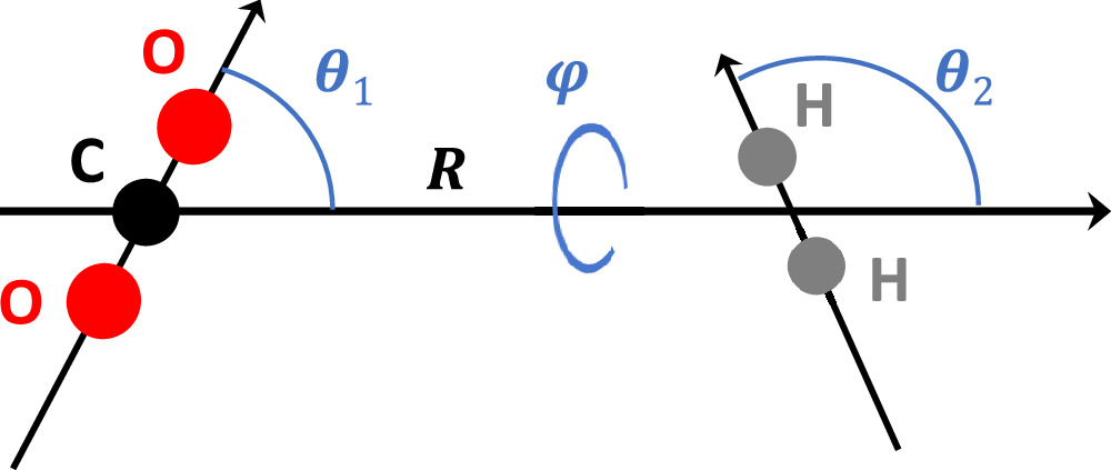
Figure B1. The four degrees of freedom (R, θ1, θ2, ϕ) of the CO2–H2 complex, in the rigid body approximation.
Download figure:
Standard image High-resolution imageB.1.1. Ab Initio Quantum Chemical Computations
The interaction energy is computed via the supermolecule approach, including systematically the basis set superposition errors (M. Kodrycka & K. Patkowski 2019; see also our previous works E. Sahnoun et al. 2018; M. Ben Khalifa et al. 2019 for a detailed description). All computations are performed at the CCSD(T) level, with the 2020 version of the MOLPRO code H.-J. Werner et al. (2015). The interaction energy is defined as:

were the superscript AB denotes the full molecular basis A ⊕ B, A ≡ CO2, and B ≡ H2.
In order to evaluate the precision needed for computing the elastic and inelastic cross sections of the collision CO2–H2, we used four precision levels for computing the interaction, all described in the documentation of molpro, (H.-J. Werner et al. 2015): (1) basis set aug-cc-pVTZ (denoted in the following as avtz), alongside with a bonding function center (R. A. Shaw & J. G. Hill 2018) at two-thirds of the distance between the center of mass of H2 and the nearest atom of the CO2 molecule (the PES depends very weakly to the actual position of the bonding function, as long as it is not too nearby any actual atom); (2) the same formalism but with the basis set aug-cc-pVQZ (denoted in the following by avqz); and (3) an extrapolation to the complete basis set, with the avtz and avqz values at each ab initio point, and the extrapolation formula (A. J. C. Varandas 2021):

The ab initio PES obtained via Equation (B2) is called hereafter avcbs.
The last formalism (4) is the so-called “gold standard,” widely used for computing intermolecular interactions: the CCSD(T)-F12a formalism (M. Kodrycka & K. Patkowski 2019). We used exclusively the avqz basis for this computation (even if avtz could yield very similar results). Using a bonding function proved unreliable and was not used. We noted the well-known problem of size inconsistency of the explicitly correlated F12 family of methods. We duly subtracted the value of the interaction at infinity (here, 50 bohr), which was isotropic within less than 1%.
Some points (see below) were computed at the aug-cc-pV5Z level (av5z), in order to have some hints of the convergence of the PES, on the one hand, and to see if the CCSD(T)-F12 methods are reliable, especially so for overshooting the minimum of the PES. Results around the different stationary points are shown in Table B1. As briefly explained beforehand, convergence at the wavenumber scale is essentially achieved for av5z and the more economical avcbs. The avqz method with the F12 acceleration slightly overshoots the values, and the avtz method is clearly less precise. However, all methods agree one with another within 4%–5% and with the earlier computations of H. Li et al. (2010).
Table B1. Minimum Vmin of the CO2–H2 Potential Energy Surface, at Intermolecular Distance Rmin
| Method | avtz | avqz | av5z | avcbs | avqz-F12 | H. Li et al. (2010) |
|---|---|---|---|---|---|---|
| Rmin (bohr) | 5.63 | 5.605 | 5.5875 | 5.595 | 5.585 | 5.612 |
| Vmin (cm−1) | −215.5 | −219.59 | −221.97 | −222.65 | −224.77 | −219.65 |
Note. The geometry is always θ1 = 90∘, θ2 = 90∘, and ϕ = 0∘. The partial av5z computations are included. Note that our computations are for average ground state geometries and those of H. Li et al. (2010) are for equilibrium geometries.
Download table as: ASCIITypeset image
B.2. Geometries and Fit
While some formalism allows for computing the PES with a limited number of points (M. Ben Khalifa et al. 2020; Y. Ajili et al. 2022), we decided to compute the PES on a dense grid of ab initio points, like we did repeatedly in previous cases, like E. Sahnoun et al. (2020), P. Valiron et al. (2008), C. Rist & A. Faure (2012), and M. Ben Khalifa et al. (2020). To summarize, we compute ab initio points for 500 sets of angles  per distance R. These angles are randomly chosen with 0 ≤ θ1,2 < π and 0 ≤ ϕ < 2π. In doing so, we do not impose the C∞h symmetries of H2 and CO2. The subsequent fit of the potential should reveal the symmetries (see below). We computed the potential for 29 distances, between 4.20 bohr and 50.00 bohr. Note that the random set of angles is the same for each distance, facilitating the fit.
We fit the PES distance by distance, with the following formula adapted from S. Green (1975):

with the angular function X equal to:
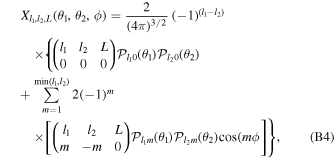
with (l1 + l2 + L) even and  are Wigner 3-j symbols. The normalization is:

We took great care to have the same expansions and normalizations of the angular functions  in this expansion and in the scattering code. To avoid any confusion, the explicit relations between the
 functions, the associated Legendre functions, and the spherical harmonics are given in R. N. Zare (1988), Section 1.3.
We tried three bases for the fit, indexed by the the maximum allowed values of the l1, l2, and L indices in Equation (B3), the so-called:
- (i)precise expansion, with l1 ≤ 24, l2 ≤ 6, and L ≤ 26, resulting in 158 terms in the expansion (B3); because of limited relevance, not all terms allowed by angular algebra are included;
- (ii)intermediate expansion, with l1 ≤ 20, l2 ≤ 4, and L ≤ 22, resulting in 76 terms; and
- (iii)imprecise expansion with l1 ≤ 20, l2 ≤ 2, and L ≤ 22, resulting in 38 terms.
In all cases, only even values of angular momenta are allowed, because of the symmetries of the molecules.
B.2.1. Potential Surface
We computed all 12 combinations {basis set} × {fit precision}, even if some combinations make little sense. For the precise fit, comparison of some stationary points of the V(R, θ1, θ2, ϕ) potential functions are given in Table B1. Figure B2 depicts the errors in the fit for the three levels.
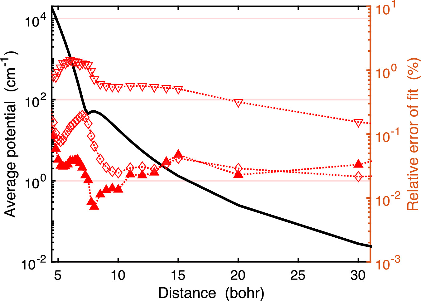
Figure B2. Different fits of the ab initio potential. The angle averaged absolute value potential is given by the thick black line. Relative fit errors are in red, with the scale on the right. The precise fit is shown with filled upper triangles; the intermediate fit with open diamonds; and the imprecise fit with empty lower triangles.
Download figure:
Standard image High-resolution imageB.3. Dynamics
In order to solve for the S matrix characterizing the scattering, we resorted to the well-documented time-independent CC formalism (see, e.g., A. M. Arthurs & A. Dalgarno 1960; J. M. Hutson & C. R. Le Sueur 2019; M. H. Alexander et al. 2023). In order to accelerate the computations and take advantage of the large memory available for each computing node in the high performance computers, we used a new home-written CC code. The main differences between the widely available MOLSCAT code and the present one are the native use of OpenMP capabilities—readily extensible to GPU-based OpenACC capabilities,5 as well as memory management capable of taking full advantage of the hierarchy of RAM in the cores and the nodes. A full description of the code will be available in a future publication.
B.3.1. Cross Sections
Once S or T matrices are available, it is simple to sum up all relevant contributions and get the elastic/inelastic cross sections at a given collision energy, σij(Ecoll), with i ≷ j. These computations are much more sensitive to the details of the PES than their pressure-broadening counterparts, as the next section will show. An example of the sensitivity to PES precision is given in Figure B3.
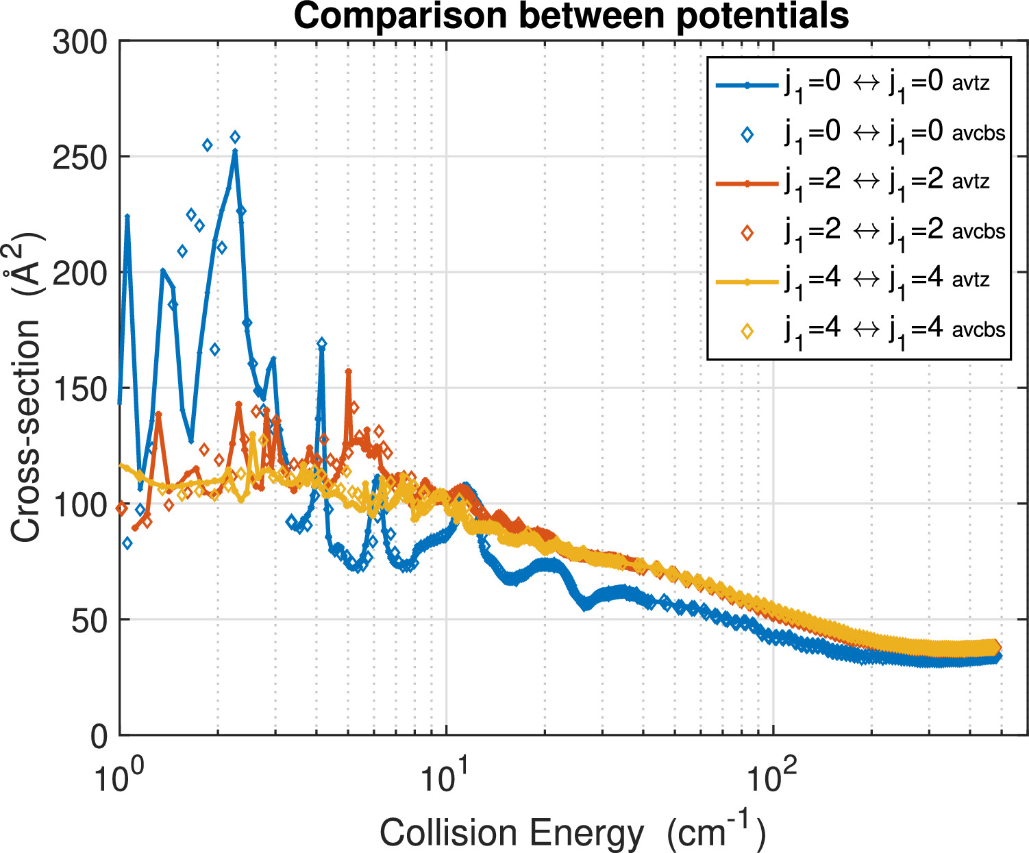
Figure B3. Comparison between two ab initio bases: the less precise (avtz basis, continuous line) and the most precise (avcbs, diamonds). Large fit was done, with 156 terms. Elastic cross sections are shown for the collision CO2–ortho-H2, where j1 is the CO2 rotational quantum number and v3 = 0.
Download figure:
Standard image High-resolution imageB.4. Pressure-broadening Computation
Knowledge of the S or T matrices allows for computing the collision-energy-dependent pressure broadening  . The formalism dates from M. Baranger (1958) and J. Schaefer & L. Monchick (1987).
The full analytical formula, Equation (1) of J. Schaefer & L. Monchick (1987) was used in order to compute σPB(Ecoll), for the transition  , at about 100 different collision energies Ecoll. The degeneracy factor
 was taken into account, see remarks in S. Green (1975) and L. Wiesenfeld & A. Faure (2013). At each energy, four events were computed: collision with H2, j2 = 0,
 or 25, and the same with H2, j2 = 1. Results are presented Figure B4. The remarkable smoothness of the results contrasts with the multiple resonances observed in elastic cross sections, like Figure B3.
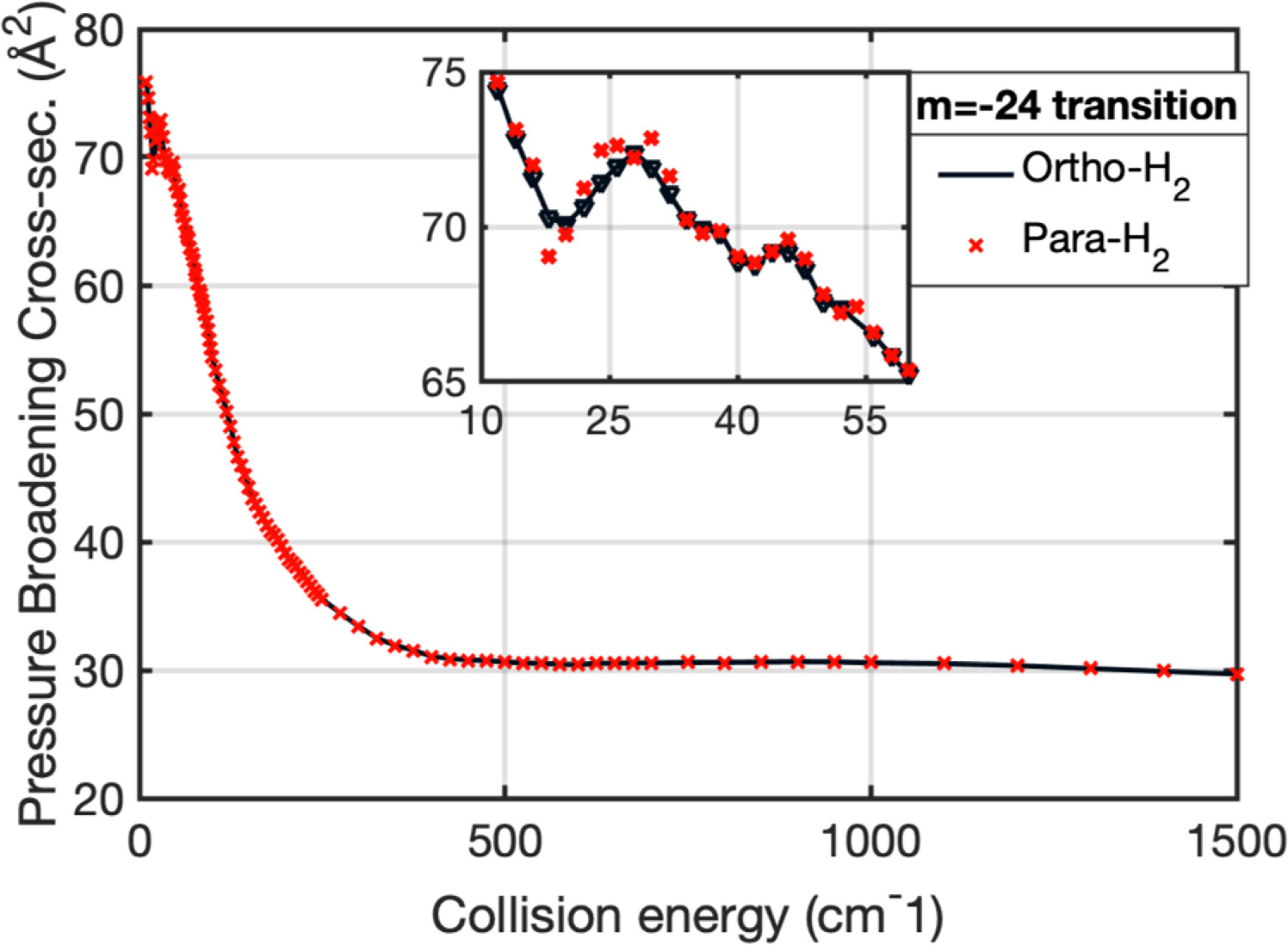
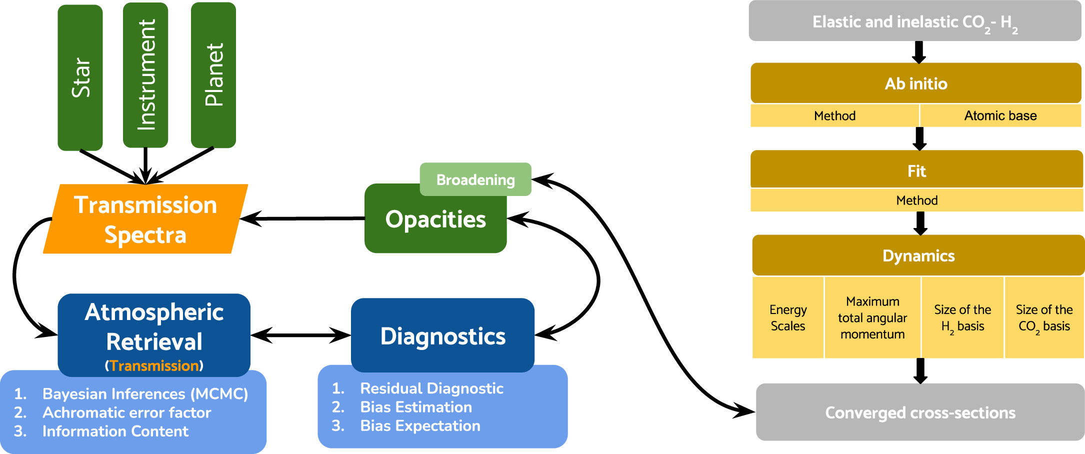
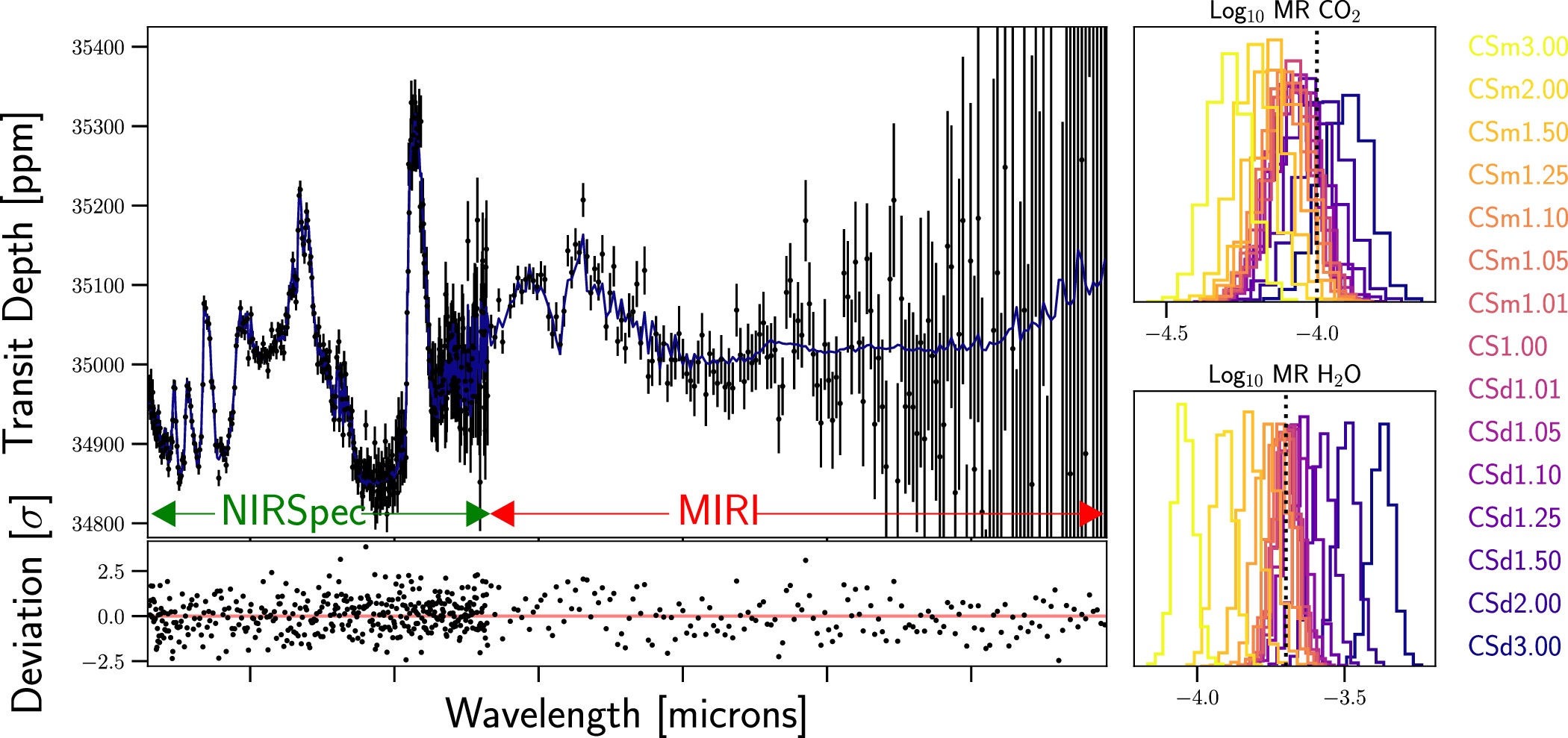
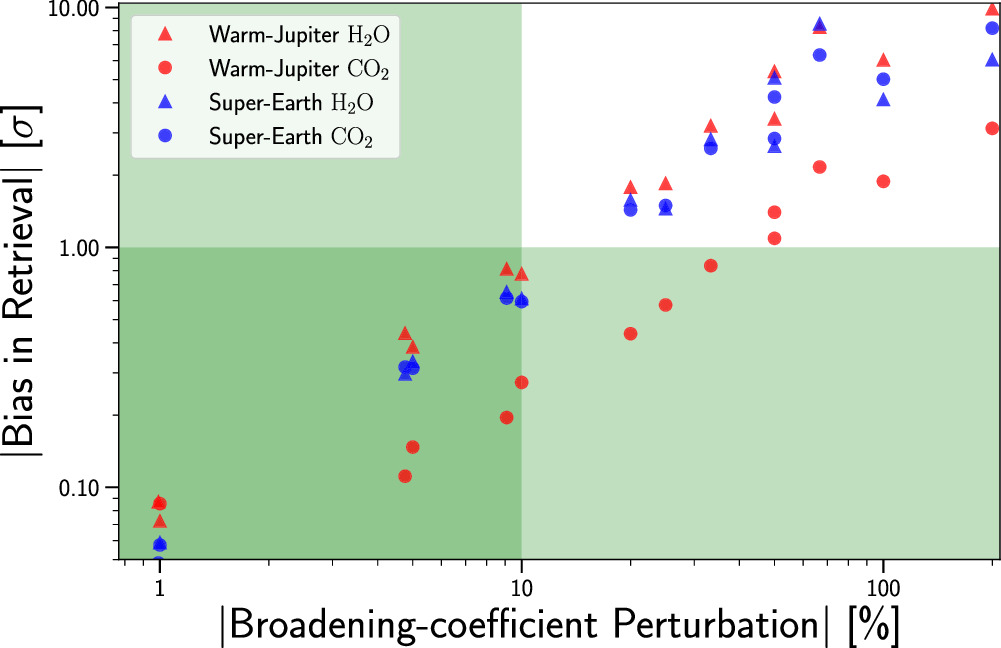
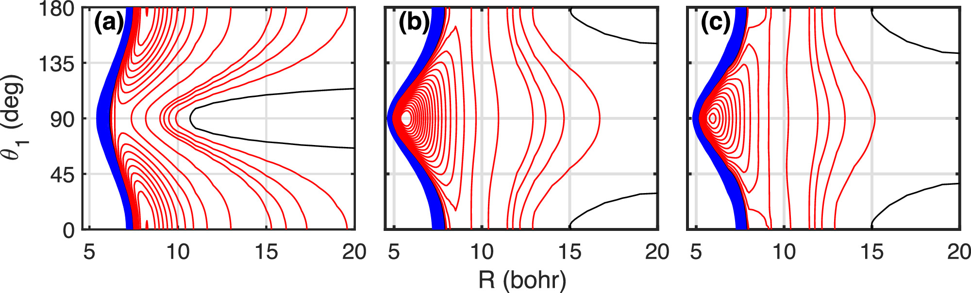
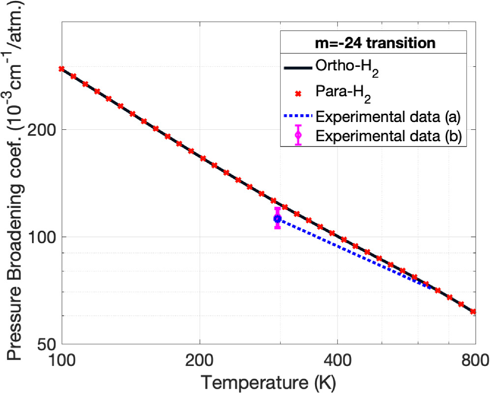
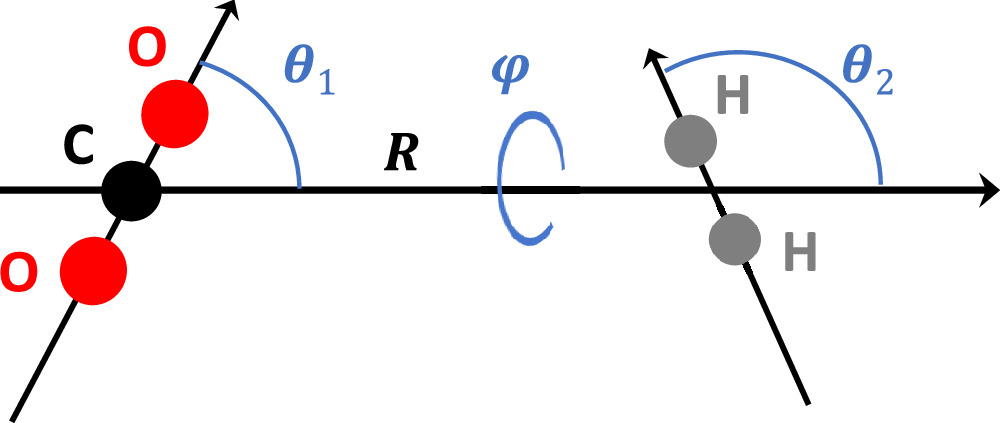
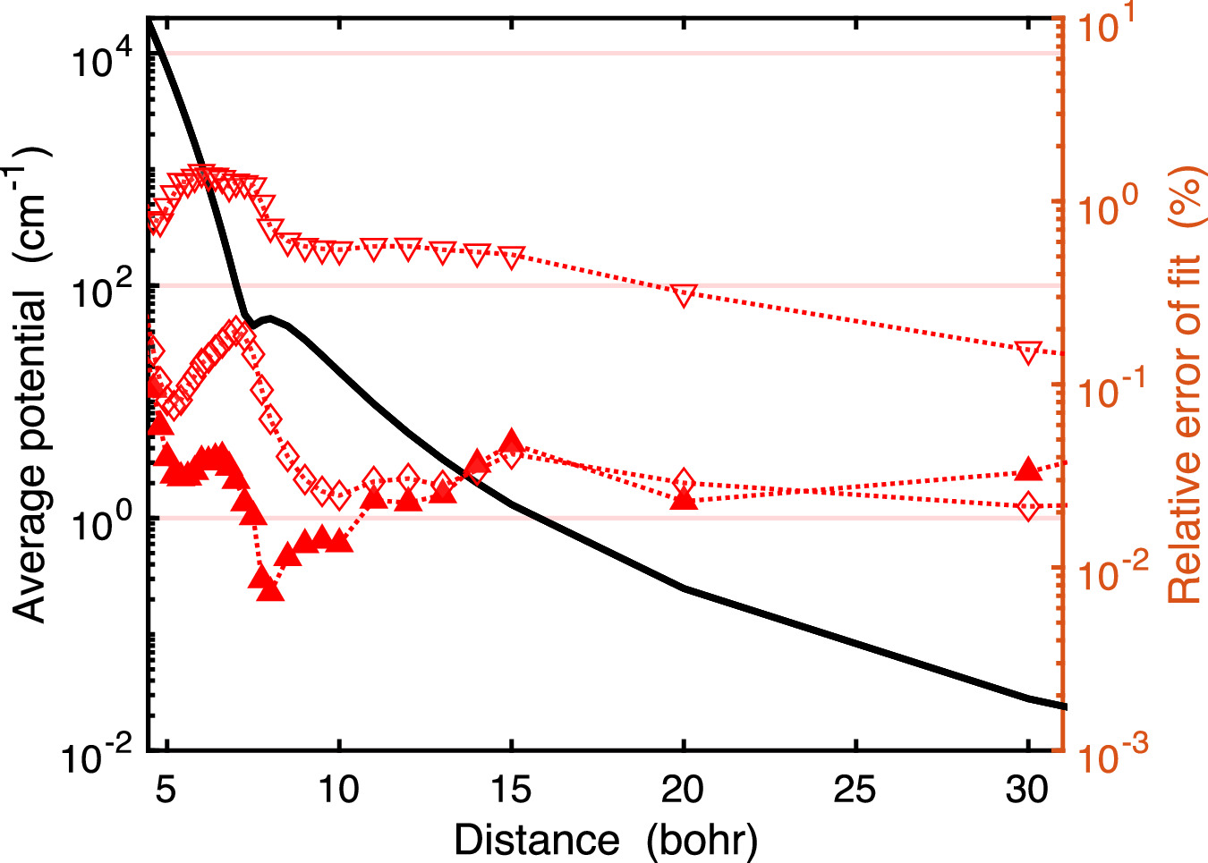
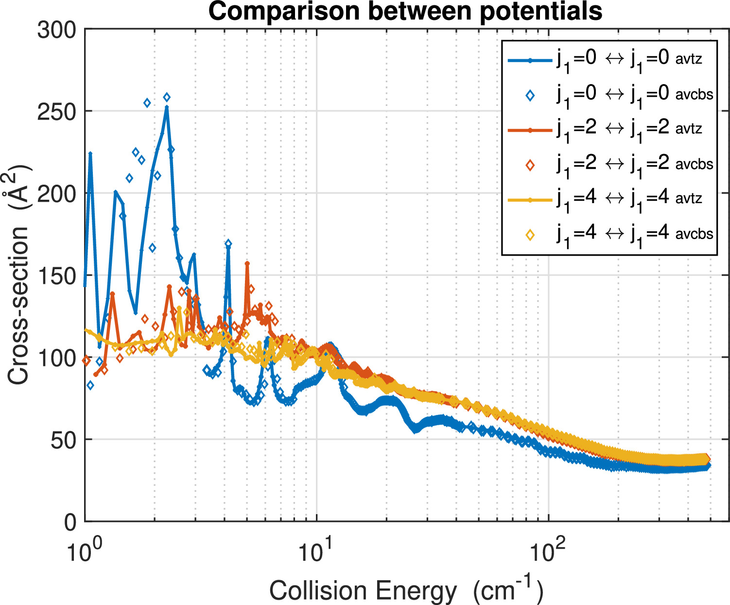
Figure B4. Pressure-broadening cross sections for the collision CO2–H2, σPB(Ecoll). Ortho- and para-H2 yield very similar results, except at very low energies (see inset).
Download figure:
Standard image High-resolution image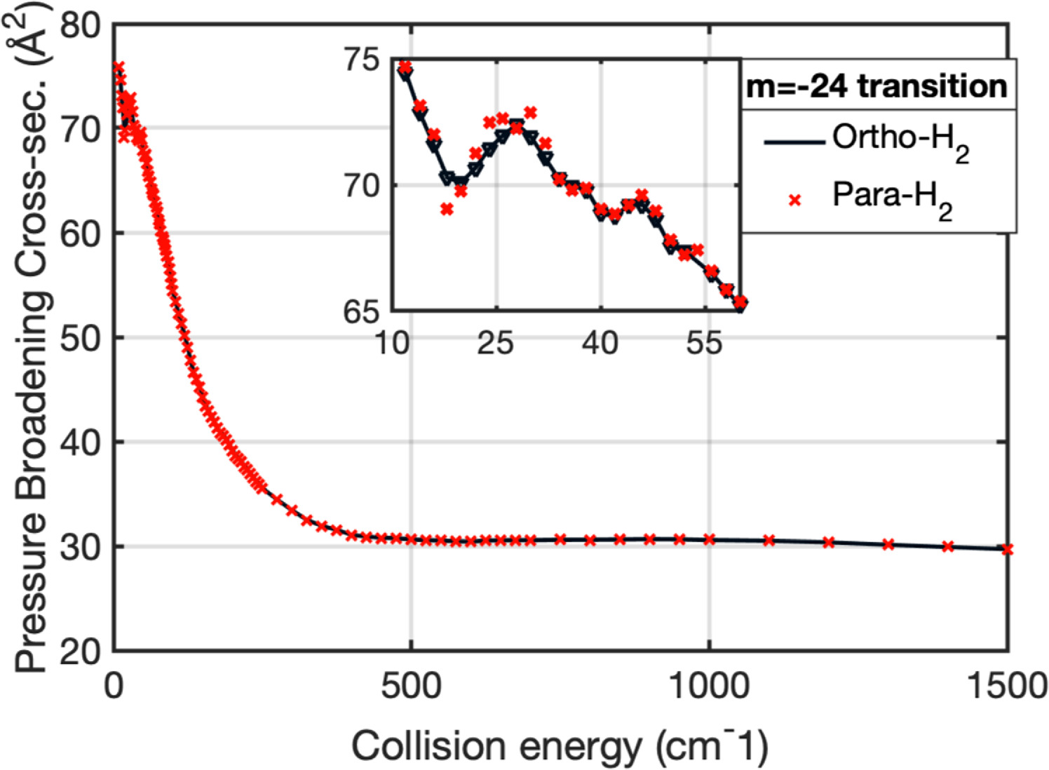
It must be underlined, though, that neither the smoothness of results nor the similarity of ortho- and para-H2 pressure-broadening cross sections need to remain true for all regimes. Because of the presence of high angular momentum for CO2, the collision studied here has a marked semiclassical character, witnessed by the behavior of the 3 − j and 6 − j symbols. The behavior at low j1 is expected to be much more quantum-like, as was observed repeatedly, for quadrupole-dominated collisions, e.g., F. Thibault et al. (2011), and even more so, for dipole-dominated collisions (M. Mengel et al. 2000; B. Drouin & L. Wiesenfeld 2012a). From knowledge of the σPB(Ecoll), sections, we define the Maxwell-averaged cross section and pressure-broadening coefficient in the usual manner:


where the kinetic average relative speed is  , with M being the reduced mass of the collisional system.
B.4.1. Precision Analysis
Given the acceptable error for retrievals (of the order of ±10%), we found it useful to compare the results shown in Figures B4 and 5 with alternative methods, more economical in computer time.
The first test we made was to apply the random-phase approximation to the σPB(Ecoll) computations, neglecting all interferences terms between the different channels (M. Baranger 1958; B. Drouin & L. Wiesenfeld 2012a; A. Faure et al. 2013). It is known that this approximation (see, e.g., the H2O–H2 case; A. Faure et al. 2013) is valid only for collision energies  , the minimum value of the potential. For the deep potential we have here (
 −220 cm−1, see Table B1), this approximation should not be not valid, and was indeed tested as being way too imprecise.
A second series of tests tried to disentangle the necessity of precise quantum mechanical methods for determining the potentials and precise fits of the potential points. In order to shorten computation, we only computed σPB(Ecoll), for Ecoll = 200 cm−1 (about 300 K). Precision study is not expected to change significantly the form of a full-fledged γ(T) computation, except for low-temperature results, which are much more potentially dependent, because of the occurrence of scattering resonances (B. Drouin & L. Wiesenfeld 2012a; A. Bergeat et al. 2020; see Figure B3). Remarkably, the σPB(Ecoll) value does not change at the 0.1% level of precision for the different methods of computing the PES (avtz up to avcbs).
Changes in the fitting procedure precision do have a limited influence on the results, of at most 2%. Fits with very few coefficients may sometimes make the dynamics diverge, and lead to nonphysical results; a compromise is necessary. However, it must be underlined that pressure shifts, as well as inelastic and elastic cross sections are much more sensitive to the details of the PES and fit. Also, there is now no indication if smaller values of ∣m∣ behave the same way (F. Thibault et al. 2011). Consequently, all data aside from pressure broadening should be carefully analyzed for convergence, as well as the influence of vibrational motion. Recall also that the inelastic cross sections averaged over the Maxwellian distribution of collision energies yield the population transfer rate coefficients (A. M. Arthurs & A. Dalgarno 1960; E. Roueff & F. Lique 2013), useful for population-level determination.
The relative insensitivity of σPB(Ecoll) (and hence of σPB(T)) to the details of the quantum computation conforms to the idea of scalability of this computational scheme, thanks to the possibility of using properly tailored computations. It may even be envisioned, for lower-quality results, that one resorts to approximate quantum scattering dynamical methods, based on Born first- or higher-order methods, and resorting to specific tests to validate approaches. For high enough ∣m∣ values, the insensitivity to the rotational state of H2 halves the computing time. The question of classical simulation (J.-M. Hartmann et al. 2018) of the dynamics should also be carefully examined, from the point of view of precision and scalability. It must be recalled, though, that for lower values of  and
 , some of the present conclusions do not hold as we remain in the quantum-dominated regime, where the whole quantum machinery must be performed.