


Abstract
We study quasi-normal f-mode oscillations in neutron star (NS) interiors within a linearized general relativistic formalism. We utilize approximately 9000 nuclear equations of state (EOSs) using spectral representation techniques, incorporating constraints on nuclear saturation properties, chiral effective field theory for pure neutron matter, and perturbative quantum chromodynamics for densities pertinent to NS cores. The median values of the f-mode frequency, νf (damping time, τf) for NSs with masses ranging from 1.4 to 2.0 M⊙ lie between 1.80 and 2.20 kHz (0.13–0.22 s) for our entire EOS set. Our study reveals a weak correlation between f-mode frequencies and individual nuclear saturation properties, prompting the necessity for more intricate methodologies to unveil multiparameter relationships. We observe a robust linear relationship between the radii and f-mode frequencies for different NS masses. Leveraging this correlation alongside NICER observations of PSR J0740+6620 and PSR J0030+0451, we establish constraints that exhibit partial and minimal overlap for observational data from Riley et al. and Miller et al., respectively, with our nucleonic EOS data set. Moreover, NICER data align closely with the radius and frequency values for a few hadron–quark hybrid EOS models. This indicates the need to consider additional exotic particles such as deconfined quarks at suprasaturation densities. We conclude that future observations of the radius or f-mode frequency for more than one NS mass, particularly at the extremes of the viable NS mass scale, would either rule out nucleon-only EOSs or provide definitive evidence in its favor.

Original content from this work may be used under the terms of the Creative Commons Attribution 4.0 licence. Any further distribution of this work must maintain attribution to the author(s) and the title of the work, journal citation and DOI.
1. Introduction
Neutron stars (NS) are among the densest objects existing in the present Universe with a measured and estimated mass in the range of 1–2 M⊙, confined in a sphere of radius ∼ 10 km. These tiny but massive stars harbor matter under extreme physical conditions that remain inaccessible to direct observation. Hence, our knowledge of an NS's interior, including the behavior of matter at such extreme densities, remains theoretical and is the subject of ongoing research and modeling. However, the new generations of telescopes have provided valuable observation data in the recent past and helped refine the theoretical description—called the equation of state (EOS). The EOS of matter inside an NS plays a critical role in determining various properties of the NS, such as its mass, radius, moment of inertia, tidal deformability, oscillation frequencies, and the structure of the internal layers. These are essential for understanding the observational characteristics of NSs, including their gravitational wave (GW) signals, electromagnetic radiation, and thermal emissions. The maximum observed mass of an NS, ∼2 M⊙, ruled out the softer EOS (Demorest et al. 2010; Antoniadis et al. 2013; Cromartie et al. 2019; Fonseca et al. 2021). The International Space Station–based X-ray telescope and instrument package, the Neutron Star Interior Composition Explorer (NICER; Gendreau & Arzoumanian 2017) measures the mass and radius of a pulsar simultaneously for the first time. Electromagnetic radiation from the hot spots at the magnetic poles of a rotating NS provide us with a direct route of observation when the radiation crosses our line of sight (Miller et al. 2021; Riley et al. 2021). The detection of GWs from NS mergers events have provided stringent limits on tidal deformability for an NS with a canonical mass of 1.4 M⊙, adding valuable insights into the EOS (Abbott et al. 2018). The nuclear physics data at the moderate densities combined with recent NICER observations can further improve existing constraints. Additionally, new X-ray observatories like the European Space Agency's Athena mission (Nandra et al. 2013) and NASA's Lynx mission (Kouveliotou et al. 2014) are expected to offer even higher-resolution X-ray observations of NSs. The third generation Einstein Telescope (Branchesi et al. 2023) will have a sensitivity 10 times better compared to second-generation detectors. Advanced LIGO and Virgo could be optimized for the detection of gravitational signals at low frequency. Ongoing and future surveys, such as the Square Kilometre Array (Kramer & Stappers 2015; Watts et al. 2015), are poised to discover more pulsars and provide a better understanding of the population of NSs and their properties. The coordinated observations of NS mergers at multiple wavelengths, such as X-rays, gamma-rays, and radio waves will definitely help enhance our understanding of the EOS of dense matter.
The NS core is believed to be made up of neutrons, along with an admixture of protons and leptons. There are several EOS models, which can be broadly categorized into nonrelativistic and relativistic models. Among them, the relativistic mean-field (RMF) model varieties have been successfully applied to study NS properties as well as finite nuclei properties. Over the decades additional mesons and nonlinear self-interaction as well as cross-coupling terms for all the mesons have been added to the original RMF, i.e., the Walecka (1974) Model. Various sets of tabulated RMF EOSs, compatible with recent astrophysical observations (Nandi et al. 2019), are available, 3 depending upon the form of interactions in the Lagrangian density. The associated couplings for the interactions are fitted to various nuclear matter parameters such as binding energy per particle, incompressibility, the symmetry energy coefficients and their derivatives, which are determined from terrestrial experiments at nuclear saturation density. Nevertheless the EOS provides a reasonable description of nuclear matter at suprasaturation densities. The nuclear matter parameters define the NS EOS and are correlated to NS observables (Agrawal et al. 2021; Ghosh et al. 2022; Pradhan et al. 2023a; Malik et al. 2023). At these high densities and extreme pressures, different models consider the possibility of strange matter like hyperons, quarks, and Bose–Einstein condensates (Banik et al. 2014; Char et al. 2015; Malik et al. 2021). It is a challenge to unravel the NS core composition and precisely determine its EOS owing to our limited knowledge of matter under extreme physical conditions.
In the absence of any universally acceptable model EOS, subject to limited observational data, several recent works have used spectral representations of realistic EOS as an accurate and efficient way of parameterizing the high-density sections of the NS EOS. (Abbott et al. 2018; Miller et al. 2019; Raaijmakers et al. 2020). This is a powerful theoretical tool, used to describe the EOS in terms of spectral functions, incorporating our current knowledge of fundamental physics. The tabulated version of the realistic EOS often infuses numerical errors in the calculation of the relevant thermodynamic quantities (Servignat et al. 2023). A robust analytic representation of the EOS like spectral representation (Lindblom 2010, 2018, 2022), generalized piecewise polytropic representation (O'Boyle et al. 2020), or speed of sound parameterization (Tews et al. 2018; Greif et al. 2019) becomes quite useful in scenarios where we need numerical determination of thermodynamic quantities associated with a cold β-equilibrated EOS at any arbitrary energy density inside the NS.
The structure parameters like mass, radius, and tidal deformability have taken crucial roles to address the uncertainties in NS EOS. Quasiperiodic oscillations are also valuable tools for studying compact objects and the processes occurring in their binary systems. NSs can exhibit a variety of oscillation modes mainly observed in the X-ray light curves of NSs in various types of binary systems, including low-mass X-ray binaries and NS X-ray binaries. A general relativistic description of oscillations due to nonradial perturbations involves what are called the quasi-normal modes (QNMs). Einstein equations govern the dynamics both inside and outside the star. QNMs are different than the normal modes describing Newtonian oscillations of matter inside the star. These modes are damped due to the emission of GWs from the star. The emitted GWs, given by the perturbations of the spacetime metric tensor, carry information about the internal structure and composition of the NS. The real part of the complex-valued QNM frequency represents the actual frequency of the oscillations, and the imaginary part corresponds to an exponential damping of the wave. Outside the star, determination of the frequency and damping time of the QNMs becomes an eigenfrequency problem subject to appropriate boundary conditions both at the surface of the NS and at spatial infinity. The internal structure and dynamics of the matter inside it influence the frequencies and damping times of the QNMs via the boundary condition at the surface of the NS. Inside the star, the oscillations of the matter and the GWs are coupled to each other via the Einstein equations.
The study of QNMs of oscillating astrophysical objects started with spherically symmetric black hole spacetimes (see Regge & Wheeler 1957; Vishveshwara 1970; Zerilli 1970) and was later extended to compact astrophysical stars (Thorne & Campolattaro 1967) including NSs (see the review by Kokkotas & Schmidt 1999 for references). The modes of oscillation inside the NS are characterized based on the physics behind the restoring force. For example, the pressure of the fluid (which is generally considered incompressible) in the NS interior acts as a restoring force for p-modes. Buoyancy restores the so-called gravity g-modes, which originate from internal temperature or composition gradients. The most fundamental mode of oscillation is the f-modes, which arise out of density perturbations. They typically have a frequency of around 2.4 kHz (Kokkotas et al. 2001; Rezzolla 2003) and have the strongest coupling with the emission of GWs. Determination of the eigenfrequencies while ignoring the metric perturbations during fluid oscillations (relativistic Cowling approximation) to simplify the calculations overestimates the frequency of certain fundamental modes (see the discussion on the accuracy of this approximation in Sotani & Takiwaki 2020). We can improve the accuracy by introducing the emission of GWs and using a post-Newtonian approximation to estimate the damping rate of the f-modes as a result. This way, one can obtain scaling relations between the bulk properties of the star, e.g., compactness, mass, moment of inertia, and mode frequency, and the damping time (Detweiler 1975; Andersson & Kokkotas 1996, 1998; Kokkotas et al. 2001; Benhar et al. 2004; Andersson 2019). When the problem is treated general relativistically, we get f-modes for the QNM.
Now, several works in the literature have demonstrated that for f-modes, the relativistic analysis also leads to very similar scaling relations. Such scaling relations can thus be taken as universal (see, for example, Andersson & Kokkotas 1996, 1998; Lattimer & Prakash 2001; Tsui & Leung 2005; Lau et al. 2010; Yagi & Yunes 2013). This feature of universality can be used as a landmark. One can check how well the calculated frequencies and damping times of the QNMs for a given EOS fit the scaling relations as a sort of consistency requirement (for details, see Andersson 2021). This is a strategy we consistently follow throughout this paper. Another feature of the NS, tidal deformability, also encodes important information about the shape of the star. An external tidal gravitational field acting on the NS contributes to the quadrupole and higher moments of the matter distribution inside (for more details, see Chan et al. 2014; Poisson & Will 2014; Andersson & Pnigouras 2020, 2021; Pratten et al. 2020).
Apart from the f-modes, there are also other modes that typically correspond to one or more additional physical processes. These modes mostly have frequencies higher than those of f-modes. For example, the frequency of the g-modes, which appear when the temperature and/or the pressure of the NS vary from one point inside the star to another, can lie in a range starting from the order of 100 kHz (Reisenegger & Goldreich 1992). For this reason, one expects g-modes to appear when a phase transition occurs inside the NS (Andersson 2019). Apart from these, p-modes and r-modes can also occur due to pressure and spin-related instabilities in the NS, respectively (for details, see the review by Andersson 2019 and the references therein). However, in this work, we focus only on f-modes for the NS, determining their frequencies and damping times from fully general relativistic calculations.
Recent publications (Sotani 2021; Kunjipurayil et al. 2022; Pradhan et al. 2022, 2023b) show efforts to estimate nuclear matter parameters using stellar oscillation modes. Pradhan et al. (2022) reported how the effective nucleon mass (m⋆) at saturation is correlated with the f-mode frequencies for a set of EOSs generated within the RMF formalism. A strong correlation of the stellar oscillation frequencies with symmetry energy parameters like Jsym,0, Ksym,0, Lsym,0, and so on would allow us to infer the composition of matter at very high densities in the NS interior (Patra et al. 2023).
In this work we have prepared a set of ∼9000 nucleonic EOSs though a Bayesian analysis of RMF model parameters. Constraints of recent interest like the chiral effective field theory (χEFT) and perturbative quantum chromodynamics (pQCD) at relevant energy densities are imposed to infer the parameter set. Then we determine a highly accurate spectral representation of the generated set and numerically solve the fully general relativistic perturbation equations for a set of equilibrium configuration NSs with varying mass for each EOS. We report the corresponding f-mode frequencies and the GW damping times over the EOS set and finally explore correlations of the frequencies and damping times with nuclear matter parameters and stellar observables.
The paper is organized in the following manner. Section 2 provides a brief overview of the RMF formalism for the nuclear EOS at zero temperature followed by a brief description framework for spectral fitting of the EOS, and the formalism for nonradial quadrupolar oscillations of a nonrotating NS. Section 3 contains the results for a set of parameterized spectral versions of the entire EOS set. We discuss the results and conclude our work in Section 4.
2. Formalism
2.1. Relativistic Mean-field Equation of State
We generate a set of EOSs within a description of nuclear matter based on a relativistic field theoretical approach where the nuclear interaction between nucleons is introduced through the exchange of the scalar–isoscalar meson σ, the vector–isoscalar meson ω, and the vector–isovector meson ϱ.
The Lagrangian density is given by (Dutra et al. 2014; Malik et al. 2023)

where

denotes the Dirac equation for the nucleon doublet (neutron and proton) with bare mass mN , Ψ is a Dirac spinor, γμ are the Dirac matrices, and t is the isospin operator. represents the mesons, which is given by


where F(ω,ϱ)μ ν = ∂μ A(ω,ϱ)ν − ∂ν A(ω,ϱ)μ are the vector meson tensors.

contains nonlinear terms with parameters b, c, ξ, and Λω to take care of the high-density behavior of the matter. The gi values are the couplings of the nucleons to the meson fields i = σ, ω, and ϱ, with masses mi . Finally, the Lagrangian density for the leptons is given as , where Ψl (l = e−, μ−) denotes the lepton spinor; leptons are considered noninteracting. The equations of motion for the mesons fields are obtained from Euler–Lagrange equations
![${{ \mathcal L }}_{\mathrm{leptons}}=\bar{{{\rm{\Psi }}}_{l}}\left[{\gamma }^{\mu }\left(i{\partial }_{\mu }-{m}_{l}\right){{\rm{\Psi }}}_{l}\right]$](https://content.cld.iop.org/journals/0004-637X/968/2/124/revision1/apjad43e6ieqn2.gif)


where and ρi are, respectively, the scalar density and the number density of nucleon i. The effect of the nonlinear terms on the magnitude of the meson fields is clearly shown through the following terms


and are solved using the RMF approximation with the constraint of β equilibrium, i.e., μn − μp = μe , where the μ values are the chemical potential of the respective particles. Also, total baryon number (np + nn ) conservation and the charge neutrality condition np = ne are enforced.
The pressure and energy density of the baryons and leptons are given by the following expressions

where for protons and neutrons and for electrons and muons, and kFi is the Fermi moment of particle i. The pressure is determined from the thermodynamic relation for every component


We generate our EOS set using a Bayesian setup with minimal constraints as done in Malik et al. (2023). These constraints include nuclear saturation properties such as a saturation density of ρ0 = 0.153 ± 0.005 fm−3, a binding energy per nucleon of e0 = −16.1 ± 0.2 MeV, a nuclear incompressibility of K0 = 230 ± 40 MeV, and a symmetry energy of Jsym,0 = 32.5 ± 1.8 MeV at the saturation density. Furthermore, we impose a low-density constraint for the pure neutron matter pressure from EFT (Hebeler et al. 2010) with twice the uncertainty and demand that the maximum NS mass corresponding to the EOS is above the observed 2 M⊙. Additionally, we employ a pQCD-derived constraint on the pressure at 8 times the baryon density (ns = 0.16 fm−3) for a pQCD scale X = 4 (Komoltsev & Kurkela 2022). Finally, we choose ∼9000 nucleonic EOSs for the present calculation from the posterior.
2.2. Spectral Representation of the Equation of State
We find the spectral parameters for our set of EOSs by fitting the tabular RMF EOSs with a spectral version. The methodology in Lindblom (2010) leads us to faithful representations of realistic EOSs for nuclear matter inside the NS by constructing spectral expansions of key thermodynamic quantities. Linear combinations of a complete set of functions like the Fourier basis functions allow us to expand a thermodynamic quantity like the adiabatic index, defined as

The coefficients of such basis functions in the expansion uniquely determine any given physically valid EOS. One can find that such a representation satisfies the basic necessary thermodynamic conditions. To obtain a pressure-based form, we expand the adiabatic index Γ(p) in terms of the basis functions Φk (p) as

We choose Φk (p) = Φk (x), where x is a dimensionless logarithmic pressure variable as in Lindblom (2010), and p0 is the minimum pressure where the high-density part of the EOS is joined to the low-density part of the Baym–Pethick–Sutherland (Baym et al. 1971) EOS. The γk values are the spectral coefficients.

Numerical integration of the following gives us  (p) for the obtained expansion of Γ(p)

where μ(p) is the chemical potential defined as

The energy density 0 at the minimum pressure p0 is the constant of integration. We match the low-density EOS at this pressure generally occurring at a number density slightly below the nuclear saturation density such that there is no unexpected phase transition at the junction. One can determine an empirical fit to any given EOS with arbitrary accuracy by increasing the number of basis functions used. There are four spectral coefficients corresponding to four basis functions as in Lindblom (2010) for fitting the set of RMF EOSs we are using. We plot the distribution of the spectral parameters γ0, γ1, γ2, γ3, and p0 in Figure 2. Apart from the coefficients, the parameters 0 and xmax have fixed values. We optimize the choice of spectral coefficients, γk
, by minimizing the differences between fit(xi
, γk
) and the energy density i
= (xi
) values from the tabular version of the EOSs for a specific set of x values (or p values). The following residual quantifies the faithfulness of the fitting

where we sum over the chosen pressure values between pmax is the pressure at the center of the nonrotating maximum-mass NS for the given EOS. The spectral version of the EOS serves as input for the Tolman–Oppenheimer–Volkoff equations, which give us the equilibrium configuration of the star.

2.3. Metric with Perturbations
To determine the frequencies of the f-modes, we solve the Einstein equations Gμ ν = 8π GTμ ν . We assume here that the GWs are perturbations of the static background spacetime metric for the nonrotating NS. The perturbed metric has the form

The time dependence of the perturbed metric components can be expressed by the factor ei ω t for a wave mode. Here ω is complex as the waves will decay due to the imposed open boundary conditions, which will be discussed shortly. The real part of ω is the oscillation frequency, while the imaginary part gives the inverse of the GW damping time (if it is positive) of the wave mode. These oscillations are studied considering the linearized Einstein equations, coupled with the equations of hydrodynamics, for our set of EOS, with suitably posed boundary conditions. A small perturbation hμ ν is assumed on a static spherically symmetric background metric given by

Here and with being the enclosed mass and pressure of the star at . Here H0, H1, and K are radial perturbations of the metric and the angular part is contained in the spherical harmonics with l denoting the orbital angular momentum number and m is the azimuthal number.

![${e}^{\nu (r)}\,=\exp \left(\displaystyle \frac{2G}{{c}^{2}}{\int }_{0}^{r}\left\{\displaystyle \frac{m(r^{\prime} )+\tfrac{4\pi p(r^{\prime} )r{{\prime} }^{3}}{{c}^{2}}}{r^{\prime} \left[r^{\prime} -\tfrac{2m(r^{\prime} )G}{{c}^{2}}\right]}\right\}{dr}^{\prime} \right){e}^{{\nu }_{0}};$](https://content.cld.iop.org/journals/0004-637X/968/2/124/revision1/apjad43e6ieqn9.gif)


2.4. Lindblom–Detweiler Equations
The perturbations of the energy–momentum tensor of the fluid also need to be taken into account in the Einstein equation. The components of the Lagrangian displacement vector ξa (r, θ, ϕ) describe the perturbations of the fluid inside the star


where W and V are functions with respect to r that describe fluid perturbations. Fluid perturbations exist only inside the star. The introduction of a new variable X leads to simplification of the perturbation equations for the NS interior. X is related to the rest of the perturbation functions through the following equations


where n = (l − 1)(l + 2)/2, b = Gm/rc2, Q = b + 4π
Gr2
p/c4, and is the local energy density. The GW equations can be written as a set of four coupled linear differential equations for the four perturbation functions H1, K, W, and X, which do not diverge inside the star for any given value of ω (Lindblom & Detweiler 1983)


where is the equilibrium speed of sound of NS matter undergoing oscillations.

2.5. Boundary Conditions for the Perturbation Equations
We discuss the boundary conditions imposed here to solve the Einstein equations inside the star. For that, one needs to integrate the perturbation equations from the center of the star to a certain radius inside the star. The boundary condition for the perturbation functions at the center of the star r = 0 are

The condition Δp = 0 at r = R, the star's surface, requires the perturbation function X to be equal to 0 at the surface of the star. We assign some small arbitrary values to the functions H1, K, and W at the star's surface and integrate backward to reach the point at which the integration from the center of the star ends and join the two forward and backward solutions. To find the QNM frequency for a given star, we solve the Zerilli equation given as (Fackerell 1971; Lindblom & Detweiler 1983)

where and VZ (r) is the effective potential outside the star(r ≥ R). The value of the Zerilli function Z(r⋆), as given in Equation (20) of Kunjipurayil et al. (2022), depends only on H1 and K as the fluid perturbations W, V, and X become nonexistent outside the star. We calculate the value of Z(r*) at the surface of the star from the values of H1 and K at the surface. Outside the star Equation (26) is numerically integrated starting from the surface as done in Kunjipurayil et al. (2022) and Zhao & Lattimer (2022) until a distance equivalent to r = 25ω−1. We match this value of Z at r = 25ω−1 with that obtained from an asymptotic expansion of Z valid far away from the surface of the NS. We impose the outgoing boundary condition, which requires the amplitude of incoming GWs far away from the surface of the star to be zero (Lindblom & Detweiler 1983) and solve for ω as done in Kunjipurayil et al. (2022) and Zhao & Lattimer (2022).

3. Results
Our primary aim is to comprehensively examine the f-mode oscillations, one of the nonradial oscillatory modes of NSs over a broad range of realistic EOSs. To achieve this, we employ a linearized and fully general relativistic approach. For this work, we prepare a set of realistic nuclear EOSs that only have nucleonic composition, obtained with the RMF approach. We utilize around 9000 nucleonic EOSs that were acquired through Bayesian inference with minimal restrictions imposed on them, as previously mentioned in Section 2.1. The ranges of nuclear saturation properties, including the binding energy e0, nuclear incompressibility K0, skewness parameter Q0, symmetry energy Jsym,0, its slope Lsym,0, and its curvature Ksym,0 at the saturation number density n0, are presented in Table 1.
Table 1. Nuclear Matter Parameters Calculated at Saturation Density for the 9000 Equations of State Used in This Work, along with the Median and 90% Confidence Interval
| Model | e0 | n0 | K0 | Q0 | Jsym,0 | Lsym,0 | Ksym,0 | m⋆ |
|---|---|---|---|---|---|---|---|---|
| (MeV) | (fm−3) | (MeV) | (MeV) | (MeV) | (MeV) | (MeV) | ||
| NL |


Download table as: ASCIITypeset image
Our tabulated set of EOSs is given a functional representation by the spectral decomposition method (see Section 2.2). This is a reliable approach which is often used in the context of NS interior structure calculations. Using a minimal number of spectral coefficients, we achieved a fit of all our ∼9000 EOS with a precision of less than 0.5% using the Levenberg–Marquardt method for optimization of the residual errors in Equation (14) as done in Lindblom (2010, 2018).
In Figure 1, we plot the entire EOS set employed in this work and compare with constraints derived from pQCD at baryon densities of 5ns and 8ns , with ns = 0.16 fm−3. The plot is divided into two panels, representing two different renormalization scales, (X = 1) and (X = 4), for the pQCD constraints. The left panel focuses on the renormalization scale (X = 1) of the pQCD constraints, with the green patch indicating the energy densities and pressure points for each EOS at the respective baryon densities that are in agreement with the pQCD constraints. All the EOSs in our set meet the requirements set by the pQCD results up to 8ns and a renormalization scale of four. However, the central density for maximum-mass NS for all the EOS in our set is below 7ns .

Figure 1. We display the pressure and energy density for the employed EOS set, enclosing areas compliant with pQCD-derived restrictions for baryon number densities equal to 5ns and 8ns (where ns = 0.16 fm−3; Komoltsev & Kurkela 2022) by red dashed lines, informed by the stringent renormalization scale parameter, X = 1 (X = 4), according to Kurkela et al. (2010) in the left panel (right panel). We indicate the energy densities and pressures that satisfy the pQCD constraints by green patches for the corresponding number densities. It will be significant to note the central density for the maximum-mass NS within 7ns across our entire EOS set.
Download figure:
Standard image High-resolution imageIn Figure 2, we present a corner plot showing the distributions of the spectral parameters for our set of EOSs. This visual representation is essential to understand the statistical properties and correlations among the parameters. The diagonal plots contain representations of the marginalized 1D distributions of the individual parameters, while the off-diagonal plots illustrate the 2D distributions for pairs of parameters, giving insight into their mutual relationships. The median value of each spectral parameter along with error are shown as a label on the corresponding diagonal plot and the dashed vertical lines mark the limits of the 68% confidence interval (CI) of the parameter. The color gradient, which changes from dark to light blue in the 2D graphs, symbolizes the CIs 1σ, 2σ, and 3σ. The elliptical shapes observed in the 2D plots indicate strong correlations among the parameters. If the shape approaches a circle, it signifies a weak correlation between the given parameter pair.

Figure 2. The corner plot shows the distributions of parameters γ0, γ1, γ2, γ3, and p0 for the spectral representation of the EOSs within the acquired set of RMF EOSs used for this study. Vertical lines indicate the 68% CIs, while varying shades in the 2D distribution denote the 1σ, 2σ, and 3σ CIs.
Download figure:
Standard image High-resolution imageAn interesting observation from the figure is that most of the γi parameters show strong correlations with their subsequent γi+1 parameters. This trend is expected; to ensure a smooth EOS, an increase in a particular γ must be related to the previous one. This aspect of parameter correlation is essential for maintaining a coherent and smooth representation of the EOS, thus confirming the effectiveness of the spectral decomposition format in capturing the essential characteristics of the dense matter EOS.
In Figure 3, we plot the mass–radius (MR) relation of the NS (left) and the mass–tidal deformability (right) of all EOSs considered using the spectral representation of the EOSs (see Section 2.1). The gray zones in the left panel represent the 90% (dark) and 50% (light) CIs for the binary components of the GW170817 event (Abbott et al. 2019). The predictions of NS radius measurements from NICER X-ray data for the PSR J0030+0451 and PSR J0740+6620 pulsars are also included, with the 1σ (68%) confidence zone of the 2D posterior distribution in the MR domain of the millisecond pulsar PSR J0030+0451 shown in brown and yellow from Riley et al. (2019) and Miller et al. (2019), respectively, and PSR J0740+6620 is shown in magenta (Miller et al. 2021; Riley et al. 2021). Finally, the blue bar in the left panel represent the 90% CI radius of a 2.08 M⊙ NS as reported in Miller et al. (2021), who combined NICER data and X-ray observations. The blue bar in the right panel shows the bounds on the tidal deformability of a 1.36 M⊙ NS as given in Abbott et al. (2018). All MR curves have a maximum mass greater than 2 M⊙, since this was imposed as a constraint during Bayesian sampling. Despite the dearth of constraints on radius and tidal deformability during sampling, the predictions of NS mass and radius are well within the observational bounds over the entire EOS set with the minimal requirements that were set. The obtained radius of a 1.4 M⊙ NS in our set is 12.03–13.20 km, and the deformability of the tidal channel for a 1.36 M⊙ star is 431–659 within the 90% CI. The maximum mass of the NS ranges from 2 to 2.25 M⊙, which is consistent with the results reported in Rezzolla et al. (2018). It is worth noting that we applied pQCD constraints to our EOS set, which limited the maximum mass of the NS to a certain range and eliminated some of the stiffer EOSs.

Figure 3. The NS MR and mass–tidal deformability curves are plotted for the entire set of EOSs used in this work. The gray zones in the left panel indicate 90% (dark) and 50% (light) CIs for the binary components of the GW170817 event (Abbott et al. 2018). The brown and yellow zones in the same panel represent the credible zone 1σ (68%) of the 2D posterior distribution in the MR domain of millisecond pulsar PSR J0030+0451 in Riley et al. (2019) and Miller et al. (2019), respectively, while the magenta zone is for PSR J0740+6620 (Miller et al. 2021; Riley et al. 2021) based on NICER X-ray data. The blue bars represent the 90% CI radius of PSR J0740+6620 at 2.08 M⊙ (left panel) from Miller et al. (2021) and the tidal deformability from the GW170817 event (Abbott et al. 2018) at 1.36 M⊙ (right panel).
Download figure:
Standard image High-resolution imageWe display the f-mode frequencies in Figure 4 (left) versus NS mass. They increase from 1.6 to 2.6 kHz for variations of the NS mass from 1.2 to 2.25 M⊙. It is worth noting that the f-mode frequency within the Cowling approximation for NSs with a mass greater than 2 M⊙ is in the range of 2.1–2.7 kHz and 2.3–2.65 kHz for the two types of EOSs used in Kumar et al. (2023), respectively. It is a widely known fact that the calculation of the f-mode frequencies using the Cowling approximation overestimates them by up to 10% to 30% for NSs with masses ranging from 1.0 to 2.5 M⊙, when compared to the frequency obtained from the linearized general relativistic formalism (Benhar et al. 2004; Doneva et al. 2013; Pradhan et al. 2022). In the right panel, we plot the distribution of f-mode frequencies for NS masses ranging from 1.4 to 2.0 M⊙. The distribution for a given mass is accompanied by its median value and the 90% CI bounds. This variation in the f-mode frequencies across various NS masses is indicative of the current understanding of the EOSs for NSs. The measurements of f-mode frequencies (with precision beyond the current uncertainty of approximately 0.2 kHz) by next-generation detectors could potentially lead to a more refined understanding of the EOS domain for NS interiors.
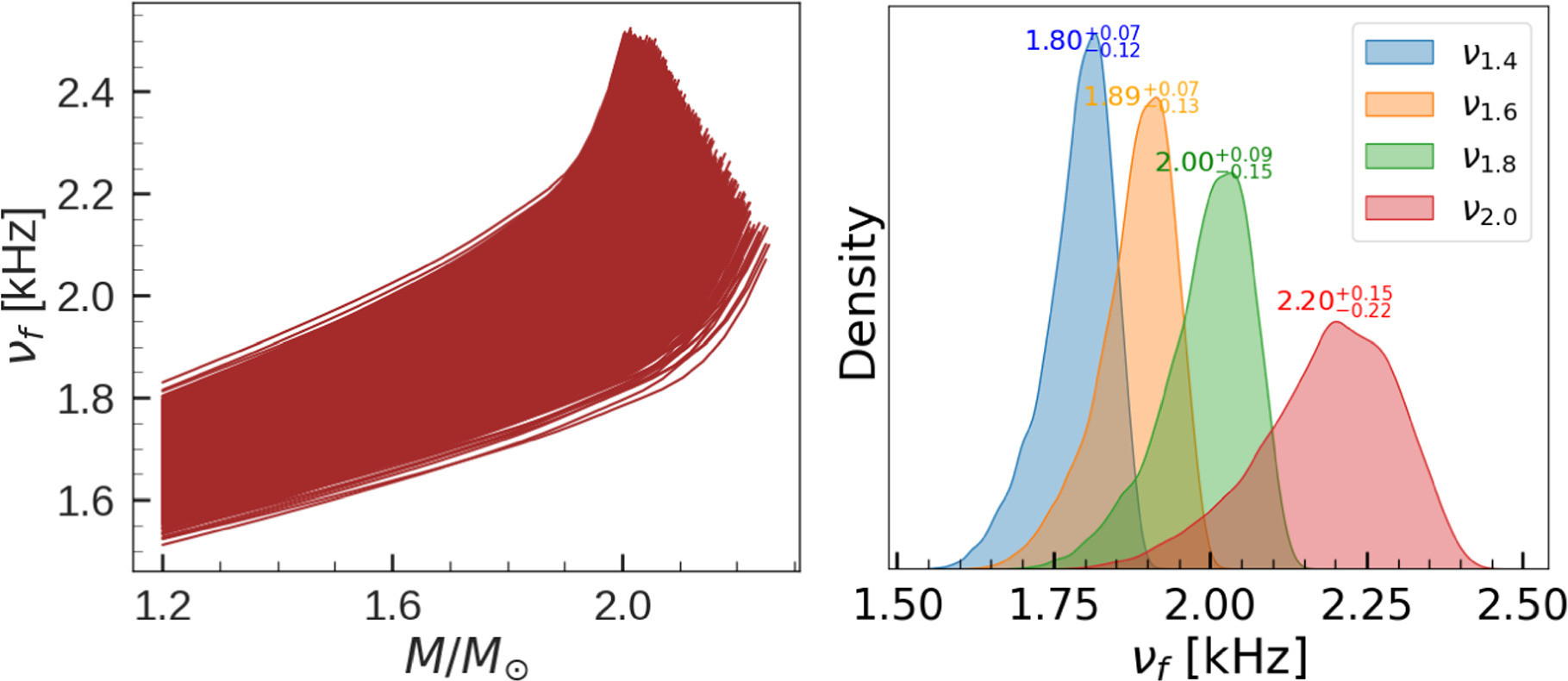
Figure 4. The frequency of the f-mode oscillations, calculated using linearized general relativity, is shown on the left for the EOS set utilized. On the right, the density distribution of the f-mode frequency for NS masses in the range of 1.4–2.0 M⊙ is plotted.
Download figure:
Standard image High-resolution imageNext we calculate the GW damping times corresponding to the f-mode frequencies for our EOS set. The inverse of the imaginary part of ω in the metric perturbations gives us the damping time as discussed in Section 3. In Figure 5 we plot the variation of damping times with stellar mass. We obtain a monotonically decreasing trend for the damping times with an increase in NS mass until the maximum mass for all EOSs. The damping time of a 1.4 M⊙(2.0 M⊙) NS lies between 0.20 and 0.25 s (0.13–0.15 s). The range of damping times in this work, for the two NS masses mentioned, is in good agreement with the range of damping times reported in Pradhan et al. (2022) for their set of RMF EOSs.

Figure 5. Plot of the GW damping time τf for the corresponding f-mode oscillation as a function of stellar mass for the 9000 RMF EOS set used in this work.
Download figure:
Standard image High-resolution imageIn Figure 6 we explore the linear dependence between various spectral parameters, nuclear saturation properties, the pressure of NS matter at 2 and 3 times the fixed baryon density ns , and other NS properties. We also examine how the frequency of the f-mode oscillation for different masses relates to the individual components of our nuclear EOS set. We calculate the Pearson correlation coefficients between these quantities using the entire ∼9000 EOS set. The heat map's color spectrum, ranging from green to red, indicates the strength of the correlation, from negative to positive, respectively. A deeper red (green) hue indicates a stronger positive (negative) correlation, with a magnitude of coefficients above 0.8 indicating a particularly strong linear relationship. The correlation between the spectral parameters γ1, γ2, and γ3 is exceptionally high, clearly indicating a linear relationship between them. This is also true for the pair m⋆ and the γi , suggesting that the effective mass of the nucleon has a strong influence on these spectral parameters. Another finding is the strong correlation, greater than 0.9, between P(2ns ) and P(3ns ), which is the pressure β at 2 and 3 times ns and various properties of the NS such as radius, deformability of the tidal, frequency of the f-mode, and damping time for NS masses of 1.4 M⊙ and 2.0 M⊙. This suggests a considerable degree of linear dependence between the properties of NSs of different masses and the overall EOS, rather than individual nuclear saturation properties. It is worth emphasizing the strong correlation previously reported in Pradhan et al. (2022) between the fundamental f-mode frequency of different NS masses and the effective nucleon mass at saturation m⋆ appears to be less pronounced in our study using the chosen set of EOSs. This difference can be mainly attributed to certain choices regarding the set of EOSs. The set employed in our research was generated through Bayesian inference subject to constraints. Specifically, constraints from χEFT for our low-density pure neutron matter and pQCD at 8 times ns were included. These constraints were not considered by the other authors. An additional notable distinction is the inclusion of an interaction ω4 in the Lagrangian that we studied. It is important to note that this ω4 term tends to soften the EOS, which is a characteristic favored by pQCD analysis (Malik et al. 2023). The heat map suggests that the maximum radius of the NS is closely related to its R1.4, R2.0, and f2.0 values. Furthermore, the f-mode frequencies of NSs with 1.4 M⊙ and 2.0 M⊙ are strongly correlated with their tidal deformabilities Λ1.4 and Λ2.0, respectively, providing insight into how the internal structure of the NS responds to tidal forces.
Asteroseismology, the study of stellar oscillations, allows us to infer global NS properties such as mass, radius, and average stellar density from f-mode frequencies and the GW damping time through certain empirical relations. We describe the results for some selected relations in the following paragraphs.

Figure 6. Heat map displaying the Pearson correlation coefficients among the spectral parameters (γ0, γ1, γ2, and γ3), nuclear matter parameters (m⋆, K0, Q0, etc.), pressure at multiples of the saturation number density ns = 0.16 fm−3, and stellar observables like mass, radius, f-mode frequency, etc. Subscripts with the corresponding NS property stand for the NS mass associated with that property.
Download figure:
Standard image High-resolution imageIn Figure 7 we plot the data with a straight line fit using

This empirical relation is well known since the publication of Andersson & Kokkotas (1998). We find the slope a to be 35.94 ± 0.0113 kHz km and the intercept b to be 0.6260 ± 0.0004 kHz. We can compare these values with the values reported in Pradhan et al. (2022; see Table 2). They calculated the f-mode frequencies with a different set of RMF EOSs and found the slope equal to 36.20 kHz km and the intercept equal to 0.535 kHz. Kumar et al. (2023) report the same coefficients with values a = 22.27 and 26.76 and b = 1.520 and 1.348 corresponding to determination of f-modes with the Cowling approximation for a set of hybrid and a set of purely nucleonic EOSs with density-dependent couplings. The values for a and b thus appears to be dependent on the set of EOSs considered, which makes the empirical Equation (27) somewhat EOS dependent. The relative percentage error for the aforementioned fit in this work is 2.84%.

Figure 7. Empirical relation between the f-mode frequency with the average stellar density (left panel) and that between the corresponding dimensionless GW damping time and the stellar compactness for the set of 9000 RMF EOSs used in this work. Stellar mass M, radius R, and damping time τf are in kilometers.
Download figure:
Standard image High-resolution imageTable 2. Coefficients of the Fitting Equation for the Empirical Relation in Equation (27)
| [Full General Relativity] | [Full General Relativity] | [Cowling] | |||
|---|---|---|---|---|---|
| Empirical Relation | Fitting Function | Coefficients of the Current Work | Relative Error | Coefficients of Pradhan et al. (2022) | Coefficients of Kumar et al. (2023) |
| ax + b | a = 35.94 ± 0.0113 | 2.84% | a = 36.20 | a = 22.27, 26.76 | |
| b = 0.6260 ± 0.0004 | b = 0.535 | b = 1.520, 1.348 |

Download table as: ASCIITypeset image
We display another empirical relation

in the right panel of Figure 7. τf is the GW damping time, equal to the inverse of the imaginary part of ω. Andersson & Kokkotas (1998) mentioned the existence of this scaling between a dimensionless damping time and compactness for the first time. Both the coefficients a and b are dimensionless and we find the following values (see Table 3) of a = −0.3051 ± 0.0001 and b = 0.0939 ± 3.0 × 10⁻⁵ with a relative error of 0.29%. Pradhan et al. (2022) reported the values of a = −0.245 and b = 0.080. These empirical relations have poor validity beyond M/R > 0.25 (Tsui & Leung 2005).
Table 3. Coefficients of the Fitting Equation for the Empirical Relation in Equation (28)
| [Full General Relativity] | [Full General Relativity] | |||
|---|---|---|---|---|
| Empirical Relation | Fitting Function | Coefficients of the Current Work | Relative Error | Coefficients of Pradhan et al. (2022) |
| ax + b | a = −0.3051 ± 0.0001 | 0.29% | a = −0.245 | |
| b = 0.0939 ± 3.0 × 10⁻⁵ | b = 0.080 |

Download table as: ASCIITypeset image
Kumar et al. (2023) have reported a new scaling between the f-mode frequency and the radius for an NS of given stellar mass

where x is the mass of the NS in M⊙ units. We plot the relation with our results of f-mode frequencies for 1.4 M⊙ and 2.0 M⊙ in Figure 8.
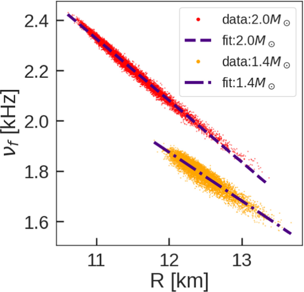
Figure 8. The empirical relation between the radii and the corresponding f-mode frequencies for the set of 9000 RMF EOSs used in this work. The orange (red) dots denote f-mode frequencies for an NS with 1.4 (2.0) M⊙. The dashed–dotted (dashed) line represents a linear fit based on Equation (29) for data for 1.4 (2.0) M⊙.
Download figure:
Standard image High-resolution imageWe find values (see Table 4) of a = −0.1933 ± 0.0008 kHz km−1 and b = 4.195 ± 0.010 kHz for 1.4 M⊙ and a =−0.2455 ± 0.0003 kHz km−1 and b = 5.027 ± 0.003 kHz for 2.0 M⊙. The maximum relative errors are 1.86% and 1.18%, respectively. The slope reported in Kumar et al. (2023) for masses over the range 1.6–2.4 M⊙ is around −0.22 kHz km−1 and the intercept is around 5.1 khz with a 1.5% relative error. A general relativistic treatment of the stellar oscillations in this work presents us with two different slopes for the two cases. This difference is due to the overestimation of f-mode frequencies that occurs when one employs Cowling approximation, as done in Kumar et al. (2023). From a specific observed value of the f-mode frequency for 1.4 M⊙, we can infer a smaller value of the radius from the fit in this work as compared to the fit in Kumar et al. (2023).
Table 4. Coefficients of the Fitting Equation for the Empirical Relation in Equation (29)
| [Full General Relativity] | [Cowling] | |||
|---|---|---|---|---|
| Empirical Relation | Fitting Function | Coefficients of the Current Work | Relative Error | Coefficients of Kumar et al. (2023) |
| f1.4–R1.4 | ax + b | a = −0.1933 ± 0.0008 | 1.86% | |
| b = 4.1949 ± 0.0095 | a = −0.22 | |||
| f2.0–R2.0 | ax + b | a = −0.2455 ± 0.0003 | 1.18% | b = 5.1 |
| b = 5.0268 ± 0.0034 |
Download table as: ASCIITypeset image
Motivated by the study in Lin & Steiner (2023), we also look into the correlation between the radii as well as f-mode frequencies of two extreme-mass NSs, utilizing our nucleonic EOS set. In Figure 9, we show a scatter plot of the radii (f-mode frequencies) of NSs with masses of 1.34 M⊙ and 2.07 M⊙ on the left (right). On both the panels, a strong correlation is noticed, with a Pearson's correlation coefficient of approximately 0.9 for our EOS set. In the left panel, the red dashed line indicates the most probable region of the joint posterior distribution of the NICER radii measurements of PSR J0740+6620 and PSR 0030+0451 calculated in Lin & Steiner (2023). The authors have claimed a 48% probability (with a 5% false alarm rate) of identifying a strong and sharp phase transition by applying their method to NICER observations. We note how our entire nucleonic set overlaps with the most probable region within the red dashed line. In the same panel, the area marked with the blue dashed line represents the constraints after we impose a strong correlation of 0.9 among the radius data in the NICER observations of the pulsars PSR J0740+6620 and PSR 0030+0451. NICER's 1σ posterior distributions are used to obtain this constraint. This method is based on data reported in Riley et al. (2019, 2021). To be more specific, we produce 2000 random samples of R1.34 and R2.07 within the 1σ range of the NICER observed values marginalized over NS masses and implemented a correlation of approximately 0.9 between the two radii. The plot shows a noticeable difference in the slope of the data points corresponding to a nucleonic EOS and those derived from NICER observations.

Figure 9. The relationship between the radii (left panel) and the f-mode frequencies (right panel) of NSs with masses of 1.34 M⊙ and 2.07 M⊙ for the EOS set used in this work. The dashed blue line on the left shows the NICER constraint, which was determined by taking the 1σ posteriors of the radius values from NICER measurements of PSR J0740+6620 and PSR 0030+0451 and marginalizing them over the NS masses while taking into account the correlation between them, based on the data in Riley et al. (2019, 2021). The area inside the red dashed boundary is the most probable region of the joint posterior distribution of the NICER radii measurements as in Lin & Steiner (2023). On the right, we inferred f-mode frequencies from the data in the radius domain using the universal relation in Equation (29) (see text for details). The red stars in the left panel (right panel) mark the calculated values corresponding to radii (f-mode frequencies) for a set of hybrid EOSs (Baym et al. 2018, 2019; Kojo et al. 2022), which support a hadron–quark phase transition.
Download figure:
Standard image High-resolution imageIn the right panel, we translate the NICER data from Riley et al. (2019, 2021) as well as those from Lin & Steiner (2023) in the radius domain using Equation (29) to obtain the corresponding constraints on the f-mode frequency domain. Note that the universal relation presented in Table 4 applies to NS masses of 1.4 M⊙ and 2.0 M⊙. For Figure 9 we calculate the relations for NS masses of 1.34 M⊙ and 2.07 M⊙. The slope and the intercept values are very close to those presented in Table 4: −0.1794 (−0.2360) kHz km−1 and 3.9891 (4.9283) kHz for an NS mass of 1.34 (2.07) M⊙. The nucleonic EOS set exhibits a similar overlap between the radius and frequency domains with the NICER-inferred constraint from the data in Riley et al. (2019, 2021). However, the partial overlap between the nucleonic EOS set and this NICER bound suggests that only nucleonic degrees of freedom for larger NS masses may not be sufficient enough to explain the observations.
In Figure 10, we present a similar analysis as in Figure 9 for NS masses 1.44 M⊙ and 2.07 M⊙ but determine the NICER constraints from the data published by Miller et al. (2019, 2021). The slope and the intercept values for a 1.44 M⊙ are −0.1869 kHz km−1 and 4.1215 kHz, respectively. We observe a clear distinction between the NICER bound and the nucleonic EOS set in both the radius and frequency domains. This finding further strengthens the conclusion drawn from the previous figure.

Figure 10. The relationship between the radii (left panel) and the f-mode frequencies (right panel) of NSs with masses of 1.44 M⊙ and 2.07 M⊙ for the EOS set used in this work. The dashed blue line on the left shows the NICER constraint, which was determined by taking the 1σ posteriors of the radius values from NICER measurements of PSR J0740+6620 and PSR 0030+0451 and marginalizing them over the NS masses while taking into account the correlation between them, based on the data in Miller et al. (2019, 2021). On the right, we inferred f-mode frequencies from the data in the radius domain using the universal relation in Equation (29) (see text for details). The red stars in the left panel (right panel) mark the calculated values corresponding to radii (f-mode frequencies) for a set of hybrid EOSs (Baym et al. 2018, 2019; Kojo et al. 2022), which support a hadron–quark phase transition.
Download figure:
Standard image High-resolution image
To investigate further, we utilize 12 EOS models with a maximum NS mass above 2.0 M⊙ by simulating a hadron–quark phase transition inside the NS core from the CompOSE database, such as VQCD (Jokela et al. 2021), QHC21-AT (Kojo et al. 2022), QHC19-C (Baym et al. 2019), QHC21-BT, QHC21-D, QHC19-D, QHC21-CT, QHC21-B, QHC21-C, QHC18 (Baym et al. 2018), QHC19-B, and QHC21-DT. The red stars in both Figures 9 and 10 with the label "Hyb-EOS" in both panels are the calculated values for these EOSs in the corresponding domains. It is clear that all the red stars fit comfortably within our NICER-derived constraints, as determined by both Riley et al. (2019, 2021) and Miller et al. (2019, 2021), over the radius and the f-mode frequency domains. The possibility of a hadron–quark phase transition or other exotic degrees of freedom in the NS EOS appears to be promising. Please be aware that the blue dashed contours derived from the NICER data for the pulsars PSR J0030+0451 and PSR J0740+6620, whether in the radius domain or in the f-mode frequency domain, are calculated using a correlation of 0.9 between the radii of NSs with these two masses, and are entirely dependent on the nucleonic degrees of freedom. Examining the differences in these correlations with other exotic degrees of freedom is a subject for future research and is not within the purview of this study.
The universal relation in Equation (29) acts as a tool to compare data from two different channels: X-ray channel and GW channel. Observations of thermal emission from hot spots on pulsars provide an effective way of measuring the NS radius. Parameter estimation of parameterized models of NS EOSs using such radius measurements (Raaijmakers et al. 2021) allows us to narrow down viable EOSs by putting constraints on the relevant parameters. Radius measurements from X-ray data are essentially based on X-ray pulse profile modeling (Bogdanov et al. 2021). This involves making assumptions about the stellar atmosphere and the EOS of matter inside the star itself. In short, such measurements are model dependent. f-mode observations offer a more direct path to probe the NS EOS by measuring the bulk properties of the star through its response to gravity. Thus, X-ray observations, while valuable, require additional assumptions about the star's surface and internal structure, making them less direct for studying the deep core where the EOS is truly uncertain as yet. These observations work best together (Yunes et al. 2022), with X-rays providing complementary data points like mass and radius to refine the interpretation of the NS EOS extracted from GWs (Psaltis et al. 2014).
4. Conclusion
We have carefully calculated the QNM frequency, specifically focusing on the f-mode oscillations of NSs. This analysis was conducted using a linearized approach to full general relativity, which allowed for a detailed examination of these oscillations. In our study, we utilized a wide range of nuclear EOSs (9000), derived through Bayesian inference. These EOSs were subjected to a few constraints. First, they conform to the minimal constraints on nuclear saturation properties. Second, they incorporate constraints from χEFT relevant to low-density pure neutron matter. Additionally, constraints derived from pQCD at densities pertinent to the cores of NSs were also applied. Finally, our selection of EOSs ensured that the NS maximum mass was above 2 M⊙, aligning with current astrophysical observations and theoretical predictions.
We then determine the spectral representation of our EOS set, which is one of the most widely accepted and optimal way to adapt any realistic EOS table into a functional form. This helps to reduce the computation time when calculating NS properties and is convenient for other astrophysical calculations. The MR and mass–tidal deformability relationships of NSs were calculated, and a detailed examination of the correlation among spectral parameters, various nuclear saturation properties, and NS properties was conducted. Empirical relations for f-mode frequencies and GW damping times were also explored, providing valuable insights into the composition of these compact objects.
One of the key findings is that the f-mode frequencies do not show a strong relationship with any single nuclear saturation property of the EOS when the 9000 EOSs are used. In fact, we find that some of the strong correlations reported in recent publications have become weak for our EOS set. This observation suggests that a more nuanced approach, possibly involving a multiparameter correlation analysis using machine learning techniques, might be necessary to unravel these complex relationships.
Interestingly, for NS with masses ∼ 1.4 M⊙ and ∼2.0 M⊙, we notice a strong correlation between their radii as well as f-mode frequencies. Using this correlation alongside NICER observations of PSR J0740+6620 and PSR 0030+0451, we find partial and minimal overlap with the observational data from Riley et al. (2019, 2021) and Miller et al. (2019, 2021), respectively, with our nucleonic EOS data set. This motivates us to further investigate these results for the presence of nonnucleonic degrees of freedom in the EOS. Hence, we employ a selection of 12 hybrid EOS from the CompOSE database to calculate radius and the f-mode frequency data, which appear to align more closely with the abovementioned NICER constraints particularly in regions where the nucleonic EOS shows no overlap. Note, that the NICER constraints were derived on the basis of a correlation of 0.9 among the radii of 1.4 and 2.07 M⊙ NSs calculated with our nucleonic set. Thus our findings emphasize the need to systematically check for a signature of a hadron–quark phase transition in the NS interior.
A recent study by Lin & Steiner (2023) also demonstrates the correlation between the radii of NSs for the observed masses of the same pulsars, as detected by NICER. Their analysis suggests the existence of a sharp and strong phase transition with 48% probability. Although our methodology differs from that of Lin & Steiner (2023), our conclusions are similarly aligned. Our study provides a clearer distinction between nucleonic and nonnucleonic EOSs across two domains over NICER data from two complimentary analyses. By translating NICER radius measurements into the f-mode frequency domain using a universal relationship, we highlight an alternative avenue through GW astronomy to compare various EOS models and check for the presence of exotic phases through the GW channel.
For the first time, our analysis shows that the NICER constraints on radius prefer hybrid EOSs over purely nucleonic ones, which also holds true in the f-mode frequency domain. It is also expected that NSs with higher mass, for example 2.0 M⊙, will have a different composition relative to 1.4 M⊙ NSs. The conditions inside a higher-mass NS with a higher central density than that inside a 1.4 M⊙ NS are more favorable for a deconfined quark phase. We expect future precise measurements of the f-mode frequency, particularly those for NSs with masses near the two extremes of viable NS mass values, will provide decisive evidence regarding the internal composition of NSs. Such measurements will be able to differentiate between purely nucleonic matter and other exotic phases, shedding light on the state of matter at extreme densities. We would do a thorough and organized study along similar lines taking into account a wide range of hybrid EOSs generated using multiple phenomenological models and report our results in a future communication.
Acknowledgments
T.M. would like to acknowledge the support from national funds from FCT (Fundaço para a Ciência e a Tecnologia, IEP, Portugal) under Projects No. UIDP/-04564/-2020, No. UIDB/-04564/-2020, with DOI identifiers 10.54499/UIDB/04564/2020 and 10.54499/UIDP/04564/2020, and 2022.06460.PTDC with the associated DOI identifier 10.54499/2022.06460.PTDC. T.M. is also grateful for the support of EURO-LABS "EUROpean Laboratories for Accelerator Based Science," which was funded by the Horizon Europe research and innovation program with grant agreement No. 101057511. D.G.R., Sw.B., and Sa.B. would like to acknowledge the financial support by DST-SERB, Govt. of India through the Core Research Grant (CRG/2020/003899) for the project entitled "Investigating the Equation of State of Neutron Stars through Gravitational Wave Emission." Finally, D.G.R. would like to thank colleagues A. Venneti and K. Nobleson for numerous suggestions regarding the work done in this publication.
Footnotes
- 3
CompOSE website (https://compose.obspm.fr).