


Abstract
Molecular emission is used to investigate both the physical and chemical properties of protoplanetary disks. Therefore, to derive disk properties accurately, we need a thorough understanding of the behavior of the molecular probes upon which we rely. Here we investigate how the molecular line emission of N2H+, HCO+, HCN, and C18O compare to other measured quantities in a set of 20 protoplanetary disks. Overall, we find positive correlations between multiple line fluxes and the disk dust mass and radius. We also generally find strong positive correlations between the line fluxes of different molecular species. However, some disks do show noticeable differences in the relative fluxes of N2H+, HCO+, HCN, and C18O. These differences occur even within a single star-forming region. This results in a potentially large range of different disk masses and chemical compositions for systems of similar age and birth environment. While we make preliminary comparisons of molecular fluxes across different star-forming regions, more complete and uniform samples are needed in the future to search for trends with birth environment or age.
1. Introduction
Extrasolar planetary systems display a wide array of different architectures—evidence for a diverse range of outcomes of the planet formation process (Winn & Fabrycky 2015). In order to understand the causes of this diversity, we look to the origins of planetary systems and the early stages of their development (Miotello et al. 2023). Planets form out of the gas and dust which collects in the disk that surrounds a young star during its formation. Similar to mature planetary systems, these planet-forming or protoplanetary disks are also diverse, differing in size, structure, and composition (Manara et al. 2022). We seek to characterize these variations in protoplanetary disk properties and evolution to aid comparison with the range of outcomes found in mature planetary systems (e.g., Mulders et al. 2021). But to do this, we first need to develop an understanding of the behavior of the typical bright molecular tracers (e.g., CO, N2H+, HCO+, and HCN) whose emission we rely on to derive various physical and chemical properties of protoplanetary disks.
Recent surveys of large populations of protoplanetary disks have led to a better understanding of their demographics (Manara et al. 2022) and begun to enable comparisons with the masses of fully evolved exoplanetary systems (Mulders et al. 2021). While these surveys focused mainly on observing emission from dust and CO isotopologues, we can further expand our current analysis of protoplanetary disks by utilizing a larger set of distinct molecular gas tracers (see, e.g., Öberg et al. 2021). Molecular emission contains information regarding both the physical and chemical conditions within the disk (Öberg et al. 2023), and can be further used to infer disk dynamics (see Henning & Semenov 2013).
Highly spatially resolved maps of emission from various molecular species reveal unique chemical structures for individual disks (Law et al. 2021). To date such detailed data are available for only a small number of protoplanetary disks. In contrast, surveys of disk-integrated fluxes have been performed over larger numbers of molecular species and disk sources. In combination with physical and chemical modeling of protoplanetary disks, disk-integrated fluxes can be a useful first-look diagnostic of disk gas masses and compositions (Miotello et al. 2023). But what are the main factors that determine the strength of disk-integrated fluxes? We seek to determine how disk-integrated molecular fluxes relate to other observed disk properties and how they compare among different molecular species.
Trends have previously been identified in surveys of disk-integrated molecular fluxes focused on C2H, HCN, and isotopologues of CO (Bergner et al. 2019; Miotello et al. 2019; Pegues et al. 2021, 2023). Whereas C2H was found to be correlated with HCN and CN, no correlation was found with CO isotopologue fluxes. In this work, we search for relationships in the disk-integrated fluxes among a suite of molecular species and compare these fluxes with other stellar and disk properties. We compare the disk-integrated molecular fluxes of N2H+, HCO+, HCN, and C18O to measured stellar and disk properties for a set of 20 T Tauri disks. Section 2 describes our observations and the data taken from the literature. Section 3 shows the results of our observations and comparisons. We then discuss these results in Section 4 and present our conclusions in Section 5.
2. Observations
Our disk sample represents 20 T Tauri stars from nearby star-forming regions (see Table 1). This includes seven sources with new Atacama Large Millimeter/submillimeter Array (ALMA) and Submillimeter Array (SMA) observations of molecular line fluxes as described in Sections 2.1–2.3. The remaining data are taken from the literature as described in Section 2.4. This mixed sample includes sources from younger (1–3 Myr old; Lupus, Taurus, and Oph N 3a) and older (>5 Myr old; Upper Sco, TW Hydra Association (TWA), and the β Pic Moving Group [MG]) star-forming regions with observations of HCO+, HCN, and N2H+ J = 3–2 and 13CO and C18O J = 3–2 or 2–1 spectral lines. We incorporate sources from the literature based on the availability of published line fluxes for these select molecular species and transitions at the time of this analysis. Future studies may augment this sample through thorough mining of archival data. 10
Table 1. Source Properties
| Source | SpT | Dist. | Region | Cont. Freq. | Cont. Flux | Mdust b | Mstar | Lstar | Log(Macc) | Rcont,68 | Ref. |
|---|---|---|---|---|---|---|---|---|---|---|---|
| Name a | (pc) | (GHz) | (mJy) | (M⊕) | (M⊙) | (L⊙) | (M⊙) | ('') | |||
| Young Star-forming Regions (1–3 Myr) | |||||||||||
| RY Tau | G0 | 141.00 | Taurus | 225.50 | 210.40 | 125.5 | 2.75 | 23.4 | −7.55 | ⋯ | [1, 2] |
| UZ Tau Eab c | M1.9 | 141.00 | Taurus | 225.50 | 129.52 | 77.3 | ⋯ | ⋯ | ⋯ | 0.62 | [1, 2] |
| GG Tau A c | K7.5 | 141.00 | Taurus | 225.50 | 464.40 | 277.1 | ⋯ | ⋯ | ⋯ | ⋯ | [1, 2] |
| IRAS 04302+2247 | ⋯ | 161.00 | Taurus | 240.00 | 165.90 | 109.1 | ⋯ | ⋯ | ⋯ | ⋯ | [2, 3] |
| DM Tau | M3.0 | 144.05 | Taurus | 225.50 | 89.4 | 55.7 | 0.291 | 0.241 | −7.992 | 0.92 | [1, 2] |
| GM Aur | K6.0 | 141.00 | Taurus | 225.50 | 173.20 | 103.3 | 0.69 | 0.903 | −7.97 | 0.87 | [1, 2] |
| Sz 65 | K7 | 153.47 | Lupus | 225.66 | 29.94 | 21.1 | 0.61 | 0.869 | −9.48 | 0.14 | [2, 4] |
| Sz 130 | M2 | 159.18 | Lupus | 225.66 | 1.97 | 1.5 | 0.394 | 0.117 | −9.097 | ⋯ | [2, 4] |
| Sz 68 c | K2 | 158.00 | Lupus | 225.66 | 66.38 | 49.6 | 1.32 | 5.691 | −8.12 | ⋯ | [2, 4] |
| Sz 90 | K7 | 160.37 | Lupus | 225.66 | 8.74 | 6.7 | 0.73 | 0.419 | −8.93 | 0.1 | [2, 4] |
| J16085324–3914401 | M3 | 163.00 | Lupus | 225.66 | 7.98 | 6.4 | 0.291 | 0.198 | −10.03 | 0.08 | [2, 4] |
| Sz 118 | K5 | 161.46 | Lupus | 225.66 | 23.45 | 18.3 | 0.83 | 0.698 | −9.11 | 0.37 | [2, 4] |
| Sz 129 | K7 | 160.13 | Lupus | 225.66 | 75.90 | 58.3 | 0.73 | 0.421 | −8.27 | 0.31 | [2, 4] |
| IM Lup | K5 | 155.82 | Lupus | 225.66 | 205.00 | 149.1 | 0.72 | 2.514 | −7.85 | ⋯ | [2, 4] |
| AS 209 | K5 | 121.25 | Oph N 3a | 239.00 | 288.00 | 108.6 | 0.832 | 1.413 | −7.30 | 1.15 | [5, 6, 7] |
| Older Star-forming Regions (>5 Myr) | |||||||||||
| J16142029–1906481 | K5 | 142.00 | Upper Sco | 340.70 | 40.69 | 8.3 | ⋯ | ⋯ | ⋯ | 0.11 | [2, 8] |
| J16082324–1930009 | K9 | 137.82 | Upper Sco | 340.70 | 43.19 | 8.3 | 0.646 | 0.319 | −9.138 | 0.25 | [2, 8] |
| J16090075–1908526 | K9 | 137.40 | Upper Sco | 340.70 | 47.28 | 9.1 | 0.646 | 0.319 | −8.808 | 0.19 | [2, 8] |
| TW Hya | M0.5 | 60.14 | TWA | 233.00 | 558.30 | 55.5 | 0.58 | 0.282 | −8.600 | 0.73 | [6, 7, 9, |
| 10, 11, 12] | |||||||||||
| V4046 Sgr c | K5 + K7 | 71.48 | β Pic MG | 235.00 | 338.00 | 46.4 | ⋯ | ⋯ | ⋯ | ⋯ | [6, 10, 13] |
Notes.
a The following abbreviations are used in this text: J1614 for J16142029–1906481, J1608 for J16082324–1930009, J1609 for J16090075–1908526, and J16085 for J16085324–3914401. b Calculated in this work using the method from Section 2.4. c Multistellar systems.References: [1] Herczeg & Hillenbrand (2014) for spectral type; [2] Manara et al. (2022) for all other parameters; [2] Garufi et al. (2021) for distance; [3] van't Hoff et al. (2020) for continuum flux; [4] Alcalá et al. (2019) for spectral type; [5] Andrews et al. (2018) for all other parameters; [6] Gaia Collaboration et al. (2021) for distance; [7] van der Marel & Mulders (2021) for Rcont,68; [8] Carpenter et al. (2014) for spectral type; [9] Sokal et al. (2018) for spectral type; [10] Kastner & Principe (2022) for region and V4046 Sgr spectral type; [11] Tsukagoshi et al. (2016) for continuum flux; [12] Venuti et al. (2019) for Mstar, Lstar, and Macc; and [13] Kastner et al. (2018) for continuum flux.
Download table as: ASCIITypeset image
2.1. ALMA Observations
Three sources with detected CO emission and relatively high dust masses were selected from the ALMA survey of Upper Sco by Barenfeld et al. (2016). N2H+ observations of J1608 and J1609 were taken in 2016 (ALMA Cycle 3, PI: Anderson, 2015.1.01199.S) and previously reported by Anderson et al. (2019). A third source, J1614, was chosen to represent a disk with a similar dust mass but higher CO flux (by a factor of 5–20) than the other two. In addition to searching for N2H+ in J1614, we observed HCO+, HCN, 13CO, and C18O J = 3–2 line emission from all three sources during ALMA Cycle 6 (PI: Anderson, 2018.1.01623.S).
Band 6 observations of HCO+ and HCN were taken on 2018 December 4. Band 7 observations of N2H+ were taken on 2018 December 8. Band 7 observations of 13CO and C18O were taken on 2019 March 8 and 14–15. Observations were taken with 43–47 antennas and maximum baselines of 740.4, 783.5, and 313.7–360.6 m, respectively. Spectral setups included multiple windows to capture line and continuum emission as shown in Table A1. Observed channel widths were 244.141 kHz (∼0.25 km s−1) for spectral line windows and 976.562 or 15,625 kHz for continuum windows. The on-source integration time per source was about 23 minutes for Band 6, 36 minutes for Band 7 observations of N2H+, and 57 minutes for Band 7 observations of 13CO and C18O.
The data were calibrated using the standard ALMA pipeline and analyzed with the Common Astronomy Software Applications (CASA) package (CASA Team et al. 2022). When necessary, calibrated measurement sets were restored using the version of CASA specified in the data set documentation available on the ALMA archive. Otherwise, imaging and analysis were performed using CASA v6.4.0. Pipeline flux and bandpass calibrators were J1427–4206 in Band 6 and J1517–2422 in Band 7. J1625–2527 was used as the pipeline phase calibrator. Self-calibration was tested but ultimately not applied to the data because it did not produce improvements in the signal-to-noise ratio that were significant for this analysis.
2.2. SMA Observations
Four sources with strong detections of 13CO and HCO+ emission were selected from the IRAM 30 m survey of Taurus by Guilloteau et al. (2013, 2016). These sources represent a younger age group relative to Upper Sco, including the Class I source IRAS 04302+2247 (Garufi et al. 2021), and included binary/multisystems (see Table 1) to add more diversity to the total sample. Using the SMA (PI: Anderson, 2018B-S046), we searched for N2H+, HCO+, and HCN J = 3–2 and CO, 13CO, and C18O J = 2–1 line emission from our sources. Data were taken between 2018 December 16–19, with 28 baselines (15 baselines on December 19) in the "compact" array configuration, providing an angular resolution of 3''–4''. Each source was observed for a total of 5–6 hr. The LO frequencies were 272.489 GHz for the RxA receiver (345 GHz setting) and 225.119 GHz for the RxB receiver (240 GHz setting), covering our selected suite of molecular lines and several additional species including C2H (not presented here).
The SWARM correlator provides 8 GHz bandwidth per sideband, divided into four equal sized chunks with a uniform spectral resolution of 140 kHz (0.18 km s−1 at 230 GHz and 0.15 km s−1 at 280 GHz). Calibration of visibility phases and amplitudes was performed using periodic observations of quasars 3C111 and 0510+180, at 15 minute intervals. Measurements of Uranus were used to obtain an absolute scale for calibration of the flux densities. 3C279 was used as the bandpass calibrator. All data were phase and amplitude calibrated using the MIR software package. 11 The calibrated SMA data were then exported in uvfits format for subsequent imaging and analysis using the CASA software package v6.4.0. The following data were flagged: 268.0–268.5 GHz in the lower sideband and 276.5–277.0 GHz in the upper sideband for Antenna 3 in the 345 GHz receiver data and 220.8–221.2 GHz in the lower sideband and 229.1–229.5 GHz in the upper sideband for Antenna 2 in the 240 GHz receiver data.
2.3. Spectral Line Analysis
Line fluxes were derived from the new observations described in Sections 2.1–2.2 using the following steps. In addition, N2H+ line fluxes were rederived from the 2015.1.01199.S data set to produce values using the same methodology. Continuum subtraction was performed on the spectral line windows using CASA's uvcontsub. For each source and molecular line, an initial empirical mask was generated based on a smoothed version of the "dirty" image cube (an image cube generated with zero iterations of the CLEAN algorithm). The dirty image cube was smoothed via convolution with a Gaussian beam with dimensions 1.5× the original beam size. For each channel in the smoothed dirty image cube, we selected pixels with flux densities > 3× the standard deviation of a sample of off-source pixels. For the SMA data, the same procedure was used but without smoothing. The largest 2D clump of selected pixels in each channel is taken as the initial mask shape for that channel. We exclude any clumps in spatial regions (or channels) that are too far separated from the central source region (or velocity) to be probable line emission based on visual inspection of the images. For the relatively weak C18O emission (and N2H+ emission in J1608) where empirically derived masks were overly influenced by noise, the mask generated from the stronger 13CO emission was used. The 13CO mask was also used in determining the upper limits on fluxes for molecular lines that were not detected. For GG Tau A, RY Tau, and UZ Tau E, empirical masks generated from the strongest emission line, CO J = 2–1 (see Appendix, Figure A2) were used for all other lines.
Images are generated by CASA's tclean using Briggs weighting with a robust parameter of 0.5, a threshold of roughly 3× the standard deviation of the flux density in a sample of line-free channels, and channel widths of 1 km s−1. We provided an input mask to tclean based on the empirical mask generated for each line as described above. For most lines, we used the empirical mask described above as the input mask. For the weak and nondetected lines where the input mask used was that of a brighter line, a channel-summed version of the bright line mask is used. This is done as a precaution to avoid introducing a fake line signature via the tclean mask. To generate the channel-summed mask, the initial empirical bright line mask components in each channel are summed over all channels. This summed mask is applied over the range of channels where line emission is observed. The line emission velocity ranges are −5–15 km s−1 for Upper Sco sources (−15 to 20 km s−1 for HCO+ in J1614 given its unusually wide emission line as shown in Figure 1), 4–9 km s−1 for GG Tau A, 2–8 km s−1 for IRAS 04302+2247, 2–10 km s−1 for RY Tau, and 2–13 km s−1 for UZ Tau E. The listed velocity ranges are inclusive for 1 km s−1 channels.

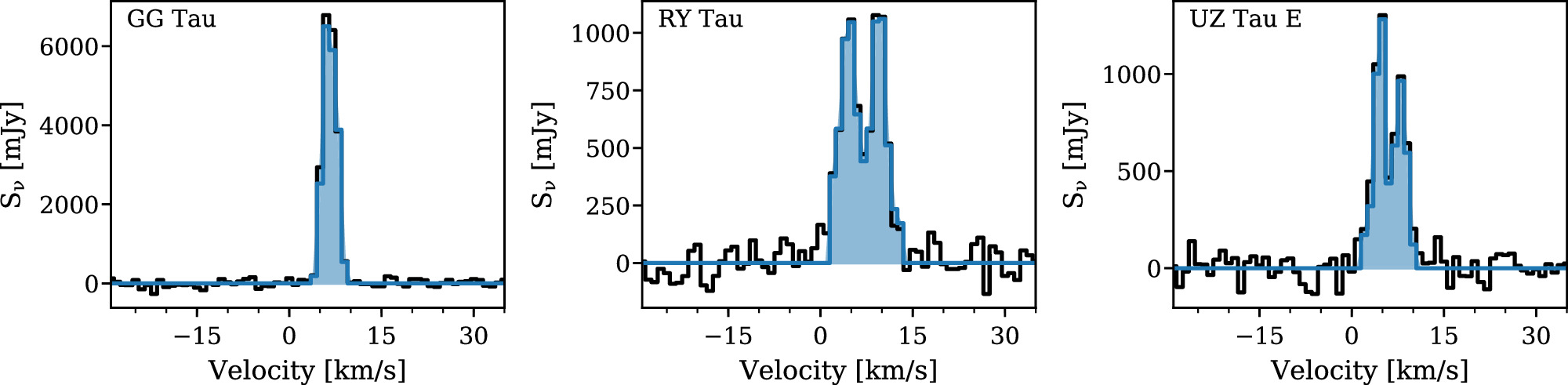
Figure 1. Spectra showing 13CO, C18O (J = 3–2 for the top three rows, 2–1 for the bottom four), HCO+, HCN, and N2H+ (J = 3–2) line emission from the observed disks described in Sections 2.1–2.2. Black curves show the integrated flux from within the channel-summed empirical mask, whereas the integrated fluxes within the channel-by-channel empirical masks are shown in blue (line detections) or red (nondetections). Empirical masks are based on bright line emission as described in Section 2.3.
Download figure:
Standard image High-resolution imageSpectra are generated by multiplying the final image by a specific mask using CASA's immath and producing a spectrum of the product using specflux. For the sufficiently bright and largely unresolved line emission in this work, the empirical masks based on the dirty images do not significantly differ from those derived from the clean images when using the same approach and remain appropriate for this step. The black lines in Figure 1 show spectra generated using a channel-summed version of each line's empirical mask over the entire image cube. The blue solid (for detections) and red dotted (for nondetections) lines show the flux collected in each individual channel of the original (non-channel-summed) empirical mask. The blue spectra are integrated over the line velocity range to produce the flux estimates given in Table 2. Noise estimates are determined by applying each line's empirical mask to 30 different line-free regions across the image cube. Because some of the selected line-free regions are off the phase center, the primary beam correction using CASA's impbcor was applied to the image before the noise and line flux estimates were made. The spatial regions sampled are selected to be as close to the source region as possible without sampling line emission to mitigate overestimation of the noise, which is dependent on the distance from the phase center. In our case, the primary beam correction had almost no effect on the line flux estimates. The standard deviation of fluxes from the 30 line-free regions is added in quadrature with 10% of the integrated line flux representing the assumed uncertainty for the flux amplitude calibration (Cortes et al. 2023) and provided as the uncertainties listed in Table 2. Upper limits are estimated as three times this uncertainty value with fluxes above this threshold being considered detections.
Table 2. Disk-integrated Molecular Line Fluxes
| Source Name | Line Fluxes (mJy km s−1) a | Ref. | |||||
|---|---|---|---|---|---|---|---|
| 13CO | C18O | HCO+ | HCN | N2H+ | |||
| 1 | J16142029–1906481 | 27.7 ± 3.0(1) | 7.5 ± 1.1(1) | 78.2 ± 8.1(1) | <8.4(1) | <5.8(1) | [1, 2, 3] |
| 7.5 ± 2.2(1)* | |||||||
| 2 | J16082324–1930009 | 30.7 ± 3.2(1) | 7.9 ± 1.5(1) | 62.8 ± 6.4(1) | 10.43 ± 1.07(2) | 18.9 ± 2.1(1) | [1, 2, 3, 4] |
| 11.8 ± 2.6(1)* | |||||||
| 3 | J16090075–1908526 | 39.9 ± 4.1(1) | 13.6 ± 1.8(1) | 57.0 ± 5.8(1) | 59.6 ± 6.2(1) | 10.2 ± 1.5(1) | [1, 2, 4] |
| 4 | RY Tau | 15.35 ± 2.89(2)* | <7.31(2)* | 13.58 ± 2.64(2) | 7.34 ± 1.76(2) | <5.45(2) | [1, 5] |
| 5 | UZ Tau Eab | 8.98 ± 2.16(2)* | <5.41(2)* | 7.73 ± 1.99(2) | <5.38(2) | <5.80(2) | [1, 5] |
| 6 | GG Tau A | 43.66 ± 5.20(2)* | 8.08 ± 2.11(2)* | 46.49 ± 5.33(2) | 24.45 ± 3.09(2) | 10.60 ± 2.40(2) | [1, 5] |
| 7 | IRAS 04302+2247 | 16.74 ± 1.75(3)* | 37.31 ± 4.90(2)* | 14.28 ± 1.45(3) | 23.12 ± 2.80(2) | 17.61 ± 2.20(2) | [1, 5] |
| 8 | Sz 65 | 9.71 ± 1.61(2) | 4.15 ± 1.13(2) | 21.9 ± 2.3(1) | <3.2(1) | <1.9(1) | [6, 7, 8] |
| <1.03(2)* | <6.0(1)* | ||||||
| 9 | Sz 130 | 47.0 ± 8.5(1) | <1.18(2) | 18.4 ± 2.0(1) | <3.7(1) | <2.7(1) | [6, 7, 8] |
| <9.6(1)* | <5.1(1)* | ||||||
| 10 | Sz 68 | 9.15 ± 1.61(2) | 4.44 ± 1.39(2) | 18.3 ± 2.0(1) | <2.4(1) | <1.5(1) | [6, 7, 8] |
| <1.21(2)* | <6.9(1)* | ||||||
| 11 | Sz 90 | 4.33 ± 1.07(2) | <1.84(2) | 29.8 ± 3.1(1) | 16.9 ± 2.6(1) | 7.0 ± 1.0(1) | [6, 7, 8] |
| <7.8(1)* | <5.4(1)* | ||||||
| 12 | J16085324–3914401 | 26.7 ± 5.3(1) | <1.36(2) | 25.4 ± 2.6(1) | 16.2 ± 1.9(1) | <3.6(1) | [6, 7, 8] |
| <7.5(1)* | <5.7(1)* | ||||||
| 13 | Sz 118 | 6.95 ± 1.50(2) | <2.36(2) | 37.6 ± 3.8(1) | 17.5 ± 2.1(1) | 6.4 ± 1.1(1) | [6, 7, 8] |
| 8.0 ± 2.7(1)* | <5.1(1)* | ||||||
| 14 | Sz 129 | 51.6 ± 8.9(1) | <1.09(2) | 59.5 ± 6.1(1) | 44.3 ± 4.6(1) | 20.3 ± 2.7(1) | [6, 7, 8] |
| <6.3(1)* | <4.8(1)* | ||||||
| 15 | IM Lup | 11.5 ± 1.7(3) | 27 ± 4(2) | 9.67 ± 1.01(3) | 56.54 ± 5.70(2) | 20.40 ± 2.10(2) | [9, 10, 11, 12, 13] |
| 83.70 ± 8.41(2)* | 15.92 ± 1.70(2)* | ||||||
| 16 | DM Tau | 30 ± 3(2) | 52.3 ± 5.4(2) | 29.66 ± 4.00(2) | 12.86 ± 1.35(2) | [11, 13, 14, 15, 16] | |
| 6.84 ± 1.04(3)* | 11.16 ± 1.10(2)* | ||||||
| 17 | GM Aur | 50.28 ± 5.05(2)* | 10.92 ± 1.16(2)* | 43.7 ± 4.7(2) | 18.35 ± 2.12(2) | 14.87 ± 1.50(2) | [10, 11, 16] |
| 18 | AS 209 | 22.69 ± 2.30(2)* | 53.8 ± 6.0(1)* | 40.2 ± 4.3(2) | 37.07 ± 3.80(2) | 91.7 ± 9.3(1) | [10, 11, 12, 13] |
| 19 | TW Hya | 46.1 ± 4.6(2) | 12.1 ± 1.2(2) | 12.9 ± 2.1(3) | 8.5 ± 1.7(3) | 20.0 ± 2.1(2) | [15, 17, 18] |
| 27.6 ± 1.8(2)* | 57 ± 6(1)* | ||||||
| 20 | V4046 Sgr | 84.4 ± 9.6(2)* | 12.03 ± 1.20(2)* | 11.43 ± 1.17(3) | 10.000 ± 1.000(3) | 37.61 ± 3.85(2) | [11, 12, 13, 19] |
Notes.
a In this table, flux values (i ± j) × 10k are abbreviated as i ± j(k). Fluxes are reported for the J = 3–2 transition, except for the 13CO and C18O J = 2–1 fluxes indicated with an asterisk (*). Line flux values are listed here at the source distance but scaled to a common distance of 160 pc prior to further comparison analyses.References: [1] This work, as described in Section 2.3; [2] ALMA 2018.1.01623.S; [3] Bergner et al. (2020); [4] ALMA 2015.1.01199.S; [5] SMA 2018B-S046; [6] Ansdell et al. (2016); [7] Ansdell et al. (2018); [8] Anderson et al. (2022); [9] Cleeves et al. (2016); [10] Öberg et al. (2021); [11] Qi et al. (2019); [12] Öberg et al. (2011); [13] Bergner et al. (2019); [14] Guilloteau et al. (2013); [15] Zhang et al. (2019); [16] Guilloteau et al. (2016); [17] Cleeves et al. (2015); [18] Trapmanet al. (2022); and [19] Kastner et al. (2018).
Download table as: ASCIITypeset image
2.4. Data from the Literature
Our analysis combines the observations described above with data from the literature. Here we describe the literature data that have been included. Available source distances are from Manara et al. (2022), which are derived by inverting their parallaxes from Gaia Data Release 3 (Gaia Collaboration et al. 2021). The values for AS 209, TW Hya, and V4046 Sgr (which are not included in Manara et al. 2022) are derived in the same manner. For IRAS 04302+2247, the distance is taken to be 161 pc (Garufi et al. 2021). Most sources belong to the Lupus (≲3 Myr), Taurus (∼1–3 Myr), and Upper Sco (∼5–10 Myr) star-forming regions (Manara et al. 2022). AS 209 resides to the northeast of the main Ophiuchus region in Oph N 3a, with an estimated age ∼1 (0.4–2.5) Myr (Andrews et al. 2018). TW Hya and V4046 Sgr are located in the nearby TWA (∼8 Myr) and β Pic MG (∼24 Myr), respectively (Kastner & Principe 2022).
Dust masses (Table 1) are computed as described in Manara et al. (2022) with the formula used by Ansdell et al. (2016) from Hildebrand (1983):

where κν = 2.3(ν/230 GHz) cm2 g−1 and assuming a dust temperature of 20 K. This assumes optically thin, isothermal dust emission at (sub-)millimeter wavelengths. The submillimeter dust emission may in fact be optically thick (e.g., Zhu et al. 2019; Sierra et al. 2021; Xin et al. 2023), resulting in higher dust masses and complicating our search for trends in this analysis since we would not be tracking the true dust mass. Continuum fluxes from Manara et al. (2022) are used when available. In addition, the continuum flux data from the following works are included: Andrews et al. (2018) for AS 209, van't Hoff et al. (2020) for IRAS 04302+2247, Tsukagoshi et al. (2016) for TW Hya, and Kastner et al. (2018) for V4046 Sgr. The selected continuum fluxes used here are those measured at frequencies of 225–240 GHz, with the exception of Upper Sco for which the continuum fluxes were measured at 340.7 GHz. The uncertainty in the dust mass (see the error bars in Figure 2) is taken as a 10% systematic uncertainty in the flux amplitude calibration (e.g., Andrews et al. 2013, 2018) converted into a mass value using the formula above.

Figure 2. N2H+, HCN, HCO+, and C18O J = 3–2 observed line fluxes (columns) compared to disk dust masses (first row). The line fluxes are also normalized by the dust mass (second row) or C18O line flux (third row). The fluxes are scaled to a distance of 160 pc. The arrows represent upper or lower limits. The colors indicate the source or star-forming region as shown by the key in the bottom right. Computed correlation coefficients are provided in the upper left of each panel. Correlation coefficients are not provided for the final row because there are no upper or lower bounds on the flux ratios. See the discussion of this figure in Section 3.2.1.
Download figure:
Standard image High-resolution imageThe ALMA observations of GG Tau A by Akeson et al. (2019) result in a dust mass ∼ 4 M⊕ for the circumstellar disk around GG Tau Aa. At their high angular resolution (with a beam of 0 18 × 016), they are able to separate the circumstellar emission from the wider ring around the GG Tau A multiple system. Given that our line flux observations of GG Tau A were taken at a lower angular resolution and we do not separate out these different components, we use the larger continuum flux value measured by Andrews et al. (2013) for the dust mass (∼277 M⊕) in our analyses.
Spectral types, stellar luminosities, stellar masses, mass accretion rates, and millimeter dust disk sizes (based on the radius enclosing 68% of the total continuum flux, Rcont,68) are taken from Manara et al. (2022, and references therein) when available. See Table 1 for additional references used for data on AS 209, TW Hya, and V4046 Sgr. Also note that Sz 68, GG Tau A, UZ Tau E, and V4046 Sgr are all binary or multiple-star systems, which may complicate the interpretation of their data and behavior relative to single stars.
Line fluxes are taken from the literature referenced in Table 2. In cases where multiple literature values were available, higher sensitivity observations with stronger signals in the observed spectra are preferred. When multiple analyses were performed on the same or similar data sets, the value derived using the Keplerian mask approach is used. Most fluxes derived from data sets with similar sensitivities are consistent across the different methods used in the literature, but a few varied by up to ∼2× (e.g., HCN in IM Lup and C18O J = 2–1 in V4046 Sgr). The uncertainty values listed in Table 2 include flux calibration uncertainties of 10%–15% as specified in the literature referenced in the final column of the table (this systematic uncertainty was added in quadrature to previously reported uncertainties if not already included).
The fluxes shown in the analyses in this work (Section 3) are for the J = 3–2 transition for each molecule. When only 13CO and C18O J = 2–1 fluxes are available, they are multiplied by a factor of 2× as a conversion to approximate the J = 3–2 fluxes. The accurate value for this conversion is uncertain. For optically thin emission in local thermodynamic equilibrium (LTE), this conversion would be ∼4–5× for 20–30 K gas. We base our value on the observed ratios of C18O (3–2)/(2–1) that are available for three sources in our sample. These values are in the range of ∼1–3, not well described by an optically thin LTE analysis. The line fluxes in the following analyses (Section 3) are corrected for differences in source distances by scaling to a uniform distance of 160 pc.
3. Results
Using the newly measured line fluxes in combination with preexisting data from the literature, we search for any relationships among the physical and chemical source properties. Our sample includes a maximum of 20 sources per comparison (based on the availability of data, see Table 1) across different star-forming regions. Five sources—three from Upper Sco, TW Hya, and V4046 Sgr—are >5 Myr old, representing a later stage of disk evolution relative to the 15 younger disks (1–3 Myr old) in our sample.
3.1. Line Detections from New Observations
First, we present the disk-integrated line fluxes measured using the method described in Section 2.3 for sources 1–7 in Table 2. Figures 1 and A1 show the spectra and velocity-integrated line intensity (moment 0) maps, respectively, for all seven sources. We detected N2H+ in IRAS 04302+2247 and GG Tau A, in addition to the previously identified N2H+ emission in two of the Upper Sco sources (Anderson et al. 2019). HCO+ is detected in all seven sources, while HCN is detected in five. 13CO and C18O are both detected in all three Upper Sco disks. 13CO is detected in all four of the Taurus disks, but C18O is only clearly detected in two. Note that the differences in the detection rates between the Upper Sco and Taurus samples are due to the difference in requested sensitivity of the observations for each survey (see Sections 2.1–2.2). For the Taurus disks, the main isotopologue of CO is also detected in all four disks (see Figure A2). Additional molecules detected but not discussed in this work are CN in all three Upper Sco disks and C2H and H2CO in GG Tau A.
3.2. Searching for Line Flux Trends
With the combined list of newly measured disk-integrated line fluxes and those from the literature, we search for any relationships between the line fluxes (or flux ratios) and other observed stellar and disk properties. The references for the stellar and disk properties used in this analysis are provided in Table 1 and Section 2.4. To provide an appropriate comparison of the flux values, fluxes are scaled to a common distance of 160 pc for these analyses. Fluxes are multiplied by where d is the source distance in parsecs from Table 1. Using the Python linear regression tool linmix 12 based on the method of Kelly (2007), we test for linear correlations between pairs of parameters. Kelly (2007) produced a Bayesian method that takes into account measurement errors in two variables and nondetections in one variable in linear regression. We apply this method to investigate trends with fluxes and normalized fluxes where we have nondetections in one variable. The method uses Markov Chain Monte Carlo sampling to approximate the posterior distribution. The computed linear correlation coefficient ranges from −1 for a strong negative correlation to 1 for a strong positive correlation, with a value of zero indicating no correlation between the two variables. We report the median correlation coefficient from the linmix runs with one standard deviation as the listed uncertainties. A summary of the computed correlation coefficients is provided in Figure A5.

3.2.1. Line Fluxes versus Dust Mass
The (sub-)millimeter dust mass provides an indication of the amount of solid material present in the disk. Meanwhile, the four molecular tracers track different components of the disk gas. By comparing these line fluxes with the disk dust masses we can investigate whether these various gas components and the dust are related or independent. Note that these trends may be affected by the optical thickness of the dust and/or line emission. 13CO and HCO+ are expected to be the most abundant of the selected species and the most likely to be optically thick, although in sufficiently bright sources emission from other molecular species may be optically thick as well. Bergner et al. (2019) find HCN J = 3–2 emission to be optically thick in AS 209 and V4046 Sgr based on the H13CN/HCN ratio. Here we choose to make comparisons with C18O rather than 13CO because while both trace the CO abundance, the rarer isotopologue C18O is expected to be less effected by optical depth effects. Anderson et al. (2022) found no trend between the line fluxes and dust masses of seven disks in Lupus (numbered 8–14 in Table 2). In the present larger sample, the top row of Figure 2 shows that the line fluxes of all four molecular species generally increase with the disk dust mass. This is consistent with the idea that disks with more dust have more material overall and therefore stronger molecular emission.
There appears to be a change to a steeper slope in line flux versus dust mass for disks with more than ∼10–100 M⊕ mass in dust. While this is particularly apparent in the HCO+ emission, whether the same trend exists for N2H+, HCN, and C18O is ambiguous given the current nondetections. The canonical mass of solid material needed to initiate runaway gas accretion leading to giant planet formation is ∼10 M⊕ (although it depends on disk parameters as shown by Piso & Youdin 2014). This break in the line emission versus dust mass could indicate a difference in the gas-to-dust mass ratio between systems that currently have enough solid material to undergo future gas giant planet formation versus those that do not. Disks with <10 M⊕ of solids may have already undergone giant planet formation or they may have never contained sufficient solid material to allow for giant planet formation from their onset. The apparent change in slope could alternatively be the result of the transition from optically thin to optically thick emission, where line fluxes transition from tracking the column density of molecular gas to the gas temperature. As the molecular gas column of a species increases, it increases the likelihood of its emission becoming optically thick. We expect this transition to occur within the set of observed fluxes, but deriving the exact location for each molecular transition would require more knowledge of the individual physical disk structures. In addition, assuming the correlation between the molecular gas column densities and Mdust is stronger than the correlation between the emitting layer gas temperatures and Mdust, one would expect the optically thin emission to have a stronger positive correlation with Mdust than the optically thick emission. The trend seen in Figure 2 defies this expectation.
For N2H+, HCN, and C18O, the significance of the increasing trends in molecular line fluxes with Mdust is affected by several upper limits in the measured line fluxes. The median correlation coefficients indicate a tentative to moderately significant positive linear correlation between the molecular fluxes and Mdust for all four molecular species. Computed correlation coefficients are listed in the upper left-hand corner of the individual panels in Figure 2.
When molecular fluxes are normalized by Mdust (Figure 2, row 2), they show a relatively flat trend with 2 or more orders of magnitude in scatter relative to Mdust. The flat trend suggests that within the limits of this sample there are no differences in the Mdust-normalized line flux ratios between disks with smaller versus larger dust masses. Worthy of note, there is no clear change in the normalized line flux indicating where the transition from optically thin to optically thick line emission might occur. Moreover, the large scatter in the dust-normalized line fluxes suggests that while the line fluxes have some dependence on Mdust, there are still other factors that control these molecular line fluxes.
To search for potential variations in the chemical composition of the disk gas versus Mdust, we examine the line flux ratios of N2H+, HCN, and HCO+ over the C18O line flux. Sources are excluded from the plot when neither species in the ratio is detected. Here we generally find a flat trend with scatter ranging more than 2 orders of magnitude, revealing no clear distinctions in gas-phase chemical abundances as a function of changing dust mass (as indicated by molecular line fluxes), but rather a large amount of variation across the whole dust mass range.
3.2.2. Line Fluxes versus Other Stellar and Disk Properties
In addition to the disk dust mass comparison, we also compared the molecular fluxes to other observed source properties from the literature. Through these comparisons we can investigate which source properties are influencing the chemical behavior of the disk and determine disk-integrated molecular fluxes. Data are plotted based on availability, thus not all panels contain the full 20 disks in the sample. Error bars are not included for the following parameters: Mstar, Lstar, Macc, or Rcont,68. See Manara et al. (2022) for discussion on the uncertainties involved in acquiring these values.
Anderson et al. (2022) found no trends with stellar mass or luminosity. Our larger sample yields similar results (Figure 3, columns (1)–(2)). As shown in the Appendix, Figure A3, normalizing the molecular line fluxes by Mdust results in a partially decreasing trend with stellar mass and luminosity but the median correlation coefficients are not more than 1–2 standard deviations above zero. This is most noticeable for HCO+. The molecular fluxes show generally increasing trends with the mass accretion rate, similar to their behavior with dust mass (Figure 3, column (3)). This is expected given the known relationship between the mass accretion rates and dust masses of protoplanetary disks (Manara et al. 2016; Mulders et al. 2017; Manara et al. 2020). However, given the smaller number of data points and some additional scatter, the linear correlation coefficients are less significantly different from zero. When normalizing the molecular line fluxes by Mdust or the C18O flux, there are no significant trends with Macc (see the Appendix, Figure A3).

Figure 3. N2H+, HCN, HCO+, and C18O J = 3–2 observed line fluxes (rows) compared to stellar masses (first column), stellar luminosities (second column), mass accretion rates (third column), and outer disk radii seen in (sub-)millimeter dust (fourth column). The fluxes are scaled to a distance of 160 pc. The arrows represent upper limits. The colors indicate the source or star-forming region as indicated in Figure 2. Only a subset of the sample is shown per panel as literature data were not equally available for all sources (see Table 1). Computed correlation coefficients are provided in the upper right of each panel. See the discussion of this figure in Section 3.2.2.
Download figure:
Standard image High-resolution imageSimilar to the behavior with Mdust, molecular fluxes for all four species generally increase with the outer radius of the (sub-)millimeter dust disk (Figure 3, column (4)). This is consistent with the idea that larger disks have more gaseous material and therefore stronger molecular line emission. However, where line emission becomes optically thick this could also be a trend in disk temperature. Perhaps larger disks have more material, pushing emitting regions of optically thick lines to the hotter layers closer to the disk surface. The median correlation coefficients show positive linear correlations between the molecular fluxes and Rcont,68. When normalizing the molecular line fluxes by Mdust or the C18O flux, there are no significant trends with Rcont,68 (see the Appendix, Figure A3).
3.2.3. Comparison among Line Fluxes
To investigate potential chemical links between molecular species, we compare pairs of molecular line fluxes from different species against each other in Figure 4. Anderson et al. (2022) found a tentative positive correlation among N2H+, HCN, and HCO+ fluxes in their set of Lupus sources (8–14 in Table 2). These molecular fluxes were not correlated with their 13CO J = 3–2 fluxes. Limited C18O detections across their sample prevented a comparison with C18O. In this sample of 20 sources, we find at least a tentative positive correlation in fluxes for all pairs of molecular species. The correlation coefficients computed using linmix (excluding any cases where both line fluxes are upper limits) show strong positive correlations between all combinations of 13CO, C18O, HCO+, and N2H+. For HCN, we find strong positive correlations with HCO+ and N2H+ and tentative positive correlations with 13CO and C18O. Correlation coefficients are provided in Figure 4. But some of these strong correlations may break down for fainter line fluxes where constraints are lacking due to the observational bias toward brighter disks.

Figure 4. N2H+, HCN, HCO+, 13CO, and C18O J = 3–2 observed line fluxes compared to each other. The fluxes are scaled to a distance of 160 pc. The arrows represent upper limits in either direction. The colors indicate the source or star-forming region as shown by the key in the bottom right. Computed correlation coefficients are listed in the upper left of each panel. Values listed in gray are based on only a subset of the sample, limited to sources where one or both of the fluxes values were detected. See the discussion of this figure in Section 3.2.3.
Download figure:
Standard image High-resolution imageCorrelations could be driven by physical or chemical relationships between the molecular species, or more likely, a combination of both. The strong correlation between 13CO and C18O is unsurprising because they both track the same underlying CO abundance. In other cases, chemistry can provide explanations for positive correlations between some pairs of molecular species: CO is a precursor to the formation of HCO+, while N2H+ and HCN are both carriers of N. However, the chemical relationship between N2H+ and CO, where N2H+ is readily destroyed when CO is abundant (Qi et al. 2013), would suggest they should be anticorrelated. This might be an indicator that physical disk properties, such as gas mass or temperature, are playing a larger role in determining these disk-integrated molecular fluxes. The level of ionization in the disks may also be an important factor, in particular for the fluxes of molecular ions N2H+ and HCO+.
The optical thickness of the line emission is another important factor to consider. The molecular line flux correlations generally appear less strong at lower flux values, below ≲1 Jy km s−1 at a distance of 160 pc. This could be a sign of diverging pathways of chemical evolution and gas-phase chemical abundances among the fainter (typically smaller and less massive, see Figures 2–3) disks. Alternatively, the change could represent the transition from optically thin to thick line emission, where optically thick emission is mainly tracking the gas temperature rather than the molecular column density. This would also indicate a correlation in the gas temperatures within the emitting layer of different molecular species. Isotopologue ratios (e.g., 13CO/C18O and HCN/H13CN) have revealed that emission from 13CO and the dominant isotologues of other molecular carriers are optically thick in a number of protoplanetary disks (e.g., Schwarz et al. 2016; Bergner et al. 2019).
Figure 5 compares the fluxes of all four molecular species (N2H+, HCN, HCO+, and C18O) against each other to give a more complete view of the variations in chemical tracers in each disk. Given the strong correlation between 13CO and C18O, only C18O is included to simplify the plot. HCO+ makes up around 35%–55% of the total molecular flux. It is generally the largest flux contributor of the four molecular species, with the exception of the C18O-dominant disks Sz 68 and Sz 65 and the HCN-dominant disks J1608 and J1609. The relative HCO+ flux is particularly high in J1614, making up more than 80% of the total molecular flux. The spectral shape of the HCO+ flux is also an anomaly in this data set (see Figure 1), suggesting special circumstances in this case. Perhaps this disk is displaying an outflow or temporary flare in HCO+ emission (Cleeves et al. 2017; Waggoner & Cleeves 2022).

Figure 5. Relative comparison of the N2H+, C18O, HCN, and HCO+ J = 3–2 observed line fluxes for each source. Line fluxes (labeled along the right-hand side) are plotted as fractions of the total flux, where the total flux is the sum of the four line fluxes. Hatched shading indicates upper limits on the fractions of nondetected lines. Sources are separated by star-forming region and age as shown by the labels along the top of the figure. See the discussion of this figure in Section 3.2.3.
Download figure:
Standard image High-resolution imageThe relative HCN flux is highly variable, ranging from less than a few to over 40% of the total molecular flux. It is generally higher in disks where the fraction of C18O flux is low. The relative C18O flux also spans a large range of values from less than a few to over 60% of the total molecular flux. The disks with the largest C18O fractions belong to younger star-forming regions: Taurus, Lupus, and Oph (left side of Figure 5). But overall, the fraction of C18O is variable across the younger disks. In contrast, the C18O fractions are all <10% in the older disks (rightmost five disks in Figure 5). Across all sources, N2H+ makes up less than 15% of the total molecular flux. The lowest N2H+ fractions are less than a few percent, but upper limits prevent us from determining the full range and any additional patterns in N2H+ fractions. For at least the cases of Lupus and Upper Sco, disks from the same star-forming region display different relative fractions of molecular fluxes. This may be indicative of a range of gas chemical compositions coexisting within a single star-forming region.
3.3. Disk Gas Masses
The total disk gas mass is an essential parameter regulating planet formation mechanisms and the number of planets that can form in a given system. Disk masses are dominated by H2 gas, which is unobservable at cold temperatures throughout the bulk of the disk. As such, indirect tracers, most often submillimeter dust and CO isotopologue emission, are traditionally used to provide disk gas mass estimates. While both are readily observable and useful for a first look, the accuracy of the resulting gas mass estimates ultimately depends on the accuracy of the gas/dust or CO/H2 conversion factor. The dust may evolve separately from the gas over time, resulting in uncertainty in the gas/dust ratio. CO/H2 can also vary spatially and temporally within the disk and among different systems (e.g., Schwarz et al. 2016; Zhang et al. 2019, 2021). Measuring CO/H2 values in protoplanetary disks requires at least one additional measured quantity beyond CO isotopologue emission, preferably one that is tied to the H2 content of the gas. Hydrogen deuteride (HD) measurements enabled by the Herschel Space Observatory (Bergin et al. 2013; McClure et al. 2016) revealed CO/H2 up to 100× below the typically assumed interstellar value ∼10−4 in a few protoplanetary disks. Since the end of Herschel's mission, there have not been any observatories equipped for the necessary HD measurements. Meanwhile, developments have been made in using N2H+ in combination with CO to provide constraints on both the CO/H2 and H2 mass (Anderson et al. 2019, 2022; Trapmanet al. 2022). N2H+ is readily observable by ground-based radio observatories including ALMA and the SMA.
We use our data to compare disk gas mass estimates based on measurements of (sub-)millimeter dust, CO gas, and from combinations of molecular gas tracers. In Figure 6, we plot an initial look at how disk gas masses vary with age across our selected sample. The top panel shows gas masses as equal to 100 × Mdust. Dust masses are computed using (sub-)millimeter continuum emission as described in Section 2.4. More than half of this sample lie above 0.01 M⊙, with the remaining sources extending to values 1–2 orders of magnitude lower. The Lupus sources represent values across the full range, whereas the Taurus sources and Upper Sco sources are each grouped around a narrower range of disk dust mass values. Previous comparisons across star-forming regions find decreasing median dust masses with age (e.g., Ansdell et al. 2017; Cieza et al. 2019; Villenave et al. 2021). The sources in this sample were not selected to be representative of the population in their respective star-forming regions. Selection is often biased toward brighter sources, therefore this comparison is not representative of typical sources across the star-forming regions included in this work.

Figure 6. Disk mass vs. age for disk gas masses estimated using 100× the dust mass (top), fit functions from the models of Miotello et al. (2016, 2017) with available observed 13CO and/or C18O fluxes (middle), and an approximation based on the N2H+/C18O flux ratio (bottom). The limits in the bottom panel (shown in black) are based on HD from Trapmanet al. (2022). The colors indicate the source or star-forming region as indicated in the top panel. See Section 3.3 for details on the mass estimates and Section 2.4 for age references.
Download figure:
Standard image High-resolution imageThe second panel in Figure 6 shows gas masses based on CO isotopologue observations. These masses were computed using the fits functions provided by Miotello et al. (2016, 2017) from their large grid of models. Masses were based on C18O fluxes from either the J = 3–2 or J = 2–1 transitions using the appropriate functions for each from Miotello et al. (2016, 2017). Where fluxes for both transitions are available, the one with a higher signal-to-noise ratio was used. For sources where C18O has not been detected, 13CO fluxes and appropriate functions are used instead. With the exception of the young source IRAS 04302+2247, the CO-based gas masses are lower than the dust-based values by roughly 1–2 orders of magnitude. While IRAS 04302+2247 is part of the Taurus star-forming region and that age is used here, it may represent an earlier evolutionary stage as it is classified as a Class I source (Lucas & Roche 1997; Garufi et al. 2021). The distinction between gas masses derived from (sub-)millimeter dust and those derived from CO isotopologues is well documented in large-population ALMA studies of multiple star-forming regions (e.g., Ansdell et al. 2016; Long et al. 2017; Miotello et al. 2017). As discussed in these previous works, the differences between the gas mass estimates derived from these two methods could be the result of gas/dust ratios and/or CO/H2 abundances decreasing over time as the disks evolve.
Anderson et al. (2019, 2022) and Trapmanet al. (2022) have shown that by using a combination of N2H+ and CO observations, we can place constraints on both the total disk gas mass and CO/H2. In this way, we can distinguish between the effects of depleted gas/dust ratios versus depleted CO/H2. The extensive modeling analysis needed to constrain CO/H2 and H2 masses for this sample of disks is beyond the scope of this work. But to give a rough idea of how this might affect our inferred gas masses, we perform a simple scaling of the CO-based total H2 gas masses from the middle panel of Figure 6. These values assume a CO/H2 abundance ∼ 10−4. We increase these values by a factor corresponding to the CO/H2 abundances derived from the observed N2H+/C18O flux ratios for each source. For CO/H2, we used the modeled relation between the N2H+ (3–2)/C18O (2–1) flux ratio and the CO/H2 abundance for the TW Hya model with a cosmic-ray ionization rate of 10−18 s−1 from Trapmanet al. (2022). In reality, this relation will depend on the individual physical/chemical structure of each disk (Trapmanet al. 2022) and further exploration of how much this relation varies over a wider parameter space is needed.
Based on this approximation, the gas masses for a subset of our sample were increased by factors ∼5–135 relative to the CO-based values. Some disks have N2H+/C18O flux ratios that are consistent with a CO/H2 of 10−4, including disks where only an upper limit on this flux ratio is available, so their gas mass estimates were not changed from the CO-based values. The gas mass value for IRAS 04302+2247 was also not increased given its already high value. The final result is a larger spread in the range of gas masses for each age group (Figure 6, bottom panel). The additional constraints on CO/H2 increase the gas mass estimates for some disks to values that are closer to the dust-based masses (Figure 6, top panel). The mass estimates based on HD emission (Bergin et al. 2013; McClure et al. 2016; Trapmanet al. 2022) also suggest that the CO-based values are underestimating the total amount of H2 gas present. Our conclusions are limited by the size of and selection biases present in the current sample. Ultimately, more data are needed to explore the evolution of disk gas masses, especially data from older sources (ages > 5 Myr).
4. Discussion
4.1. Comparison within Our Sample
This data set includes 20 disks spread across various birth environments and ages. Within this sample, we find examples of disks with very different disk-integrated molecular flux ratios, even for disks residing in the same star-forming region. In Figures 2–3 color is used to distinguish sources from different star-forming regions or moving groups. In this case, any apparent disparities among disks from different star-forming regions are likely caused by differences in the sample selection criteria used for the different sets of observations. As a result, the selected Taurus and individual sources (AS 209, TW Hya, and V4046 Sgr) tend to have larger and brighter disks relative to those from Lupus and Upper Sco. When normalized by Mdust or C18O, the molecular fluxes fall within generally the same range within 1–2 orders of magnitude regardless of star-forming region—with a few exceptions. There are two sources from Lupus (Sz 65 and Sz 68, both appearing as upper limits in Figures A3–A4) for which constraints on the normalized N2H+ and HCN values fall well below the rest of the sample. This could be an indication that these two sources have a distinct disk gas chemical composition from the others.
For the comparisons made in Figures 2–4, we see no obvious distinctions between the younger sources (the AS 209, Taurus, and Lupus disks; 1–3 Myr old) and the older sources (the Upper Sco, TW Hya, and V4046 Sgr disks; >5 Myr old). Although, for at least 4/5 of the older sources, their N2H+, HCN, and HCO+ fluxes normalized by Mdust or C18O are among the highest values in the sample. There are hints of more uniformity among these disks (Figure 5). The fifth source, J1614, stands out by having a relatively large amount of HCO+ emission with an unusual line shape. However, even when excluding HCO+, J1614 still differs from the other >5 Myr old sources due to its low HCN/C18O flux ratio.
It should be noted that different age ranges are not uniformly sampled in this work. The older populations may suffer the greatest selection bias, often toward brighter objects that still have molecular gas. Overall, aged populations are more poorly sampled in multimolecular observations. Furthermore, this comparison may be muddled by uncertainty in the individual source ages and potential age variations within the star-forming regions (e.g., Krolikowski et al. 2021). A more uniform unbiased survey of disks across different age brackets is needed to investigate fully the trends in the molecular fluxes with disk age.
Sample bias and incompleteness largely affect this current analysis. The selected sources tend to be among the largest and brightest in their respective star-forming regions. The star-forming regions included in this comparison are also not equally sampled, with fewer sources particularly for the older populations. Furthermore, because the sample is compiled from different observing programs, the sensitivity is not the same for all sources or molecular lines. Additional uncertainty is introduced when trying to make comparisons using different transitions of CO isotopologues (see Section 2.4). Current ALMA Large Programs in progress, namely AGE-PRO: The ALMA Survey of Gas Evolution in PROtoplanetary Disks and The ALMA Disk-Exoplanet C/Onnection (ALMA DECO), will provide a more uniform sampling and analysis of multiple molecular lines across different star-forming regions.
Within our sample are four systems that contain multiple stars. Given the current data set, there are no obvious flux trends that set these systems apart from the single star systems. Although it should be noted that the data sets of stellar and disk properties are not complete for our sample, especially for the stellar multiple systems. In addition, using spatially resolved observations that can distinguish between different disk components in these complex systems (e.g., disks around individual stars versus disks around binaries) may be necessary to make more meaningful comparisons.
There are many relevant parameters that could affect the observed molecular line fluxes that have not been explored in this work. This is largely due to limitations in the data readily available for this combined sample. Additional stellar properties such as UV and X-ray spectra, stellar activity, and magnetic field strength could be explored for connections in the future. Fluxes will also depend on the individual density and temperature distribution of each disk. Determining whether these physical conditions are relatively consistent across populations (or subgroups within populations) or are unique to each individual source is an important step in understanding disk evolution and planet-forming environments.
4.2. Comparison with Previous Molecular Disk Surveys
Previous works have explored surveys of disk-integrated molecular line fluxes for different samples of disks and molecular species. Pegues et al. (2023) find that molecular line fluxes generally increase with continuum fluxes across their sample of T Tauri and Herbig disks (stellar masses of 0.15–2.5 M⊙), consistent with our trends in line flux with Mdust. Our results agree with Pegues et al. (2021) in finding no correlation between the flux ratio of HCN/C18O and Mstar (Figure A4). Pegues et al. (2023) also show that HCO+/C18O flux ratios (when both species are detected) are relatively flat with continuum flux and stellar luminosity for their T Tauri sample, similar to our findings.
While we find positive correlations between the disk-integrated line fluxes of all our molecular species pairs, this is not always the case. van Terwisga et al. (2019) found that CN fluxes do not strongly correlate with 13CO in disks from the Lupus star-forming region. Furthermore, the CN fluxes do not strongly correlate with the submillimeter continuum fluxes. However, for a subset of the sample (Miotello et al. 2019) show a strong correlation between CN and C2H fluxes and between both species and the stellar luminosity. The abundances of CN and C2H are largely affected by photochemistry, which might explain their correlation.
With a diverse set of 14 disks across a range of ages, stellar masses, and stellar luminosities (including some overlap with our sample), Bergner et al. (2019) find no correlation between disk-integrated HCN and C18O fluxes when both are normalized to the continuum flux. Here we find only a tentative trend between the HCN and C18O fluxes relative to strong positive correlations between other molecular species. In contrast, Pegues et al. (2021) report a significant positive correlation between HCN and C18O fluxes, although the correlation is not as strong as those between other molecular species pairs (C2H and HCN, H2CO and HCN). In addition, they find a positive correlation between C18O and Mstar, whereas we find no correlation. The sample of Pegues et al. (2021) includes disks around five low-mass stars (0.14–0.23 M⊙) alongside solar-type T Tauri and Herbig Ae disks. In comparison, our sample is more concentrated toward stellar masses ∼ 0.5–1 M⊙ and does not include such low-mass stars (<0.25 M⊙). Current trends are determined with limited numbers of disks and line detections, thus more sensitive observations of larger and more diverse samples of disks are ultimately needed to explore these discrepancies as well as to verify existing trends.
4.3. Comparison with Physical/Chemical Disk Models
Molecular abundances are sensitive to various physical and chemical properties of protoplanetary disks (Öberg et al. 2023). Molecular emission is further sensitive to excitation conditions, predominately how the abundance distribution aligns with the disk temperature and density structures. Physical/chemical disk models have explored how the molecular fluxes of some of our observed species depend on various stellar and disk parameters. Miotello et al. (2016) show that disk-integrated 13CO and C18O fluxes are sensitive to the disk mass and outer radial extent. The modeling of Boyden & Eisner (2023) shows HCO+ J = 4–3 emission increases with the outer disk radius, but decreases with increasing stellar mass and disk dust mass. Fedele & Favre (2020) find HCN J = 4–3 emission is insensitive to changes in stellar and physical disk parameters, including the total stellar luminosity, but sensitive to elemental ratios of C/O (particularly as C/H is reduced) and N/H. But note that the J = 3–2 HCO+ and HCN transitions observed here have lower upper state energies and likely trace a colder and therefore deeper vertical layer of the disk. Anderson et al. (2022) show that 13CO, HCO+, HCN, and N2H+ J = 3–2 emission generally increase together for increasing gas/dust ratios, but diverge with volatile depletion (C/H and O/H). As C and O are removed, 13CO and HCO+ emission decreases, while HCN and N2H+ emission increases.
While our observed trends agree with some of the model results (e.g., increasing line emission with disk radius), direct comparison with existing model grids is difficult. All model results depend on the assumptions made about the interplay of different disk parameters, for example, the relationship between gas and dust components of the disk and between disk mass and outer radius. The assumed relationships may not be reflective of our observed sample of disks. While beyond the scope of this work, a model grid exploring N2H+, HCN, HCO+, C18O, and 13CO J = 3–2 emission across the parameter space relevant to the star and disk properties of this observed sample would aid in the interpretation of the trends we find.
5. Conclusion
In this work, we present observations of N2H+, HCN, HCO+, and CO isotopologues in four disks from the young Taurus star-forming region and three disks from the older Upper Sco star-forming region. Using data from the literature, we create a sample of 20 disks from multiple environments, including five sources at ≳5 Myr old. We compare the observed molecular line fluxes with stellar and disk properties from the literature to look for connections indicative of underlying physical and/or chemical disk properties. Overall, we find molecular line fluxes generally increase with (sub-)millimeter disk dust masses and outer radii. But there is a great deal of scatter within these relationships. Strong positive correlations exist among the line fluxes of different molecular species. However, scatter in these relations indicate that even for disks in a single star-forming region—presumably of similar age and birth environment—there are differences in the physical and/or chemical properties that affect the relative molecular line fluxes of N2H+, HCN, HCO+, and C18O.
This sample has been compiled from numerous separate observing programs. The lack of uniformity in source selection and observing parameters certainly affect our current results. Future observing campaigns aimed at producing more uniform surveys of multiple molecular species in large populations of protoplanetary disks are needed to provide a more complete analysis of the tentative relationships in observed disk properties investigated here.
Acknowledgments
We thank the anonymous referee for feedback and suggestions. D.E.A. acknowledges support from the Virginia Initiative on Cosmic Origins (VICO) Postdoctoral and Carnegie Postdoctoral Fellowships. L.I.C. gratefully acknowledges support from the David and Lucille Packard Foundation, the Virginia Space Grant Consortium, Johnson & Johnson's WiSTEM2D Award, and NSF AAG grant number AST-1910106. This paper makes use of the following ALMA data: ADS/JAO.ALMA#2015.1.01199.S, ADS/JAO.ALMA#2018.1.01623.S, and ADS/JAO.ALMA#2019.1.01135.S. ALMA is a partnership of ESO (representing its member states), NSF (USA) and NINS (Japan), together with NRC (Canada), MOST and ASIAA (Taiwan), and KASI (Republic of Korea), in cooperation with the Republic of Chile. The Joint ALMA Observatory is operated by ESO, AUI/NRAO, and NAOJ. This paper also makes use of data from Submillimeter Array project 2018B-S046. The Submillimeter Array is a joint project between the Smithsonian Astrophysical Observatory and the Academia Sinica Institute of Astronomy and Astrophysics, and is funded by the Smithsonian Institution and the Academia Sinica. This work has made use of data from the European Space Agency (ESA) mission Gaia (https://www.cosmos.esa.int/gaia), processed by the Gaia Data Processing and Analysis Consortium (DPAC; https://www.cosmos.esa.int/web/gaia/dpac/consortium). Funding for the DPAC has been provided by national institutions, in particular the institutions participating in the Gaia Multilateral Agreement.
Software: Astropy (Astropy Collaboration et al. 2013; Price-Whelan et al. 2018), CASA (McMullin et al. 2007), linmix (https://github.com/jmeyers314/linmix), Matplotlib (Hunter 2007), and Numpy (van der Walt et al. 2011).
Appendix
Here we present the spectral window settings for the ALMA observations in Table A1, the moment 0 maps of integrated flux from the observations described in Sections 2.1–2.2 in Figure A1, and the main CO isotopologue emission for observed Taurus sources in Figure A2. Additional figures are included to show further comparisons between observed line fluxes normalized by Mdust (Figure A3) and C18O line fluxes (Figure A4) and source properties. A summary of the median correlation coefficients from the linmix analyses of parameter pairs are also presented in Figure A5.

Figure A1. Moment 0 maps of integrated flux for 13CO, C18O (J = 3–2 for the top three rows, 2–1 for the bottom four), HCO+, HCN, and N2H+ (J = 3–2) line emission from the observed disks described in Sections 2.1–2.2. Fluxes are integrated over the velocity range of −5–15 km s−1 for Upper Sco sources (−15–20 km s−1 for HCO+ in J1614), 4–9 km s−1 for GG Tau A, 2–8 km s−1 for IRAS 04302+2247, 2–10 km s−1 for RY Tau, and 2–13 km s−1 for UZ Tau E. The velocity ranges are based on the observed line emission and the ranges are inclusive for 1 km s−1 channels. Overplotted contours indicate the summed empirical masks used to encapsulate regions containing potential line emission. Red contours indicate nondetections.
Download figure:
Standard image High-resolution image
Figure A2. Spectra showing CO J = 2–1 line emission from the observed disks described in Section 2.2. Black curves show the integrated flux from within the channel-summed empirical mask, whereas the integrated fluxes within the channel-by-channel empirical masks are shown in blue. This CO emission was used to generate the empirical masks for fainter lines in these sources. Integrated CO fluxes (computed as described in Section 2.3) are 19,547 ± 1985 mJy km s−1 for GG Tau A, 7679 ± 794 mJy km s−1 for RY Tau, and 5523 ± 584 mJy km s−1 for UZ Tau E. The CO spectrum for IRAS 04302+2247 shows signs of absorption and is not used in this analysis.
Download figure:
Standard image High-resolution image
Figure A3. Variation of Figure 3 showing line fluxes normalized by disk dust masses. Normalized N2H+, HCN, HCO+, and C18O J = 3–2 observed line fluxes relative to disk dust masses (rows) compared to stellar masses (first column), stellar luminosities (second column), mass accretion rates (third column), and outer disk radius seen in (sub-)millimeter dust (fourth column). The fluxes are scaled to a distance of 160 pc. The arrows represent upper limits. The colors indicate the source or star-forming region as indicated in Figure 2. Only a subset of the sample is shown per panel as literature data were not equally available for all sources (see Table 1). Computed correlation coefficients are provided in the upper right of each panel.
Download figure:
Standard image High-resolution image
Figure A4. Variation of Figure 3 showing line fluxes normalized by the C18O line flux. Normalized N2H+, HCN, and HCO+ J = 3–2 observed line fluxes relative to C18O (rows) compared to stellar masses (first column), stellar luminosities (second column), mass accretion rates (third column), and outer disk radius seen in (sub-)millimeter dust (fourth column). The fluxes are scaled to a distance of 160 pc. The arrows represent upper or lower limits. The colors indicate the source or star-forming region as indicated in Figure 2. Only a subset of the sample is shown per panel as literature data were not equally available for all sources (see Table 1). Correlation coefficients are not provided because there are no upper or lower bounds on the flux ratios.
Download figure:
Standard image High-resolution image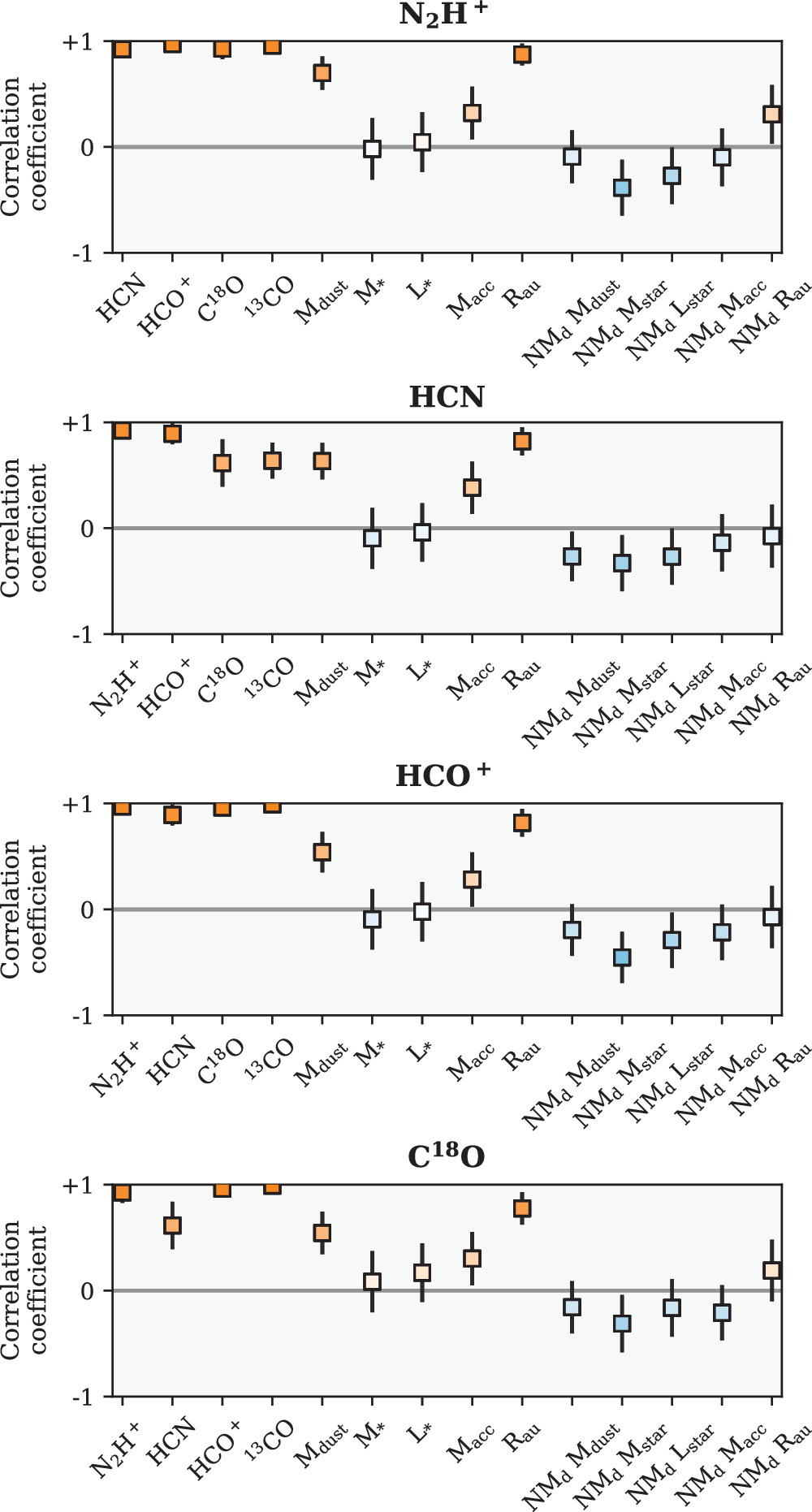
Figure A5. Median linear correlation coefficients for each source parameter (listed on the x-axis) with observed N2H+, HCN, HCO+, and C18O J = 3–2 fluxes. NMd denotes the molecular line fluxes normalized by Mdust (see Figures 2 and A3). Error bars represent one standard deviation in the linear correlation coefficients. Positive correlations (with coefficients from 0 to 1) are shown in orange and anticorrelations (0 to −1) in blue. Darker colors represent stronger (anti)correlations based on the median value. Values close to zero indicate no linear correlation between the two parameters.
Download figure:
Standard image High-resolution image
Table A1. Observational Settings
| Data Set | ALMA | Target | Spectral Windows | Beam Size | Int. a | ||
|---|---|---|---|---|---|---|---|
| Band | Width | Center | Channel | (min) | |||
| (GHz) | (Rest, GHz) | Width (kHz) | |||||
| 2015.1.01199.S | 7 | Spectral lines | 0.117 | 279.51176 (N2H+ J = 3–2) | 122.070 | ∼06 × 05 | 107 |
| Sources: J1608, J1609 | 281.52693 | ||||||
| 282.38109 | |||||||
| 282.92001 | |||||||
| 293.91209 | |||||||
| Continuum | 1.875 | 293.90000 | 976.562 | ||||
| 2018.1.01623.S | 6 | Spectral lines | 0.234 | 255.47939 | 244.141 | ∼04 × 04 | 23 |
| Sources: J1608, J1609 | 265.88643 (HCN J = 3–2) | ||||||
| J1614 | 267.55763 (HCO+ J = 3–2) | ||||||
| Continuum | 1.875 | 251.80000 | 976.562 | ||||
| 269.50000 | 15625.000 | ||||||
| 7 | Spectral lines | 0.469 | 279.51176 (N2H+ J = 3–2) | 244.141 | ∼04 × 04 | 36 | |
| 0.117 | 288.14386 | ||||||
| 289.20907 | |||||||
| 289.64491 | |||||||
| Continuum | 1.875 | 278.20000 | 15625.000 | ||||
| 291.05000 | |||||||
| 7 | Spectral lines | 0.234 | 329.33055 (C18O J = 3–2) | 244.141 | ∼08 × 06 | 57 | |
| 330.587967 (13CO J = 3–2) | |||||||
| 0.469 | 340.24777 (CN N = 3–2) | ||||||
| Continuum | 1.875 | 329.33055 | 976.562 | ||||
| 341.50000 | |||||||
Note.
a Approximate on-source time per source.Download table as: ASCIITypeset image
Footnotes
- 10
- 11
- 12