


Abstract
Magnetic flux emergence from the convection zone into the photosphere and beyond is a critical component of the behavior of large-scale solar magnetism. Flux rarely emerges amid field-free areas at the surface, but when it does, the interaction between the magnetism and plasma flows can be reliably explored. Prior ensemble studies have identified weak flows forming near emergence locations, but the low signal-to-noise ratio (S/N) required averaging over the entire data set, erasing information about variation across the sample. Here, we apply deep learning to achieve an improved S/N, enabling a case-by-case study. We find that these associated flows are dissimilar across instances of emergence and also occur frequently in the quiet convective background. Our analysis suggests the diminished influence of supergranular-scale convective flows and magnetic buoyancy on flux rise. Consistent with numerical evidence, we speculate that small-scale surface turbulence and/or deep convective processes play an outsized role in driving flux emergence.

Original content from this work may be used under the terms of the Creative Commons Attribution 4.0 licence. Any further distribution of this work must maintain attribution to the author(s) and the title of the work, journal citation and DOI.
1. Introduction
Active regions (ARs) are spatially and temporally extensive magnetic phenomena, extending from the solar interior to the corona, with a lifetime marked by formation, emergence, and eventual decay (van Driel-Gesztelyi & Green 2015) through dispersion of magnetic elements (Strous et al. 1996; Schunker et al. 2019, 2020) into the background turbulent convective field. Most ARs play host to sunspots (Rempel & Schlichenmaier 2011; Rempel 2012)—magnetic features characterized by evolving umbrae, penumbrae, and fine structures, with high field strengths (a few ∼kilogauss; Siu-Tapia et al. 2019). The dynamics of tangled magnetic field lines in morphologically complex ARs and sunspots underpin high-energy eruptive events, such as flares (Toriumi & Wang 2019) and coronal mass ejections (Webb & Howard 2012). A detailed inquiry into large-scale solar magnetism, vis-à-vis ARs, has indirect implications for understanding space weather (Temmer 2021).
ARs are hypothesized to be the surface manifestations of thin magnetic flux tubes (Cheung & Isobe 2014) generated in the interior (Charbonneau 2020), which then rise up (Birch et al. 2016) to the surface and above through a collection of processes termed emergence. The precise location of the dynamo is contested, with suggestions ranging from the base of the convection zone (Spiegel & Weiss 1980) to the near-surface layers (Brandenburg 2005). A comprehensive understanding of solar magnetism warrants that ARs be studied over the full domain—from birth to decay. Their associated flows have drawn attention (Gizon et al. 2001; Komm et al. 2008; Hindman et al. 2009), since magnetic fields and solar convection are thought to be intertwined (Stein 2012). A medley of findings, courtesy of individual emerging-active-region (EAR) studies (Komm et al. 2008; Zharkov & Thompson 2008; Kosovichev 2009; Hartlep et al. 2011), have failed to form a coherent picture of flux emergence physics. This has motivated ensemble studies of isolated ARs, which report near-surface flows forming around an averaged EAR several hours prior to emergence. Chiefly, precursor-like horizontal convergent flows (inflows) in the vicinity of EARs (Löptien et al. 2017; Martin-Belda & Cameron 2017; Birch et al. 2019; Braun 2019; Gottschling et al. 2021) are commonly found to be correlated with emerging flux. Other studies show rotating magnetic features (Snodgrass 1983; Howard 1992; Kutsenko 2021) and circulating flows near ARs (Hindman et al. 2009; Komm et al. 2012).
Ensemble studies aim to mitigate the strong supergranular background flow (∼300 m s−1; Rieutord & Rincon 2010) by averaging over many EARs, in order to examine the weaker precursor flows (∼40–50 m s−1; Birch et al. 2019; Gottschling et al. 2021). However, when undertaking ensemble studies, one must ensure minimal variance in the different properties of ARs, such as field morphology, surface area, net flux content, and the solar cycle to which they belong. The latter requires accounting for Hale's law (Hale & Nicholson 1925)—that magnetic polarities in the two hemispheres are statistically opposite in sign—and Joy's law (Hale et al. 1919)—that the leading polarity is tilted toward the equator in both the hemispheres. Target selection thus plays a vital role in the proper interpretation of results. The Leka, Braun, and Birch (LBB) survey (Birch et al. 2013; Leka et al. 2013; Barnes et al. 2014) is a helioseismology program that documents the properties of over 100 EARs—emergence time, location, and area—and investigates their subsurface dynamics. We use the Solar Dynamics Observatory (SDO)/Helioseismic Emerging Active Region (HEAR) survey of Schunker et al. (2016) and Schunker et al. (2019) that improved upon the LBB survey and obtained close to 180 ARs for the time period 2010–2014. The averaging process in ensemble studies sacrifices crucial information about individual EARs in favor of suppressing background noise. Traditional investigations may well benefit from novel deep-learning techniques that are able to analyze poor signal-to-noise ratio (S/N) data with more finesse (Lenssen et al. 2018; Ju et al. 2023). We demonstrate using convolutional neural networks (CNNs) that even in a data set thought to be consistent and minimally variant, flows around different ARs behave substantially differently.
2. Data Analysis
Time series of continuum intensity and magnetograms, which capture variations in the surface brightness and line-of-sight (LOS) magnetic field, respectively, are obtained from the Helioseismic and Magnetic Imager (HMI) on board SDO (Scherrer et al. 2012; Schou et al. 2012). The observed spatial map size is 32° × 32° (∼389 × 389 Mm2), centered on the EAR location, with a duration of 54 hr at a cadence of 45 s (4320 frames). The spatial resolution for the intensity cubes is 0 04 = 0.486 Mm and for the magnetogram cubes it is 008 = 0.972 Mm. Regions are tracked at the Snodgrass rotation rate (Snodgrass 1984) and Postel projected.
From the list of ARs cataloged in the SDO/HEAR survey (Schunker et al. 2016, 2019), we pick 115 that emerge in a relatively quiet-Sun (QS) region (i.e., P ≤ 2 in the survey—a number assigned by visual inspection of the AR and its surroundings; the lower the number, the lesser any pre-existing magnetic field). We use the survey's definition of emergence time—by first computing the maximum absolute flux (corrected for LOS projection) in a 36 hr window after NOAA records the first appearance of a sunspot—and subsequently fix the emergence time to correspond to when the flux reaches 10% of the maximum in that 36 hr window. The emergence location is defined as the flux-weighted center of the LOS magnetic field at the emergence time. With x pointing prograde (in the direction of rotation) and y pointing toward solar north, the emergence location is (x, y) = (0, 0). The total observed time of 54 hr is split into 36 hr pre-emergence and 18 hr post-emergence. We select ARs that lie within 50° of the central meridian in order to avoid limb effects. Each AR has a unique flux history, depending on its magnetic field properties and the amount of pre-existing field in the vicinity of the emergence (Leka et al. 2013). Thus, the proposed thresholds for emergence time and location are intended only to aid statistical studies as opposed to making strong claims about emergence physics.
The evolution timescales of ARs may vary from tens of hours to a few days, depending on their flux content (van Driel-Gesztelyi & Green 2015). In order to better capture all the variations, the 54 hr observed duration is partitioned into nine contiguous 6 hr intervals that are analyzed independently. Stipulating the central meridian distance condition, we obtain a total of 88, 93, 98, 107, 115, 115, 115, 113, and 113 ARs for the nine intervals: T1 = [−36, −30], T2 = [−30, −24] ... T8 = [6, 12], T9 = [12, 18], with the numbers denoting hours from emergence time t = 0. Ensemble-averaged LOS magnetic fields and horizontal divergences of the flows (∇ h · v ; see Equation (1)) for the nine intervals are shown in Figure 1. Bipolar magnetic fields (panel (A)) steadily rise in strength as the emergence time approaches (from left to right in the figure). Our goal is to understand if the flows (in panel (B)) drive/are driven by the emerging magnetic flux. To correctly interpret AR ensemble study results, i.e., to identify whether a flow signal is correlated with flux emergence and not attributable to background noise, it must be compared against QS flows. We build a deep-learning network that will predict the presence/absence of AR-like flow features in individual flow images with sufficient conviction.

Figure 1. Ensemble average of all the ARs in the nine time intervals with (A) LOS magnetograms and (B) horizontal divergence (∇h · u ). The midpoint of the time interval and the number of ARs averaged are stated in the title of each column. Magnetic field contours of ±10 G are overlaid on the flows to aid visualization. The first six columns belong to the pre-emergence time (t < 0), while the last three columns denote the post-emergence time (t > 0). The white arrows in each panel denote the velocity field of the plasma. Only speeds >12 m s−1 are plotted. The top right of the figure denotes the arrow length corresponding to 40 m s−1 speed.
Download figure:
Standard image High-resolution image2.1. Data Products
Horizontal flows are obtained using local correlation tracking (LCT; November & Simon 1988) on the intensity continuum data. LCT is an established method of inferring the horizontal velocity field [vx , vy ] at the photosphere. The method examines the advection of convective granules (∼1 Mm; see Hathaway et al. 2015) by underlying larger-scale flow systems (e.g., supergranules or EAR flows, 30–40 Mm). Since granules are used as tracers, which are much smaller in size than supergranules, LCT is an effective method (see Rieutord et al. 2001) to produce surface horizontal flows of supergranulation sizes, the length scale in which we are interested. We use the pyFLCT 0.2.2 (see Appendix A and The SunPy Community et al. 2020) routine to obtain [vx , vy ] and get the horizontal divergence div and radial vorticity curl:


Global-scale background flows on the Sun, such as differential rotation (Howe 2009) and meridional circulation (Hanasoge 2022), can induce systematic variations in the measured local flow velocities. This is undesirable, as we are only interested in the flow structures associated with AR emergence. This systematic variation is addressed by fitting a 2D polynomial to each of the components [vx , vy ] (similar to Birch et al. 2019) of the form aX2 + bXY + cY2 + dX + eY + f. This fitted polynomial, representing slowly varying (large-scale systematic) flows, is then subtracted from the [vx , vy ] of every AR. The velocities for all the ARs are then averaged for a given Ti , and div and curl are obtained using Equations (1) and (2).
For the magnetograms, it is imperative to account for Joy's law and Hale's law (as described in Section 1). These are respectively taken care of by flipping the southern hemisphere magnetograms about latitude and flipping the sign of the southern hemisphere magnetograms. Magnetograms for all the ARs are then averaged for a given Ti .
3. Deep Learning
Deep learning (Krizhevsky et al. 2012; Goodfellow et al. 2016) involves a set of machine-learning algorithms capable of locating hidden features and correlations in noisy data. In supervised learning, the machine is trained on labeled data to identify the implicit mapping between input–output pairs (Hastie et al. 2001). CNNs (LeCun et al. 2015) are a class of deep-learning algorithms particularly adept at finding features in images by convolving them with multiple filters (convolution kernels). The architecture of the CNN used in this work is shown in Figure 2. Various models, employing different configurations, such as varying numbers of layers, activation functions, convolution kernel sizes, and learning rates, can statistically achieve identical results (within machine uncertainty of 2%, as reported in Section 6). Here we use one such architecture that is sufficiently optimal in terms of the speed of training, depth of the neural network, their associated parameters, and computational demand.

Figure 2. CNN architecture: from the left, a representative input image (a horizontal divergence map), followed by Conv2D + Max-Pool2D, followed by the Flatten, Dense, and output Sigmoid layers. All the filters in the Conv2D layer operate independently on the input image: filters of size 3 × 3 are used in the Conv2D layer—the 20 filters operate independently of one another, scanning the whole image, to produce 20 images of size 85 × 85 each.
Download figure:
Standard image High-resolution imageIt is natural to pose the problem of discerning between AR and QS horizontal divergence images in the form of binary classification, with input–output pairs AR-1 and QS-0. Neural networks recognize patterns well when trained on abundant data sets. However, in the current setup, we only have 115 ARs from the observations. To expand our training data set, we first collect a large number of images of QS horizontal divergence. We embed synthetic AR inflows (constructed from averaging over many supergranular inflows, as explained in the following Section 4) in some of these images (positives) and the rest are just the convective background (negatives), an approach that allows us to generate as many unique samples as needed for training. The entirety of the observed AR sample is preserved exclusively for testing. Our machine is thus designed to look for AR-like flow features in images, and a failure to detect one will result in the machine associating an output 0 with that image. Ultimately, if there are features unique to AR emergence, it is expected that our formulation of the problem is equivalent to AR/QS classification.
In effect, once an image is passed through convolution filters and pooling and activation layers, the output neuron, termed the sigmoid, produces a number in the range [0, 1]. The closer the output is to 0 or 1, the more confidently the machine indicates that the AR flow feature is absent/present. We classify all outputs >0.5 as containing the feature consistent with emergence ("positives"), whereas outputs <0.5 are "negatives."
We train two independent deep-learning classifiers on horizontal divergence flow images—an "inflow machine," to recognize pre-emergent AR inflows, and an "outflow machine," to identify post-emergence AR outflows. A machine-learning model that is adequately trained to recognize AR-like flow features should ideally mark all AR images as 1 and assign 0 to QS images. We conduct detailed analysis and interpretation of AR/QS flows in relation to magnetic flux emergence based on the model outputs. Here, we primarily investigate horizontal divergent flows (see Figure 3); machine-learning results for radial vorticity and magnetograms are shown in Appendix C.

Figure 3. Machine-learning classification of horizontal divergence flow images into 1/0, or as images with/without AR-like flow features. Panels (A), top row: ensemble averages over all ARs in a given interval; middle row: averages over ARs where flow features are detected; and bottom row: averages over ARs where flow features are not detected by the model. Magnetic field contours of ±10 G are overlaid. Panels (B): the same as (A), except all the images are QS (110 samples). The fractions of total samples classified as 1/0 are stated above the middle and bottom rows in both (A) and (B).
Download figure:
Standard image High-resolution imageTo summarize, our motive behind using machine learning in this work is to:
- 1.appreciate how the flow and magnetic field features in ARs differ from QS areas;
- 2.investigate if the flow features around the chosen 115 ARs are similar; and
- 3.explore the connections between the different processes associated with flux emergence, i.e., examine if ARs that show strong bipolar fields also exhibit strong radial vorticity and/or horizontal divergence.
We shall use the following notation for the results of the machine on the test data (see Table 1):
- 1.AR(1)—the machine detects a flow/magnetic field feature in an AR image;
- 2.AR(0)—the machine does not detect a flow/magnetic field feature in an AR image;
- 3.QS(0)—the machine does not detect a flow/magnetic field feature in a QS image; and
- 4.QS(1)—the machine detects a flow/magnetic field feature in a QS image.
Table 1. Results for Synthetics
| Feature | AR(1) | QS(0) | QS(1) | AR(0) | TSS |
|---|---|---|---|---|---|
| Horizontal divergence | 728 | 728 | 272 | 272 | 0.456 |
| Bipolar fields | 669 | 755 | 245 | 331 | 0.424 |
| Radial vorticity | 720 | 729 | 271 | 280 | 0.449 |
Note. Figures corresponding to the above are shown in Figures 4 (and 10). The last column gives accuracy scores, also known as True Skill Statistics (TSS).
Download table as: ASCIITypeset image
4. Generating Synthetics
From previous statistical studies (Braun 2016; Birch et al. 2019), EAR horizontal divergence images presumably, on average, contain the weak, signature inflow close to the emergence location (see Figure 1(B), first six panels). Based on this assumption, we will generate synthetic AR inflows using the algorithm described in Birch et al. (2019; see, e.g., Figure 4, bottom row).

Figure 4. Examples of synthetic bipolar field images (top row), synthetic radial vorticity images (middle row), and synthetic horizontal divergence images (bottom row).
Download figure:
Standard image High-resolution imageUsing synthetics in training provides a great deal of flexibility in managing the training data. The benefits include the ability to generate a large, unique training sample with desired feature shapes at specified S/Ns. All the samples are first normalized by their absolute maximum value. Then we incorporate supergranular noise in synthetic AR inflows (see Section 4.3), i.e., we add random QS images amplified by a factor chosen from in order to imitate the poor S/N of the observed AR inflows (∼50 m s−1, compared to the ∼300 m s−1 background). The mean S/N of the noisy AR flows here is thus 1/6 (results for other S/N values are shown in Figure 5). That is, during training, the machine is exposed to two categories of images only: synthetic AR flows embedded in realistic noise and QS flows. Both of these data sets predominantly contain supergranluar flows.


Figure 5. Top: number of positive predictions (TP) of the machine for bipolar fields (B), radial vorticity (C), and horizontal divergence (D) for the ARs in a [−24, −18] hr period. Bottom: accuracy of the test data. Both these quantities are plotted as a function of different mean i-S/Ns. The figure legend is common for both the panels.
Download figure:
Standard image High-resolution imageWe wish to highlight the other benefits derived from using synthetics in this work:
- 1.it allows for an unbiased analysis of the 115 observed ARs, as these are not used in training the machine;
- 2.successful feature engineering implies we will have no shortage of training data, so the class imbalance issue (e.g., Dhuri et al. 2020) is fully mitigated—that is, neural network training will not suffer due to the unavailability of more than 115 observed ARs; and
- 3.as all the 115 ARs qualify as unseen data for the machine, we overcome the need to cross-validate (divide the training data into subsets and train/test over different subsets to derive uncertainty).
AR flows evolve over time—Figure 1 shows that EAR inflows are strongest/appear most prominently at −15 hr and rapidly change into outflows near and after emergence, whereas the background convective field (the outflow structures around the AR inflow) is a more slowly evolving phenomenon, in line with the commonly reported lifetime of 1.5 days of supergranules (see Rincon & Rieutord 2018). As the EAR inflow has been the flow structure previously associated with flux emergence, our main interest lies in replicating this pattern implanted in a supergranular convective flow field, with variance in the morphology, S/N, and location, etc. programmed for in the synthetics algorithm.
It is worth noting that the AR inflows for an ensemble of ∼110 instances are surrounded by the background convective field, which comprises stochastic realizations of supergranules not thoroughly canceled upon averaging. Superimposing over a larger number of "clean" emergence instances might well yield a more distinguishable flow feature, free from excessive background noise. Thus, in this work, given what we observe in an ensemble-averaged 110 ARs, we seek to build a machine that detects this most prominent flow feature in a slowly varying yet prominent background. The overall objective during the training of the machine-learning model is not to maximize the number of positive detections. It is rather to study the specific pattern that, in previous studies, has been correlated with magnetic flux emergence, and which can appear in all manner of convective flow fields. Subsequently, from studying these AR flows in relation to the magnetic fields, we might hope to make statements about the driving forces behind flux emergence. Hence, we do not pay specific attention to the temporal evolution of the stochastic background flows, but rather focus on generating a realistic flow pattern of interest and embedding it in QS fields (see Section 4.3).
4.1. Flows
Our goal in synthetics will be to emulate ensemble-averaged AR horizontal divergence images; the procedure for radial vorticity remains the same.
- 1.Identify: features of supergranular scale of around 25–35 Mm using the blob_log routine from the Python package skimage 0.19.2.
- (a)Input: a flow map and the amplitude threshold of the feature (which we set to be 1e-5 in an ad hoc fashion, as strong supergranular features in horizontal divergence flow images are roughly of this amplitude); and
- (b)Output: the radius and center of the outflows/inflows.
- 2.Reject: from the list those features if, within 120 Mm, the smoothed (σ = 5 pixels) unsigned magnetic field exceeds 120 G.
- 3.Select: 20 features (randomly) from the remaining list.
- 4.Repeat: for 50 QS images.
- 5.Shift: features to the desired region.
- 6.Superimpose: all the 20*50 = 1000 features.
We then shift the locations for the 1000 identified inflows that are picked such that the final inflow is elongated in the east–west direction with an offset to retrograde (Birch et al. 2019). A synthetic AR inflow is thus constructed by shifting and superimposing 1000 supergranular inflows, diminishing the background supergranular noise by a factor of .

4.2. Magnetic Fields
The generation of synthetic bipolar fields, similar to those seen in an ensemble-averaged AR magnetograms, follows in a straightforward manner: populate a region in a horizontal band (∼30 Mm wide, chosen in an ad hoc manner) around the center of a blank image with positive (negative) pixels in the retrograde (prograde) direction, then ensure that the polarities are close to each other, oftentimes with slightly random tilts about the horizontal to account for Joy's law in observations.
4.3. Adding Background Noise to Synthetics
The S/N of EAR inflows is poor (given that Birch et al. 2019 averaged 57 AR samples to image the pre-emergent inflows, S/N ∼ ). We should also expect our machine to perform robustly on observations only if our synthetics possess realistic background properties (supergranular-scale flows and network fields; de Wijn et al. 2009). These are satisfied by adding random QS images of the same size and suitable amplitudes to the pure features generated in Sections 4.1 and 4.2 (see Figure 6). We label the amplitude by which we scale this added QS image "inverse-S/N" (or "i-S/N"). The greater the value of the i-S/N, the more noise dominates the AR feature. We choose the i-S/N from a random normal distribution for the different AR images, motivated by the consideration of ensemble studies, where it is only possible to quote the mean S/N of the feature.


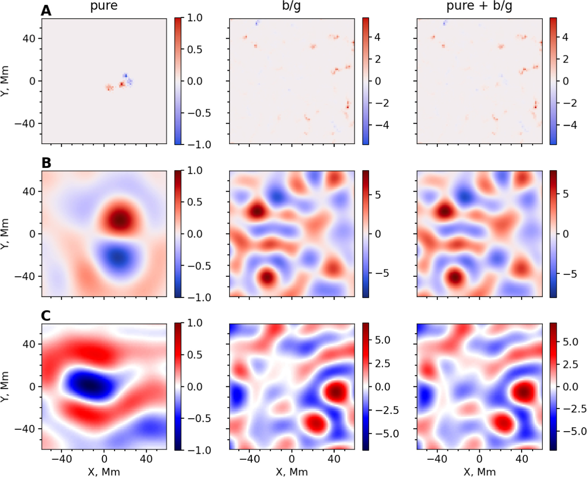
Figure 6. Top row: magnetic field; middle row: vorticity; bottom row: inflows. Left column: pure features generated using the procedure in Section 4; middle column: observed QS (background), with amplitudes greater than pure features, to imitate the S/N of observations; right column: adding the left and middle column images and normalizing to 1.
Download figure:
Standard image High-resolution imageThe i-S/N is a hyperparameter of the machine, in that we control it externally and it influences the prediction accuracy of the machine. Thus, it is natural to anticipate different training accuracies and predictions based on different input i-S/Ns. This is demonstrated for the ensemble-averaged EAR images of bipolar fields, radial vorticity, and horizontal divergence, in the [−24, −18] hr period in Figure 5. We interpret this figure as follows: the machine learns to detect increasing numbers of poor-S/N AR features as it is trained on noisier synthetic AR images (the top panel, showing an increasing number of positive—"true-positive" or "TP"—detections with increasing i-S/N/noisier data), but, at the same time, it becomes more susceptible to false-positive predictions in QS images (suggested by the bottom panel, with the drop in validation accuracy with increasing i-S/N/noisier data).
5. Training and Testing on Synthetics
Although the goal is to understand the predictions of the machine on observed AR images, it is useful to first illustrate the predictions on synthetic ARs and observed QS images.
5.1. Training
Data sets in machine learning are conventionally split into "training," "validation," and "test" data. During training, the machine is only allowed access to the training data and it does not use validation data to adjust the weights and biases of the neural network. Rather, at every epoch, the machine's performance is evaluated on the validation data. Therefore, the criterion that all the samples in the test data set remain unseen by the machine during the training may be satisfied by using the same data set for the "validation" and "test" data. Below are the "training" and "test" data splits and model parameters:
- 1.training: 10,000 images—5000 AR, 5000 QS;
- 2.test: 2000 images—1000 AR, 1000 QS;
- 3.learning rate: 10−5, epochs: 30, batch_size: 30; and
- 4.optimizer: Adam, loss: binary_crossentropy, metric:binary_accuracy.
5.2. Testing
The machine is tested on 1000 synthetic AR and 1000 observed QS images. Table 1 summarizes the results for the test data set, with the i-S/N chosen from the random normal distribution . AR(1) and QS(0) in Figure 7 (and Figure 8; the first two columns of the figure) are where features are correctly detected to be present and absent, respectively. Two other results that the test on synthetic AR and observed QS demonstrates: (1) as seen from the average of all the AR(1) and QS(1) in Figure 7 (and Figure 8), the model has learned to identify the desired magnetic and flow features in the both AR and SQ images; and (2) it also misses detection when the feature is dominated by large background noise, as evidenced by the average of all the AR(0). As explained in Section 4.3 and Figure 5, increasing the i-S/N might increase AR(1) in the observed AR, but will simultaneously increase QS(1) in the QS, reducing overall accuracy. The discussion of accuracy is limited to testing on synthetics merely as an illustration, as our primary aim is to study if the AR-like flow and magnetic field features are unique to ARs alone.


Figure 7. Averages of the images belonging to the four outcomes. The panels in the row are saturated to the color scale of AR(1) (the first panel in the row). The above results are summarized in Table 1. Results corresponding to magnetic bipolar fields and radial vorticity are shown in Figure 8 in Appendix B.
Download figure:
Standard image High-resolution image
Figure 8. Machine-learning results for synthetics: the averages of the images belonging to the four outcomes. Top row: magnetic bipolar fields; bottom row: radial vorticity. The panels in a row are saturated to the color scale of AR(1) (the first panel in the row). The above results are summarized in Table 1.
Download figure:
Standard image High-resolution imageTrue Skill Statistics provides a measure of the accuracy of the machine in feature detection/classification tasks. It is computed using the rates of correct detections of both classes (1 and 0) in the test sample—that is, how many AR and QS are mapped to 1 and 0 as a fraction of their total sample size, respectively. For our case, we use the below formula:

6. Results on Observations and Interpretation
To make predictions on the observations, we use the inflow machine at pre-emergence times (t < 0) and the outflow machine on post-emergence (t > 0) flow images. The model outputs for the ARs in the nine time intervals are noted. The AR flow images in each interval are categorized according to whether they contain or do not show a flow signal (machine outputs 1/0). The results are plotted in Figure 3(A).
Contrary to the impressions gained from average measurements in ensemble studies, only some ARs contain inflow signatures. We find that the category of "AR flows" is broad, i.e., there exists a subclass of ARs that do not show any flow features. In each time interval, the contrast between the middle and bottom rows in Figure 3(A) shows that the model was able to pick out those particular ARs that contain the AR-like inflow (t < 0) and outflow (t > 0) features from the entire set. The fraction of total ARs in a given interval with or without these AR-like flow features is shown above each panel in the middle and bottom rows. Based on this model, anywhere between 40% and 60% of ARs contain features. For instance, in the fourth column (Ti = −15 hr), there are 107 ARs, of which 58% (62 ARs) contain an inflow, whereas it is absent in the other 42% (45 ARs). We trained multiple independent machines, on training samples generated afresh each time, to check for consistency in the predictions, i.e., to test whether the same set of ARs is categorized as 1/0. We find that the predictions remain consistent to within 3%, i.e., for an observational sample size of 100, outputs for only three ARs vacillate around 0.5 in the sigmoid output, while in different models, one or more of these three may switch between 1/0—samples that are close to the decision boundary, since they are harder to classify. This is understood to be machine error, rather than the actual noise statistics of the observed AR flows.
A cursory glance at the middle row of Figure 3(A) reveals that ARs with pre-emergence inflows seemingly evolve into outflows post-emergence. To verify if this is the case, we plot a Venn diagram (Figure 9(A)) for two representative sets—(62) ARs that show inflows at −15 hr and (64) ARs that show outflows at +15 hr. We refer to these two sets as "inflow ARs" and "outflow ARs," respectively. Roughly equal numbers of ARs are present in the three regions of the Venn diagram, i.e., ARs with pre-emergence inflows may or may not show outflows post-emergence.
The overlaid magnetic field contours in the middle and bottom rows of Figure 3(A) indicate an absence of meaningful correlation between flow features and magnetic fields, i.e., the presence of bipoles has little to no bearing on the presence of inflows/outflows in their vicinity.
6.1. Weak Evidence for the Existence of Signature Flows in ARs
In order to ascribe flow features as ARs, a comparison with QS flows allows for the establishing of a baseline—the threshold above which flow features may be correlated to large-scale magnetic fields with appropriate confidence. For this purpose, we collect 110 QS horizontal divergence flow images and evolve them for 54 hr/nine contiguous 6 hr intervals (the same duration over which the flows around ARs are studied). To place error bars, we evolve 30 different batches of 110 samples over the nine intervals to obtain the mean and standard deviations.
Figure 3(B) shows the ensemble average of 110 samples (top row) and the fraction of samples with/without identified AR-like flow features in the middle and bottom rows, respectively. The CNN model does not recognize AR-like flow features as unique only to ARs. There is a non-negligible baseline rate (35%–40%) with which these features also appear in QS flow fields. Since we train our model on synthetic flows, which are averaged over many supergranules in QS, it may be predisposed to finding AR-like flow features in QS. That the CNN model finds these features in both AR and QS images indicates that flows associated with ARs may not be physically distinct from background supergranular flows.
In Figure 9(B), we compare the rate at which AR-like inflows and outflows (the fractions of total samples in which flow features are detected by the CNN model) appear in both AR and QS versus time t before and after emergence. For the sake of completeness, ARs in all nine intervals are passed through both inflow and outflow CNN models to estimate the corresponding occurrence rates over the course of emergence. 30 batches of 110 QS samples are also evolved and tested by the CNN model to obtain mean and 1σ standard deviations of the QS rates (the shaded blue and red curves in the left and right panels). The AR prediction rate is almost constant with time for the QS maps, indicating that the background is statistically time invariant. We apply the same QS error bars to the AR rates, with the assumption that the noise statistics are similar. Consequently, these features are present in only a fraction of AR samples, and the statistical significance of the rate at which they appear above the background (≃3σ only at −15 hr) may be debatable, indicating a lack of robust emergence-related flow signatures (from the current sample size). The results indicate a weak tendency for flux to emerge near supergranular inflows. Surface AR inflow amplitudes of 60 m s−1 are much weaker than supergranular speeds of ∼300 m s−1, pointing toward an imperfect alignment of emergence location and supergranular cell boundaries. While the correlation between AR inflows and emergence location and supergranular boundaries was explored in Birch et al. (2013, 2019), conclusive evidence has been lacking until present.

Figure 9. (A) Venn diagram illustrating the correlation between "inflow ARs" and "outflow ARs." (B) Statistics of AR (solid lines) and QS (shaded region) vs. time, showing the fraction of total samples containing AR-like inflows (left) and AR-like outflows (right). The vertical green dashed line marks the emergence time t = 0.
Download figure:
Standard image High-resolution image6.2. Weak Evidence for Magnetic-buoyancy-assisted Emergence
Next, we carry out tests to explore two phenomena predicted to be associated with magnetic-buoyancy-assisted flux emergence: (1) a hypothesized retrograde flow (Fan 2008; Weber et al. 2011; −vx feature) that appears in numerical simulations and has been explained as arising due to angular momentum conservation; and (2) an enhanced time rate of change for flux (appearing at the surface due to additional upward force), as compared with the purely convectively driven flux scenario. In numerical simulations of buoyancy-boosted flux emergence in near-surface layers (Cheung et al. 2010; Rempel & Cheung 2014), and in observations (Toriumi et al. 2012), outflows of the order of kilometer per second magnitudes (as compared to the inflows of ∼50 m s−1 amplitudes seen in Birch et al. 2019) are seen near the emergence location. Therefore, we check if outflow ARs show retrograde flows and/or elevated flux growth rates at the surface compared to inflow ARs, a possible sign that magnetic buoyancy is a driver.
The average velocity in the x-direction, , is computed as the average over a contour enclosing the inflow region for the 62 inflow ARs and the outflow region for the 64 outflow ARs (Figures 10(A) and (B)), as these are the characteristic flow features of these two sets of ARs. We only include a sufficiently strong boundary around the inflow/outflow; weak portions of the inflow/outflow feature merge into the neighboring convective background features and we therefore choose to avoid including them. This is achieved by trial and error and setting the threshold to be 1.5 × 10⁻⁶ s−1 in the horizontal divergence image.


Figure 10. (A) Contour for for inflow ARs. (B) Contour for for outflow ARs. (C) Contour for flux and flux rate of change. (D) Illustration of near the emergence location (solid lines) in "inflow ARs" (left panel) and "outflow ARs" (right panel) vs. time, along with in QS (shaded region) inside an area of the same contour as chosen for the ARs. (E): Unsigned flux Φ (left panel) and time rate of change of Φ (right panel) for "inflow ARs" and "outflow ARs." The vertical green dashed line marks the emergence time t = 0. The error bar heights in (D) and (E) are ±1σ.


Download figure:
Standard image High-resolution imageWe obtain versus time for both inflow and outflow ARs by evolving them over the nine intervals, and we plot them in Figure 10(D) as solid lines. To ensure that the in the ARs is above the background, we compute QS values of . We gather 30 batches of 62 QS images containing AR-like inflows (output 1 in the inflow machine) and 30 batches of 64 QS images containing AR-like outflows (output 1 in outflow machine) over the nine intervals. Mean and 1σ standard deviations of the baseline are plotted as the shaded regions in the two panels. We again place the same QS error bars on the AR . We measure no statistically significant retrograde flow (negative ) at the surface in either the outflow or inflow ARs. However, we detect a strong prograde flow in the outflow ARs, post-emergence, which might be correlated with the leading polarity of the bipoles moving more quickly away from the polarity inversion line than the following polarity (Schunker et al. 2019).


To check if flux emerges at a more rapid rate in outflow ARs compared to inflow ARs, we choose a contour such that it sufficiently encloses the bipoles in the ensemble-averaged magnetograms of these two sets (Figure 10(C)). We then compute Φ = ∫∣ B ∣ dA within that contour, using the same contour for both the sets, which is in turn obtained from the ±25 G contours associated with the average of 113 magnetograms at +15 hr. Φ is plotted in Figure 10(E), left panel. To place 1σ error bars, we estimate the standard deviation from within the 62 inflow AR magnetograms and the 64 outflow AR magnetograms. Next, to compare the time rate of change of flux, is obtained (right panel), which may tell us if the flux of the outflow ARs rises faster, i.e., if their net unsigned flux at the surface increases faster than that of the inflow ARs before the emergence time. Figure 10(E) shows the time rate of change of flux for the small number of outflow and inflow ARs in our data set. We find that for most time periods, the rate of change is consistent between the inflows and outflows. However, at T = −3 hr, the outflow's rate of change is greater than the inflow by 2σ–3σ. This coincides with the maximal time rate of change for both inflow and outflow ARs. We note that the small number of samples available for both inflows and outflows likely leads to poor estimates of the error bars, and caution must be taken when interpreting the significance of these two data points. Overall, the time rate of change of flux in the emerging inflow and outflow ARs is fairly consistent (compared to the order-of-magnitude difference suggested by previous authors), lending little support to the hypothesis that outflow ARs, enhanced by magnetic buoyancy, emerge considerably more quickly.

7. Discussion: Comparison with Simulations
Helioseismic studies of EARs, which attempt to infer pre-emergent signatures below the surface using acoustic waves, suffer from low S/N beneath the photosphere, leading to a large spread among the findings (see, for instance, the introductory section of Birch et al. 2013). It is not possible to make assertions about the subsurface flow and magnetic field dynamics from this present study, although we may possibly rule out flux emergence models that misalign with our observations. A major difficulty in modeling the flux emergence process over the vertical extent of the convection zone is the stark density contrast between the top and the bottom layers, placing a steep cost on numerical calculations. Simulations are thus carried out sometimes by only modeling the emergence in the top ∼20 Mm (including the photosphere), over which the density drops sharply and the thermodynamics of the plasma is complicated by ionization and radiative effects (Nordlund et al. 2009). A challenge in these setups is the initiation of flux emergence, since these simulations do not capture large-scale dynamo processes that produce the emerging magnetic field in the first place. Common approaches are: passive flux emergence, by imposing a magnetic field in convective inflow regions; active flux emergence, in which a flux structure (typically a semi-torus) is driven into the simulation domain across the bottom boundary; and the insertion of a buoyant flux tube. The details of the resulting flux emergence in terms of speed are dependent on the specifics of the setup. We briefly review results from relevant near-surface simulations to compare with our inferences.
Radiative MHD simulations of uniform, untwisted, weak (1 kG) magnetic fields rising from 20 Mm below the photosphere (Stein et al. 2011; Stein & Nordlund 2012; passive flux emergence) find the rise speed to be of the same order as the simulated convective upflows at these depths. Their study further implies that downflow lanes in intermediate-sized convective cells (presumably supergranular boundaries) mainly serve to dictate the locations where bipolar fields form, commensurate with the findings of simulations of AR formation in global-scale solar convective dynamos (Chen et al. 2017). Our conclusions also moderately align with this scenario. Supergranular boundaries and emergence locations are correlated (although weakly). Moreover, Stein & Nordlund (2012) suggest that the combined actions of up- and downflows on flux tubes in a supergranular-sized region (∼30 Mm) are sufficient for them to form ARs of similar sizes, i.e., magnetoconvection alone is enough to produce ARs.
Active flux emergence setups in which a magnetic half-torus was kinematically driven across the bottom boundary condition were considered by Cheung et al. (2010) and Rempel & Cheung (2014). Birch et al. (2016) showed that the resulting horizontal flows were too strong compared to observations, unless the vertical flows associated with flux emergence were comparable to typical convective upflows (<150 m s−1 at a depth of 20 Mm), also indicative of a more passive flux emergence process.
Recent attempts (Toriumi & Hotta 2019; Hotta & Iijima 2020) to overcome the drawbacks of flux emergence simulations over limited vertical extents have focused on expanding the domain to cover the entire convection zone and to allow the dynamics of the flux tube to naturally play out through the interaction of convective flows and magnetic fields. Unlike previous setups, they started from a buoyant magnetic flux tube inserted into the volume of the simulation domain. They found that the rise speed of the flux tube was ∼250 m s−1 at 18 Mm below the photosphere; this exceeds the upper limit of 150 m s−1 at 20 Mm reached in a study by Birch et al. (2016) of magnetoconvection simulations constrained by observed surface flows around 70 ARs. Recent follow-up work by Kaneko et al. (2022) has shown that flux emergence is strongly influenced by the interaction with convective flows throughout the convection zone. To that end, they repeated their flux emergence setup more than 90 times, exploring a variety of initial locations for the flux tube.
The lack of correlation between AR-like flow features and large-scale magnetic fields, as seen from the present analysis, suggests that flux emergence is dominated neither by supergranular-scale convective flows nor by magnetic buoyancy. Other near-surface simulations (Cheung et al. 2010; Rempel & Cheung 2014; Chen et al. 2017), reasonably in line with the conclusions of previous studies (Stein et al. 2011; Stein & Nordlund 2012), have found that supergranular-scale mean flows tend to oppose the assimilation of magnetic elements into similar polarities. This assimilation is counteracted by a Lorentz force due to the correlation between small-scale fluctuations in velocity and magnetic fields. We thus speculate that flux emergence and the formation of coherent bipoles and monolithic sunspot structures are driven by small-scale turbulent flows (of the order of few granules or a length scale of a few megameters), rather than large-scale mean flows with supergranular length scales (∼30 Mm), as obtained here using LCT. Although here we only analyze near-surface flows, convection in the deeper layers (below 20 Mm), imaged using seismic techniques, is also likely to play a role in setting up the observed AR-scale magnetic fields at the surface.
Acknowledgments
The machine-learning part of the research was carried out with the Intel®Xeon®CPU E5-2620 v3 GPU in the Department of Astronomy and Astrophysics at the Tata Institute of Fundamental Research, Mumbai, India. The parallel processing for the analysis of intensity and magnetogram files was done on the Intel®Xeon®Platinum 8280 CPU.
Funding. This material is based upon work supported by the National Center for Atmospheric Research, which is a major facility sponsored by the National Science Foundation, under Cooperative Agreement No. 1852977. This research was supported in part by a generous donation (from the Murty Trust) aimed at enabling advances in astrophysics through the use of machine learning. The Murty Trust, an initiative of the Murty Foundation, is a not-for-profit organization dedicated to the preservation and celebration of culture, science, and knowledge systems from India. The Murty Trust is headed by Mrs. Sudha Murty and Mr. Rohan Murty. This material is based upon work supported by Tamkeen under the NYU Abu Dhabi Research Institute grants G1502 and CASS.
Author Contributions. S.M.H., P.M., and C.S.H. designed the research. P.M. performed all the analysis. C.S.H. obtained the data. S.D. and P.M. interpreted the machine-learning results. M.R. helped with the conclusion.
Data and Materials Availability. The HMI data are available on the JSOC export site http://jsoc.stanford.edu. The codes for machine learning, generating synthetic flows, and magnetic fields are available from the author upon request.
Software: pyFLCT (Welsch et al. 2004; Fisher & Welsch 2008; The SunPy Community et al. 2020), tensorflow (Abadi et al. 2016), numpy (Harris et al. 2020), scipy (Virtanen et al. 2020), skimage feature detection (Van der Walt et al. 2014), netdrms v9.3, 5 mtrack v2.6. 6
Appendix A: pyFLCT
pyFLCT takes as input a pair of intensity images with time separation (45 s) between adjacent images. The routine is designed to focus on localized regions in the image pairs, by fading out the contribution from areas outside of the subregion, and to obtain velocities for such subimages. This process is repeated until the whole image is covered. The extent of the localization desired is given by the input sigma, which we set to 5 pixels (∼2.5 Mm). We run the routine over a given time interval Ti , where i = 1...9, and obtain the average velocity for that interval. As we are only interested in supergranular-scale features, we smooth [vx , vy ] with a Gaussian of full width 10 Mm and then obtain the horizontal divergence and radial vorticity (see Equations (1) and (2)).
Appendix B: Input Image Size
Our tracked data products of 115 ARs are 32° × 32° in spatial size. The region of interest is only near the center of the image, where the AR is set to emerge; prior studies (Birch et al. 2019; Gottschling et al. 2021) have shown flows associated with EARs to be limited (∼7°) in spatial extent. Therefore, we use images of a smaller size, of 10° × 10°, for training the machine. Moreover, we interpolate the images onto a coarser grid of resolution 1.4 Mm, as small-scale features are not relevant for successful training. Synthetic AR images are generated on this grid and QS images are randomly oversampled from the larger image to reduce computation load. That is, instead of obtaining multiple separate 10° × 10° QS observations, 150 different images of the same area are obtained from a 32° × 32° image in a process called oversampling (see Figure 11).

Figure 11. A representative 32° × 32° QS horizontal divergence flow map. The black squares overlaid on the map indicate random 10° × 10° oversampling. While there is of course a chance of partial overlap between smaller images, machines see them as unique samples. This is also done for the bipolar field and radial vorticity images.
Download figure:
Standard image High-resolution imageAppendix C: Complete Test Results on Synthetics and Observations
The trained model is tested on bipolar field, radial vorticity, and horizontal divergence images, in the nine time intervals T1 to T9, for all the ARs in a given interval. We do not show the QS results here again. The number of available ARs decreases the farther back from the emergence time one observes, as ARs tend to move outside of the desired field of view (±50° central meridian distance). The total number of ARs for the nine Ti s, along with the number of 1 and 0 detections, are tabulated for the bipolar field, radial vorticity, and horizontal divergence images and noted down in Table 2. Figures corresponding to Table 2 are shown in Figure 12. We draw the following conclusions from the results:
- 1.The model shows all 115 ARs as containing bipolar magnetic fields from T6, which is the interval closest to the emergence time and forward (see Figure 12(A), last three columns).
- 2.The number of ARs predicted by the machine as containing bipoles (bipolar fields) and double vortex rolls (radial vorticity) steadily increases with time. But the number of ARs containing inflows/outflows (horizontal divergence) peak at −15 hr and +15 hr, respectively.
- 3.The strengths of the magnetic field and vorticity, in bipolar fields and radial vorticity images, respectively, also steadily increase with time, while the strengths of the inflows in the horizontal divergence images peak around −15 hr.

Figure 12. Machine-learning results for observations. (A) LOS magnetic field (in units of Gauss). (B) Radial vorticity (in units of 1 s–1). (C) Horizontal divergence (in units of (1 s–1)). In each panel, "full," "1," and "0" denote the ensemble averaging of all the ARs, the ARs in which the machine detected a flow/magnetic field feature, and the ARs in which it did not detect a flow/magnetic field feature.
Download figure:
Standard image High-resolution imageTable 2. Results for Observations
| –33 hr | –27 hr | –21 hr | –15 hr | –9 hr | –3 hr | +3 hr | +9 hr | +15 hr | |
|---|---|---|---|---|---|---|---|---|---|
| Total | 88 | 93 | 98 | 107 | 115 | 115 | 115 | 113 | 113 |
| Bipolar fields | 1: 32 | 1: 42 | 1: 54 | 1: 80 | 1: 103 | 1: 115 | 1: 115 | 1: 113 | 1: 113 |
| 0: 56 | 0: 51 | 0: 44 | 0: 27 | 0: 12 | 0: 0 | 0: 0 | 0: 0 | 0: 0 | |
| Radial vorticity | 1: 43 | 1: 45 | 1: 52 | 1: 60 | 1: 68 | 1: 86 | 1: 93 | 1: 94 | 1: 91 |
| 0: 39 | 0: 48 | 0: 46 | 0: 47 | 0: 47 | 0: 29 | 0: 22 | 0: 19 | 0: 22 | |
| Horizontal divergence | 1: 40 | 1: 47 | 1: 56 | 1: 62 | 1: 64 | 1: 57 | 1: 47 | 1: 57 | 1: 64 |
| 0: 48 | 0: 46 | 0: 42 | 0: 45 | 0: 51 | 0: 58 | 0: 68 | 0: 56 | 0: 49 | |
Note. 1/0 denote the number of ARs in which the model detects/fails to detect the flow/magnetic field feature.
Download table as: ASCIITypeset image
Appendix D: Absence of Strong Correlation between Magnetic Fields and Flows
Prior studies have shown a correlation between emerging AR flows and magnetic flux. As is shown in the Venn diagrams (see Figure 13), we do not measure substantial correlations between flows and magnetic fields in the observations of ARs. Rather than imposing a flow–magnetic field correlation a priori, it is more objective to discover if any such connection exists through independent machines for these features.

Figure 13. Venn diagrams depicting correlations between flow and magnetic field features in observations. Below each Venn circle in a panel, the feature and the machine prediction are indicated—for instance, 1D (−15 hr) means the ARs that the machine predicted as containing inflows in the interval −15 hr. The number of these ARs is given inside the Venn circle.
Download figure:
Standard image High-resolution image