


Abstract
The one consistent technique for remotely estimating the magnetic field in plasma has been Faraday rotation. It is only sensitive to the portion of the vector parallel to the propagation path. We show how to remotely detect the portion of the vector that is perpendicular using a modified measurement. Isolating this electromagnetic propagation wave mode to measure the magnetic field enables us to (i) study more about the magnetic field vector in plasma, (ii) reduce error in total electron content measurements, and (iii) discover new magnetic field information from archived data sets. The Appleton–Hartree equation is used to verify a new approach to calculating the phase change to an electromagnetic wave propagating through a plasma at frequencies larger than the gyrofrequency, the cyclotron frequency, and the upper hybrid frequency. Focusing on the perpendicular propagation modes, the simplified equation for the integrated path effect from a perpendicular magnetic field is calculated. The direction of the perpendicular component is unknown, because the magnetic field is squared. Isolating the magnetic term in the equation with dual frequency waves is shown. We also show how to eliminate the magnetic field contribution to total electron content measurements with a similar approach. In combination with Faraday rotation, the degeneracy of the magnetic field vector direction is reduced to a cone configuration.
Export citation and abstract BibTeX RIS

Original content from this work may be used under the terms of the Creative Commons Attribution 4.0 licence. Any further distribution of this work must maintain attribution to the author(s) and the title of the work, journal citation and DOI.
1. Introduction
One facet of space weather consists of plasma conditions of the Sun, solar corona, solar wind, Earth's local magnetosphere, and the ionosphere, as well as other regions of interplanetary and intraplanetary space. Studying, modeling, and predicting this aspect of space weather requires understanding the magnetic field (e.g., Viall & Borovsky 2020). Radio frequencies are best to remotely measure magnetic fields for the vast majority of space (e.g., Kooi et al. 2022).
The propagation of radio waves through plasma depends on the electromagnetic (EM) wave frequency relative to the plasma's cyclotron, plasma, and hybrid frequencies. In the high-frequency regime, where the EM wave frequency exceeds the plasma, cyclotron, and upper hybrid frequencies, the EM wave assumes four different plasma wave mode configurations: (1) the ordinary "O-mode," (2) the extraordinary "X-mode," (3) the left-handed circularly polarized "LCP-mode," and (4) the right-handed circularly polarized "RCP-mode." Note that O-/LCP-modes and X-/RCP-modes are the same wave modes but occurring at different orientations relative to the path. As with many fields of science, these terms are not uniformly used to describe the same conditions. Table 1 lists the definitions that we will be using in this paper. Ionospheric radio experts will use "O-mode" and "X-mode" for what we have defined as "LCP-mode" and "RCP-mode." To reduce confusion, we will be referring to the O-mode as the "non-B-mode" and X-mode as the "B⊥-mode" to distinguish between these definitions when possible. For example, the following statement in Poole (1985), "Thus the direction of the electric vector measured in the horizontal plane of the antennas moves clockwise with time, looking down on the antennas. This corresponds to the extraordinary mode," contains two issues; the first is that magnetic field is not present in the description of the mode, and the second is that it describes one of the circular polarization modes of the observing antenna. Another example is Walden (2016): "When the thumb points in the direction of the magnetic field B0, the rotation of the extraordinary-wavevectors is given by the fingers of the right hand; the rotation of the ordinary-wavevectors is given by the fingers of the left hand." With respect to the equations in Table 1, this description meets our definition of the RCP- and LCP-modes specifically.
Table 1. Radio EM Propagation Dispersion Relations and Description of X-mode (B⊥-mode) Vector Orientations
| O-mode (non-B) |

|
| X-mode (B⊥) |
|
| RCP-/LCP-mode (B∣∣) |
|
| *Note |
 , , |
| X-mode vector orientations | B0 and B⊥ are in the z-direction |
| E1y and U1y are in the y-direction | |
| k, E1x , and U1x are in the x-direction | |
Notes.
ω is the frequency of the transmitted radio signal, ωpe
is the plasma frequency, Ωce
is the cyclotron frequency, n is the index of refraction, e is the electron charge, B0 is the background magnetic field, me
is the electron mass, N is the electron density, and  0 is the permittivity of free space. In the X-mode (B⊥-mode) description, k is the wavevector, U1 is the perturbed electron density, E1 the electric field, and B1 the magnetic field. "*Note" provides the MKS version for plasma and cyclotron frequencies used in the table. Adapted from Kivelson and Russell (1995).
Download table as: ASCIITypeset image
The non-B-mode propagates regardless of whether a magnetic field is present in the plasma. It is the fundamental propagation mode for the interaction of an EM wave with charged plasma particles. The remaining modes exist when a magnetic field is present in the plasma. As the EM wave propagates parallel to the magnetic field, the gyromotion of the electrons around the magnetic field, right-handed cyclotron motion, comprises a circularly birefringent medium. The EM wave assumes not just non-B-mode propagation, but also RCP- and LCP-mode propagation. These circularly polarized modes are the cause of the well-known phenomenon of Faraday rotation, which enables us to measure one component of the magnetic field vector in the plasma. Whichever of the RCP-/LCP-modes is in the handedness of the electrons gyromotion has a greater phase velocity than the other; this is a function of whether the magnetic field is parallel or antiparallel to the EM wave. If the magnetic field is parallel to the EM wave propagation direction, then the RCP-mode has the greater phase velocity and vice versa. What is not obtained with Faraday rotation is a measure of the full strength of the magnetic field vector. That information is obtained in combination with the B⊥-mode.
2. Perpendicular B-mode
The fourth mode, the B⊥-mode, occurs when the magnetic field is perpendicular to the EM wave propagation direction. The O-, RCP-, and LCP-modes are used for many different applications of plasma remote sensing (examples in solar physics include Bird & Edenhofer 1990; Bertotti & Giampieri 1998; Miyamoto et al. 2014; Efimov et al. 2018; Jensen et al. 2018; Kooi et al. 2022; and the references therein). Until now, the B⊥-mode has not been studied.
To investigate the B⊥-mode, we analytically calculated how the B⊥-mode would modify the phase of the EM wave as it propagates. Then we modeled EM wave propagation through a plasma having a perpendicular magnetic field using the fundamental plasma Appleton–Hartree equation. Finally, we compared these two solutions and discovered how the B⊥-mode manifests.
The analytic calculation of the B⊥-mode begins with a general equation for how the phase angle changes,

where φ is the phase angle, S is the propagation path, vφ is the phase velocity, vgroup is the group velocity, and ω is the angular frequency of the wave. The 1/2 on the right side of the equation results from what we assume is averaging the difference in phases between the phase and group velocities. At issue is that there is a factor of 1/2 on the right side of the equation that must be accounted for in the known non-B-mode and RCP-/LCP-modes products shown in Equations (4) and (6). This is a topic of future study with finite-difference time-domain modeling.
In the case of EM waves, the phase and group velocities are a function of the index of refraction, n, and the speed of light, c. As a result, Equation (1) becomes the following. Note that the group velocity differences between the B⊥-mode and non-B-mode are insignificant in the calculation, being of the order ω−4. An issue with the circularly polarized modes will arise in oblique propagation, but that will be discussed in future work.

The indices of refraction in Table 1, when substituted for n in this equation, become the following after expanding and dropping the insignificant terms.
O-mode (non-B-mode):

Under the condition of radio frequency signal propagation described in Jensen et al. (2016), this equation becomes the form of which is important in isolating this effect, where φS is the received phase, the completed integral from source to receiver, and d φS /dt = Δω.

RCP- and LCP-modes (B∥-modes):

which yields the Faraday rotation equation

Finally, the X-mode (B⊥-mode)

where q = ∣ − e∣ in this formulation, e is the electron charge, me
is the electron mass, εo
is the permittivity of free space, N is the electron density, and B is the magnetic field strength along the path S (∥) in the case of RCP- and LCP-modes or perpendicular to the path (⊥) in the case of the X⊥-mode. The frequency is  .
.
Notice that the non-B-mode is present in Equations (5) and (7) as the first term. The Appleton–Hartree equation comprises the full solutions to each of these propagation modes. Unfortunately, it is difficult to work with; hence, this approach shown in Equation (7) provides a solution that is easier to work with.
3. Testing
Using the Zenodo-published code for Appleton–Hartree (Jensen et al. 2024), we initially calculated the accuracy of Equations (3) and (7) in this paper. Figure 1 shows that our calculations are excellent approximations for Appleton–Hartree. However, a comparison of Δφ quickly shows the effect of the Taylor expansions used in the calculations. Figure 1 (bottom row) shows the error in the difference in Δφ grows even after a few meters; over 1 × 10¹⁰ m, this is significant.
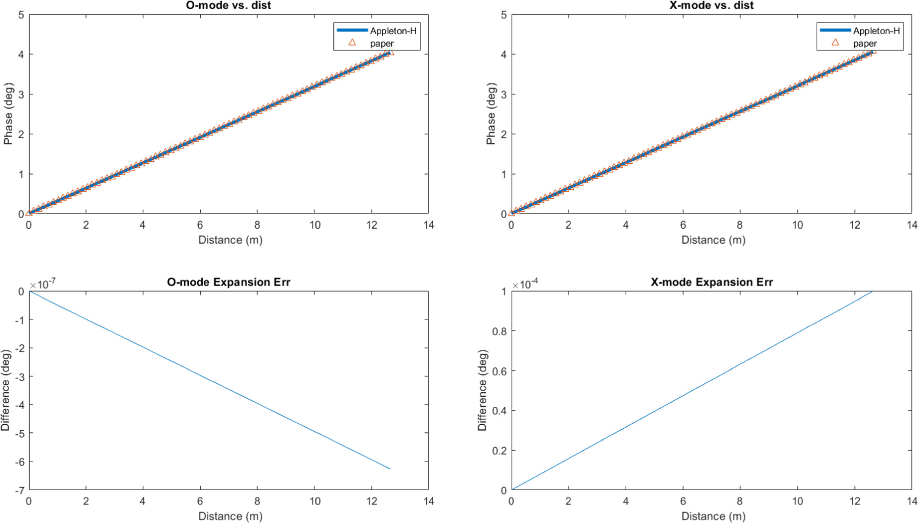
Figure 1. Top panels: Appleton–Hartree simulation (blue lines) of high-frequency EM wave propagation in a plasma without a magnetic field (non-B-mode only) is shown to the left and conditions with a perpendicular magnetic field (B⊥-mode) is shown to the right. The calculation for the expected cumulative phase change from Equations (3) and (7) is shown in red. Bottom panels: the accumulating difference between the solutions is shown; this is due to the Taylor expansion used to simplify the Appleton–Hartree solutions. For this figure only, the frequency of the signal was 477 MHz, the plasma frequency was 100 MHz, and the cyclotron frequency was 200 MHz.
Download figure:
Standard image High-resolution imageCurrent technology is not going to provide information on the absolute phase φ change when it reaches the receiver, but it can provide information on how the received phase at the receiver φS
changes with time. This is given by frequency fluctuations  . Changes to φS
(φ observed by the receiver) with time are consistent. This is what is demonstrated in the second and fourth rows of Figure 2. To be clear, Figure 1 (first row) shows the changes in φ along the line of sight S, whereas Figure 2 shows the final received φS
varying with time, which is observed as a non-Doppler frequency shift.
. Changes to φS
(φ observed by the receiver) with time are consistent. This is what is demonstrated in the second and fourth rows of Figure 2. To be clear, Figure 1 (first row) shows the changes in φ along the line of sight S, whereas Figure 2 shows the final received φS
varying with time, which is observed as a non-Doppler frequency shift.

Figure 2. Testing how d/dt varies between electron density (plasma frequency) and magnetic field (cyclotron frequency); the signal frequency is 10 MHz. The top three plots show the case where plasma frequency decreases/increases; the bottom (second row) shows the ± change in d/dt frequency that is utilized in studying TEC. The bottom three plots show the case where cyclotron frequency decreases/increases; the plot in the last row shows the discontinuity in the change. Due to the plasma frequency's greater impact on d/dt, the discontinuity does not change the overall sign of the response. Also visible in this plot's resolution is the floating point error in the Appleton–Hartree calculations with these plasma parameters. The plots used the following conditions: N = 200 cc, B⊥ = 500 nT, S = 1 × 10¹⁰ m.
Download figure:
Standard image High-resolution imageFigure 2 shows two tests run to investigate the impact of different forms of variability. On the first row, the electron density varied by decreasing then increasing in time while the perpendicular magnetic field was consistently decreasing. This produced the expected positive/negative fluctuation well known for studying changes in total electron content (TEC) as seen in the second row plot. On the third row, the electron density was steadily decreasing in time while the perpendicular magnetic field was decreasing then increasing in time. Its effect on the observed frequency fluctuations was significantly less as shown in the plot on the fourth row. However, the discontinuity when the perpendicular magnetic field reverses from decreasing to increasing remains. Note that for the third and fourth rows in this figure, the floating point error in the Appleton–Hartree calculations becomes visible. These were present in the second row; however, the range was too large for the instability to be seen.
We then calculated the propagation of a signal using solar coronal mass ejection (CME) sheath values and distances (B⊥ 500 nT, N 200 cc, S 1 × 10¹⁰ m; see Figure 3) at frequencies too high for the evanescent upper hybrid resonance to absorb (10 and 20 MHz). The 10/20 MHz frequencies were selected as being reasonably low to be sensitive to the B⊥-mode plasma conditions. Undoubtedly, higher frequencies are also sensitive; that is an analysis we will pursue by calculating the oblique magnetic field case.
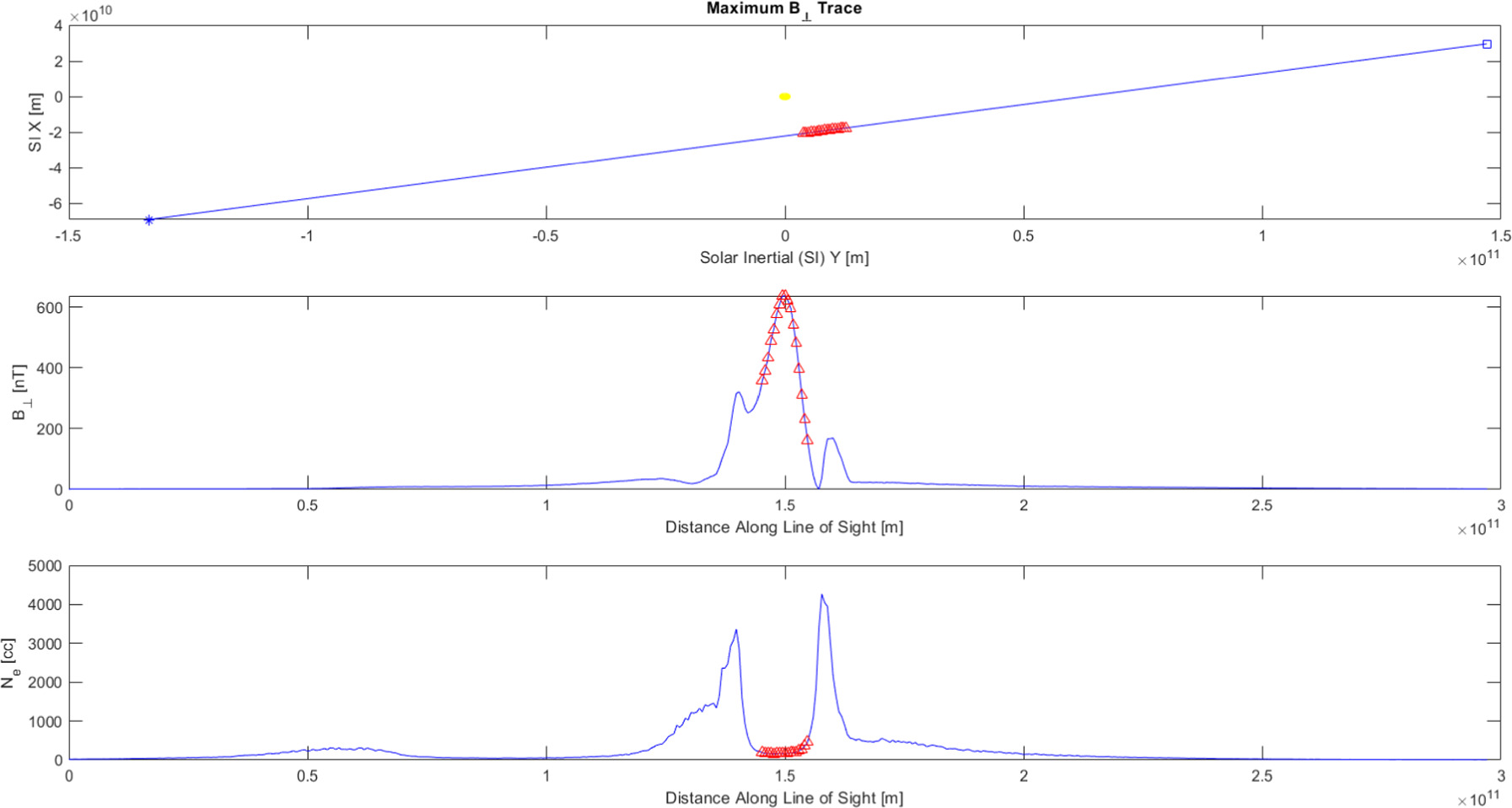
Figure 3. CME values obtained from the Manchester et al. (2014) 2005 May 13 CME MHD simulation. Using the line of sight shown in the top panel (source is the *, receiver is the □, Sun is the yellow circle at the origin), the B⊥ and N parameters at 22:04 UT along the line of sight are shown in the middle and bottom panels. The red triangles show the extent of 1 × 10¹⁰ m over which the values were averaged.
Download figure:
Standard image High-resolution imageThe challenge is to separate the TEC effect from the B⊥-mode. Consequently, we have calculated a method to isolate each, the non-B-mode and the B⊥-mode. To perform this operation, two frequencies must be simultaneously observed. As shown in Equations (8) and (9), subtraction of the frequency fluctuations with a scaled factor enables us to isolate the modes.


where the two frequencies are ω1 and ω2, and the fluctuations observed in their values from plasma alone (eliminating other effects such as Doppler) are Δω1 and Δω2.
A quick back-of-the-envelope calculation can be made to examine the use of Equations (8) and (9) for separating the modes. For this investigation, the CME parameters were used for the whole space uniformly. As can be seen in Figure 3, a uniform distribution of plasma parameters is not realistic, but it is a common first-order assumption when analyzing data. The purpose here is to examine the equations for reproducing the input values. Under the conditions of uniform distribution of density and magnetic field, we can inspect the result of these equations with the following calculations. Note: the less uniform the distribution in density and magnetic field along the line of sight is, the greater the error in using Equations (10) and (11).

and

Figure 4 shows that Equations (3) and (7) performed as expected (ω1 = 10 MHz and ω2 = 20 MHz). Two cases were run; the second is shown in the figure. The first case used the output from Equation (7); it was a perfect fit, which would be the case when using the same equation in Equations (8) and (9). The second case used the phase calculated from the Appleton–Hartree equation, even though it had the floating point problem, as can be seen in the calculation's work. A non-B-mode signal was obtained with Equation (8), and the magnetic field component to the B⊥-mode was isolated with Equation (9), enabling further analysis. A word of caution: the electron density and magnetic field must be evenly distributed along the line of sight (S) for the plots shown in the bottom of Figure 4 to be that accurate. This is a well-known challenge in remote sensing problems, as is how to measure initial conditions. In this case, we need to use other data sets or modeling to obtain TEC(t = 0) and  .
.

Figure 4. Taking the solar wind conditions shown in Figure 3, the ability of Equations (8) and (9) to isolate the parameters is studied using the Appleton–Hartree modeled phases. The primary signal is 10 MHz and the secondary is 20 MHz. The top left plot shows the Equation (8) calculated TEC + TEC(t = 0); the top right plot shows the Equation (9) calculation + its initial value. Using the back-of-the-envelope calculations for 〈N 〉 and 〈B⊥〉, these are compared in the bottom two plots to the initial conditions calculated from the plasma and cyclotron frequencies (input).
Download figure:
Standard image High-resolution image
4. Broader Impact
The formulation in Equations (3) and (7) has implications for other observations. As shown earlier in the discussion on Equation (3), the frequency fluctuations calculated for narrowband artificial signals is assumed to be entirely non-B-mode. This assumption is utilized for a critical infrastructure component: TEC measurements of the ionosphere using Global Positioning Satellites (GPS; e.g., Schreiner & Born 1993; Minter et al. 2007; Dyrud et al. 2008). Equations (7) and (5) show that the B⊥-mode and the B∥-modes similarly impact frequency fluctuations. In fact, since the non-B-mode is linearly polarized, it may be that all TEC observations are actually the elliptically polarized, combined by-product of B⊥-mode and B∥-modes. The B∥-modes can be incorporated into models for data analysis as they are well understood. However, this means that with respect to the B⊥-mode, it is a consistent source of error in ionospheric TEC measurements. Regions where it would have the greatest impact are where the perpendicular magnetic field is stronger relative to the EM wave propagation path, e.g., the auroral oval and paths closer to the horizon. The challenge this paper will address is to discuss an approach to separate the TEC effect from the B⊥-mode.
As we show above, the analysis can be conducted to study the component of the magnetic field perpendicular to the path of the EM wave. The effect of the B⊥-mode on dual frequency, narrowband observations enables reanalysis of older data sets. For example, Cassini 2 and 8 GHz radio sounding observations were collected through Saturn's ionosphere (Tamburo et al. 2023). It is important to note that the direction of this component is unknown. Thus, when combined with the magnetic field analysis from Faraday rotation observations, a cone of vector orientations can be observed. The Faraday rotation gives the magnitude and direction parallel to the propagation path, whereas the B⊥-mode gives the magnitude perpendicular to the propagation path. Extensive analysis to address integration effects is necessary to reach this result; however, this is the first time a full magnetic field magnitude estimation can be made.
5. Summary
The remote observing of magnetic fields is essential to understanding space weather. Thus far, radio frequency observations of plasmas have not taken advantage of the propagation mode containing the perpendicular magnetic field. Instead, it is typically treated as noise. Here, however, the B⊥-mode from the Appleton–Hartree equation is compared to our derivation enabling easier manipulation for studying this phenomenon. After demonstrating that our equation is successful for time-varying observations, we then presented how to isolate the nonmagnetic mode from the B⊥-mode using dual frequency observing.
The equations derived for analyzing the B⊥-mode and non-B-mode separately can be applied to evaluate previously collected and archived data (e.g., Tamburo et al. 2023 for Saturn's ionosphere). It enables the removal of a source of error in GPS TEC measurements through the ionosphere. It also can be incorporated into future spacecraft radio designs for obtaining the full magnetic field magnitude in remote sensing observations (e.g., Jensen et al. 2023). The various applications opened with these equations impact our infrastructure and understanding of the Sun, solar wind, stellar wind, and geospace.
In future work, we will simulate these propagation modes using a finite-difference time-domain model of EM propagation through more complex magnetized plasma to examine the dual frequency observing equations and their performance under a variety of realistic plasma conditions ranging from the ionosphere to the solar corona.
Acknowledgments
ACS Engineering & Safety LLC funded this work. We would like to thank Dr. David Wexler, the Planetary Science Institute, and the University of Utah.