


Abstract
Space plasmas are turbulent and maintain different types of critical points or flow nulls. Electron vortex, as one type of flow null structure, is crucial in the energy cascade in turbulent plasmas. However, due to the limited time resolution of the spacecraft observations, one can never analyze the three-dimensional properties of the electron vortex. In the present study, with the advancement of the FOTE-V method and the unprecedented high-resolution measurements from four Magnetospheric Multiscale spacecraft, we successfully identify the electron vortex and then reconstruct its three-dimensional topology of the surrounding electron flow field. The results of the reconstruction show that the configuration of the electron vortex is elliptical. Comparison between the observation and reconstruction scales of the vortex indicates the reliable reconstruction of the flow velocity. Our study sheds light on the understanding of the topology and property of the electron vortex and its relationship with kinetic-scale magnetic holes.

Original content from this work may be used under the terms of the Creative Commons Attribution 4.0 licence. Any further distribution of this work must maintain attribution to the author(s) and the title of the work, journal citation and DOI.
1. Introduction
Space plasmas, consisting of electrons and ions, are quite turbulent and can further form different types of flow structures with complex topologies. The flow nulls, also referred to as critical points, are the points where the flow velocities are equal to zero and usually present some characteristics that are different from the surrounding environment (Perry & Chong 1987; Chong et al. 1990). The topological classification for three-dimensional flow fields (for both compressible and incompressible flow) indicates that there are mainly two types of flow nulls in space: the vortex center with the elliptic streamline structures, and the stagnation point with the hyperbolic structures (Chong et al. 1990; Jeong & Hussain 1995; Wang et al. 2020b; Zhang et al. 2023). For example, the Kelvin–Helmholtz vortex (Hasegawa et al. 2004; Otto & Fairfield 2000) or the electron vortex combined with the magnetic hole (MH; Huang et al. 2017b, 2017a) contains the vortex center. Meanwhile, the flow-reversal point in the extensively studied magnetic reconnection region (Sonnerup & Priest 1975; Burch & Phan 2016; Chen et al. 2016) or the dusk-side plasmapause bulge (Fu et al. 2010a, 2010b) presents the features of stagnation points. These two types of flow nulls can be further subcategorized according to a large scale or a small scale of the structures (Wang et al. 2020b), or according to stable or unstable flow nulls (Dallas & Alexakis 2013). These null structures play critical roles in energy transport, conversion, and particle acceleration and are consequently valuable to investigate (Haynes et al. 2015; Burch & Phan 2016; Wang et al. 2022).
As one kind of these flow structures, the small-scale electron vortex is thought to be closely connected with the kinetic-scale magnetic holes (KSMHs; Huang et al. 2017b), and therefore, it is also called the electron vortex MH (Haynes et al. 2015). Moreover, electron vortices are also detected in the current sheets, flux ropes, and magnetic peaks (Wang et al. 2023). Several studies have suggested that the electron vortices play an essential role in the energy cascade in turbulent plasmas (Haynes et al. 2015), weakening the magnetic field and sustaining the magnetic structure (e.g., Huang et al. 2017a, 2017b; Yao et al. 2017; Huang et al. 2018, 2019; Jiang et al. 2020; Wang et al. 2023). For the purpose of figuring out the role of the electron vortex in the dynamic processes in space plasmas, it is necessary to investigate its topology.
Simulation results have demonstrated that the flow nulls are three dimensional in space (Olshevsky et al. 2015; Roytershteyn et al. 2015; Olshevsky et al. 2016). However, until now, due to the unrepeatable satellite observations at limited space points, only a few studies have focused on the topology of the flow nulls with in situ observations.
Reconstruction methods based on plasma measurements and theoretical supports might be a good solution for studying the flow-field structures around electron vortices. Recently, Wang et al. (2020b) proposed a reconstruction method named FOTE-V (first-order Taylor expansion velocity) to reconstruct the flow pattern. FOTE-V is extended and promoted based on the FOTE method (Fu et al. 2015; which is used to reconstruct the magnetic field topology of quasilinear structures with multispacecraft missions) to study the plasma flow fields. Based on four-point data measurements, the FOTE-V method can be used to reveal the 3D properties of the flow nulls with multispacecraft measurements and reconstruct the flow pattern (Wang et al. 2020b).
In this study, we use the FOTE-V method and the multi-point measurements from the Magnetospheric Multiscale (MMS) mission to investigate the electron vortex. We identify the electron vortex successfully, then reconstruct the 3D topology of electron flow, and further estimate its scale. The results show that the FOTE-V method performs well in reconstructing the electron-scale vortex. This paper is organized as follows: the data and method are described in Section 2; Section 3 provides an overview of the events, the detection of an electron vortex, and the reconstructed topology, and finally, we discuss and summarize the results in Section 4.
2. Data and Method
The MMS spacecraft was launched in 2015 and consisted of four identical spacecraft (Burch et al. 2015). The spacecraft separations are variable from 10–160 km, depending on the phase of the mission. Data from the Flux Gate Magnetometer instrument, which provides 128 Hz burst-mode magnetic field data (Russell et al. 2016; Torbert et al. 2016), and the Fast Plasma Investigator instrument, which provides 33.3 Hz electron measurements (Pollock et al. 2016) are used in the present study. The Geocentric Solar Magnetospheric (GSM) coordinate system is adopted in this work unless otherwise specified.
We use the FOTE-V method (Wang et al. 2020b) to identify the flow nulls (critical points) and investigate their topology structures and properties. The FOTE-V method is basically established based on the first-order Taylor expansion of the velocity field around a null point:

where r represents the spacecraft location in space, V is the velocity field at location r , r n is the location of the null point, and ∇ V is the gradient of the velocity field at the null point, which is calculated by the four spacecraft measurements. The FOTE-V method is based on the assumption that the velocity field changes linearly in space, which has been clarified by Wang et al. (2020b). Therefore, the results of the detection of the null points should be treated cautiously and diagnosed carefully. In order to get a reliable result, Wang et al. (2020b) introduced the criteria that the error parameter α should be smaller than 0.4 (α = , to quantify the quality of the FOTE-V results, which is based on the continuity equation in a steady-state plasma ). In our study, apart from this parameter, we further consider another three restrictions to make sure the results are more reliable: (2) The null-satellite distance should be less than 1 di , (di = c/ωpi is the ion inertial scale, and ωpi is the ion plasma frequency); (3) Assuming the gradient of the plasma number density ∇n can be ignored, the continuity equation can be simplified as ∇ · V = 0. Thus, we defined a dimensionless parameter β = , (λ1, λ2, and λ3 are three eigenvalues of the Jacobian Matrix δ V, respectively, is the maximum of the norm of the three eigenvalues), to estimate the accuracy of the results. Following Fu et al. (2015), β is required to be smaller than 0.4; (4) The detected null types should be steady during the observations. We consider the results reliable only when all these criteria are satisfied.


The position data are linearly interpolated to match the cadence of the electron velocity. Then the interpolation-obtained R and Ve are used to calculate the vorticity of the velocity ∇ × V e and to do further identification.
3. Observations and Topological Reconstructions
In this section, we utilize the FOTE-V method to identify the flow nulls within the electron-scale MHs. We chose two representative MH events accompanied by electron vortices in the solar wind and magnetosheath, respectively. We present the flow null identification based on the spacecraft measurement. We also reconstruct the velocity field topology around the null point and try to give a direct and clear scenario of the electron vortex.
The first event here we analyzed was observed by MMS on 2017 December 16, around 18:13 UT, when it was located in the solar wind at (21.6, 10.8, 7.0) RE
in GSM coordinates, which was reported by Wang et al. (2020a). Figures 1(a)–(j) show the four MMS spacecraft measurements of the event observed between 18:13:12.3 and 18:13:13.3 UT, with measurements of MMS1∼4 in black, red, green, and blue lines, respectively. According to the ion omni differential energy fluxes without backflow ion component in Figure 1(a) (here we take MMS1 for example), together with the high ion velocity in Figure 1(j) and the ion density (not shown here but similar to the electron density), we can infer that MMS was in the solar wind, combining with the spacecraft location. In Figure 1(c), there is a distinct magnetic field depression in the total magnetic field Bt
, observed by all four spacecraft in the order of MMS2, MMS3, MMS1, and MMS4, within the region marked by the two vertical dashed red lines. Such a magnetic field depression is identified as an MH, with a duration Dt
of 0.28 s (from 18:13:12.72–18:13:13.00 UT, for MMS1 and 4) and a depression D of 0.85 (from the average magnitude 5.3 nT to the minimum 4.5 nT), with the magnetic vector shear angle of ∼1 5 between two boundaries of this MH. The magnetic depression is accompanied by the increase in electron number density Ne
(Figure 1(d)) and electron temperature Te
(Figure 1(e)), with no apparent change in ion parameters (not shown here). Assuming that the magnetic structure is moving with the plasmas flow, the scale LMH is ∼87.0 km (LMH = Dt
× Vibt
, Vibt
= 311 km s−1, calculated over the 1 s overview interval). Normalized the MH scale by the local ion gyro-radius ρi
(∼149 km) and electron gyro-radius ρe
(∼2 km), respectively, the MH scale is estimated to be ∼0.58 ρi
and ∼42.1 ρe
, indicating that the MH is a sub-proton scale (i.e., kinetic-scale) MH.
5 between two boundaries of this MH. The magnetic depression is accompanied by the increase in electron number density Ne
(Figure 1(d)) and electron temperature Te
(Figure 1(e)), with no apparent change in ion parameters (not shown here). Assuming that the magnetic structure is moving with the plasmas flow, the scale LMH is ∼87.0 km (LMH = Dt
× Vibt
, Vibt
= 311 km s−1, calculated over the 1 s overview interval). Normalized the MH scale by the local ion gyro-radius ρi
(∼149 km) and electron gyro-radius ρe
(∼2 km), respectively, the MH scale is estimated to be ∼0.58 ρi
and ∼42.1 ρe
, indicating that the MH is a sub-proton scale (i.e., kinetic-scale) MH.

Figure 1. MMS measurements of the event on 2017 December 16, (Case 1) and the identification results of velocity nulls using the FOTE-V method. Data are all presented in GSM coordinates. (a) The electron omnidirectional differential energy fluxes of MMS1; (b) the ion omnidirectional differential energy fluxes of MMS1; (c) the total magnetic field Bt ; (d) electron number density Ne ; (e) electron temperature Te ; (f)–(i) three components and the total magnitude of the electron velocities observed by the four spacecraft (the dashed horizontal line represents Vex,y,z = 0); (j) the ion velocities; (k) current density calculated by the curlometer method J ∇×B (solid lines) and by the plasma parameters J p (dashed lines); (l) the vorticity of the electron velocity ∇ × V e; (m) the results of the identification resolved by the FOTE-V method with the four lines presenting the distances between the velocity nulls and each of the four spacecraft (Rns) and the markers demonstrating the velocity null types; (n-o) the dimensionless parameters to quantify the uncertainty of the FOTE-V method, α = , β = (p) the dimensionality factor to predict the dimension of the structures. For (c)–(j) and (m), MMS1 ∼ MMS4 are marked by the black, red, green, and blue lines, respectively, while for (k)–(l), the x/y/z components and total value are marked by red, green, blue, and black lines, respectively.


Download figure:
Standard image High-resolution imageThree components and total magnitude of electron velocity Vex, Vey, Vez, and Vet are shown in Figures 1(f)–(i), respectively. Notice that the velocities here have been eliminated from the background flow velocity for the application of the FOTE-V method. The critical points in the turbulent solar wind are thought to be comoving with the background flow. Thus, we subtract the background flow velocity to resolve the null flow type accurately. The background flow velocity is calculated by the average of the electron flow measured by the four MMS spacecraft ( V eb = ). For this case, the background velocity V eb is ∼[−308, 22.8, −2.0] km s−1 calculated over the overview 1 s interval, and is nearly the same as the background ion flow velocity (Figure 1(j)). The Z-component Vez from the four spacecraft all display an apparent bipolar variation, indicating the spacecraft might cross an electron vortex. Moreover, according to Figure 1(k), the current densities (J∇×B, the solid lines) calculated through the curlometer technique (Dunlop et al. 2002) also show a bipolar variation, which matches the current estimated by the plasma parameters (Jp , the dashed lines) well. Here the plasma current Jp is the average result of the four spacecraft. Since the plasma parameters and the magnetic field are measured by different instruments, these two similar results confirm each other that the measurements are reliable. The bipolar variations appear both in Ve and Jp , demonstrating that the current is mainly carried by the electrons.

The vorticity of the electron velocity is calculated and shown in Figure 1(l). The vorticity during the possible vortex is higher than the ambient, with the max value reaching up to ∼6.6 s−1. Both the bipolar variation of the electron velocity and the vorticity reveal the possibility of the existence of the electron vortex.
In order to verify the existence of electron vortex, we try to identify the null types utilizing the FOTE-V method (Wang et al. 2020b). Figure 1(m) shows the results of the identification of the velocity null types, with the four lines representing the distance from the detected nulls to each spacecraft Rns (MMS1 ∼ 4 in black, red, green, and blue, respectively), and the marker fallen at the minimum distance of each point demonstrating the null type of the electron velocity. The hollow triangle and the cross represent radial nulls (A, B), while the solid triangle and the circle represent spiral nulls (As, Bs), respectively. Meanwhile, the color represents the orientation of the velocity, red for the flow-in field (A, As) and blue for the flow-out field (B, Bs). According to the criteria put forward in Section 2, the null-satellite distance Rns should be less than 1 di (∼72 km). In Figure 1(m), the minimum Rns are mainly within the limitation during the MH interval. It is shown that the majority of the nulls are of the spiral types, which is consistent with the observations of the electron vortex.
Figures 1(n) and (o) show two dimensionless parameters (α = and β = , respectively) to examine the accuracy of the identification of the null properties. Previous studies set 0.4 as the threshold of reliability (e.g., Fu et al. 2015 and Wang et al. 2020b), as shown in Figures 1(n) and (o) by the black horizontal dashed lines. As can be seen from these two panels, the values of α and β at most data points exceed a little above the dashed line during the interval of the vortex. Therefore, we should take much more caution in the subsequent process when choosing the null point to do the reconstruction. Figure 1(p) gives the parameter to predict the dimensionality of the structure, with f2Dv < 0.2 indicating a 2D structure and f2Dv > 0.5 indicating a 3D structure (Wang et al. 2020c). One can see that the time interval with α and β smaller than 0.4 corresponds to f2Dv > 0.5, indicating that the electron vortex here is more likely to be a three-dimensional structure.


After the identification of the null type and other features, we prefer to assume that there exists an electron vortex in the solar wind. Furthermore, we use the FOTE-V method to examine whether there is indeed a vortex center and reconstruct the topology. Considering the restrictions for the reliability of the null type, we choose the null point at 18:13:12.705 UT to undertake the reconstruction of the topology (the vertical dashed blue line in Figure 1). The values of α and β are 11.51% and 23.17%, respectively, and both satisfy the constraints of 40%.
In order to reconstruct the topology intuitively, we establish an eigenvector coordinate system [e1, e2, e3], which is obtained from the Jacobian matrix δ V . At 18:13:12.705 UT, the corresponding eigenvectors of δ V are as follows: n1 = [0.1309+0.4962i, 0.7331, 0.2896-0.3396i], n2 = [0.1309-0.4962i, 0.7331, 0.2896+0.3396i], and n3 = [0.4058, −0.6249, 0.6670] in GSM coordinates. The real eigenvector is along the spine of the null, and the two conjugated eigenvectors complete the fan plane of the null, according to Chong et al. (1990). The eigenvector coordinate system is determined to make the fan plane coincide with the plane of the coordinate plane: e1 = [0.1638, 0.9175, 0.3624], e2 = [0.8386, 0.0639, -0.5410], and e3 = [−0.5195, 0.3925, −0.7590] in GSM coordinates. Afterward, the flow velocities are transferred to the eigenvector coordinate system and then reconstructed by the formula V ( r ) = ∇ V · ( r − r n) = ∇ V · d R n, where d R n represents the distance from the null.
However, it can be derived obviously from the formula that, as d R n increases to some extent, the derived reconstruction velocity may reach a very high value, which is undoubtedly contradictory to the actual situation. Thus, we take some truncated operations according to the spacecraft measurements during the reconstruction to obtain the result toward the observations. Considering the basic scenario of the velocity changes as the spacecraft passes through the cross section of an electron vortex, the total velocity first increases from zero at the boundary to the maximum value and then decreases to zero at the vortex center, then again rises to the peak and falls to zero. Thus, there exist two slopes to describe the variations of the vortex. Based on the spacecraft measurements, we calculate the vorticity during the center of the vortex and that of the ambient flow to determine the ratio of these two slopes. When reconstructing the topology according to the above formula, if the ∣ V ( r )∣ increases to the maximum value of the measured V et, we take the truncated operation. The truncated velocity is calculated through the distance from the null d R n and the ratio of the slope.
The results of the reconstruction are displayed in Figure 2. The reconstructed vortex topology with the truncated operation is presented in Figure 2(a) under the reconstruction coordinate system. A distinct vortex null can be seen clearly. Moreover, under the truncation, the flow velocity initially increases from the null point to the maximum. Then, it decreases until far away from the vortex center, and finally, the flow velocity drops to zero, which is consistent with the scenario we have depicted above. To show the vortex clearly, we slice out one piece of the vortex in the two-dimensional fan plane, and the results are presented in Figure 2(b), with the color representing the value of the total velocities and the red quivers indicating the directions of the velocity vector projected onto the fan plane. One can see that the quivers of the velocities around the vortex center all point out of the null, denoting that this electron vortex center is a flow-out spiral null, which is consistent with the null type (Bs) identified in Figure 1(m).

Figure 2. The topology of the reconstruction of the velocity vortex center and the comparison results for Case 1. (a) the 3D topology of the velocity field; (b) the 2D topology of the velocity field presented in the e2–e3 plane (the fan plane), with the red arrows depicting the flow directions of the vortex; (c)–(f) the electron flow fields subtracted from the background flow velocity observed by the four MMS spacecraft (solid lines) and the velocities reconstructed by the FOTE-V method (dashed lines). The x/y/z components are respectively marked by red, green, and blue lines.
Download figure:
Standard image High-resolution imageDue to the limitation of the four spacecraft measurements, it is hard to examine the accuracy of the FOTE-V method directly. We take a method similar to that used by Wang et al. (2020b) to investigate the linearity of the flow field around the null point to further prove the accuracy of the reconstruction method. We trace the MMS trajectory (Δ R ) forward and backward from 18:13:12.705 UT (marked with the vertical dashed line in Figures 2(c)–(f)). Combining the measured flow velocity ( V 0) and the gradient Δ V 0 at the central point, we reconstruct the flow velocity along the satellite trajectory, from 18:13:12.655–18:13:12.755 UT. Figures 2(c)–(f) show the observed velocities (solid lines) and the reconstructed velocities (dashed lines) of the four spacecraft. The reconstructed velocities match well with the observed velocities around the vortex. Therefore, the FOTE-V method reconstructs the surrounding flow field accurately, and the electron vortex reconstructed in this section is reliable.
The second event was a well-studied MH event observed in the magnetosheath on 2015 November 3, at around 12:55 UT, located at (9.5, 5.4, −3.6) RE
in GSM coordinates (see Huang et al. 2018 for details). Figure 3 shows the same format as Figure 1. Figures 3(a)–(l) depict the four MMS spacecraft measurements of the event observed between 12:55:50.75 and 12:55:51.75 UT, and Figures 3(m)–(p) show the results of the identification of the velocity null type. We can denote that the case is in the magnetosheath according to the ion and electron omni differential energy fluxes (Figures 3(a) and (b)) and the spacecraft's location. In Figure 3(c), a distinct magnetic field depression in the total magnetic field Bt
is observed by all four spacecraft in the order of MMS3, MMS4, MMS1, and MMS2, marked between the two red lines, which is identified as an MH. The duration Dt
is 0.12 s (from 12:55:51.19–12:55:51.31 UT for MMS1), and the depression D is ∼0.64 (from the average magnitude ∼19.7 nT to the minimum ∼12.5 nT), with the magnetic vector shear angle of ∼138 between two boundaries. The electron temperature Te
(Figure 3(e)) shows an obvious increment during the magnetic depression, while the electron number density Ne
increases slightly (Figure 3(d)). Similarly, the scale of the hole LMH is estimated to be 37.1 km, with the background velocity Vibt
∼309 km s−1 in a 1 s overview interval. The normalized scale is ∼0.18 ρi
and ∼21.8 ρe
, respectively (local gyro-radius ρi
∼208.4 km and ρe
∼1.7 km). Thus, this MH is also a KSMH.
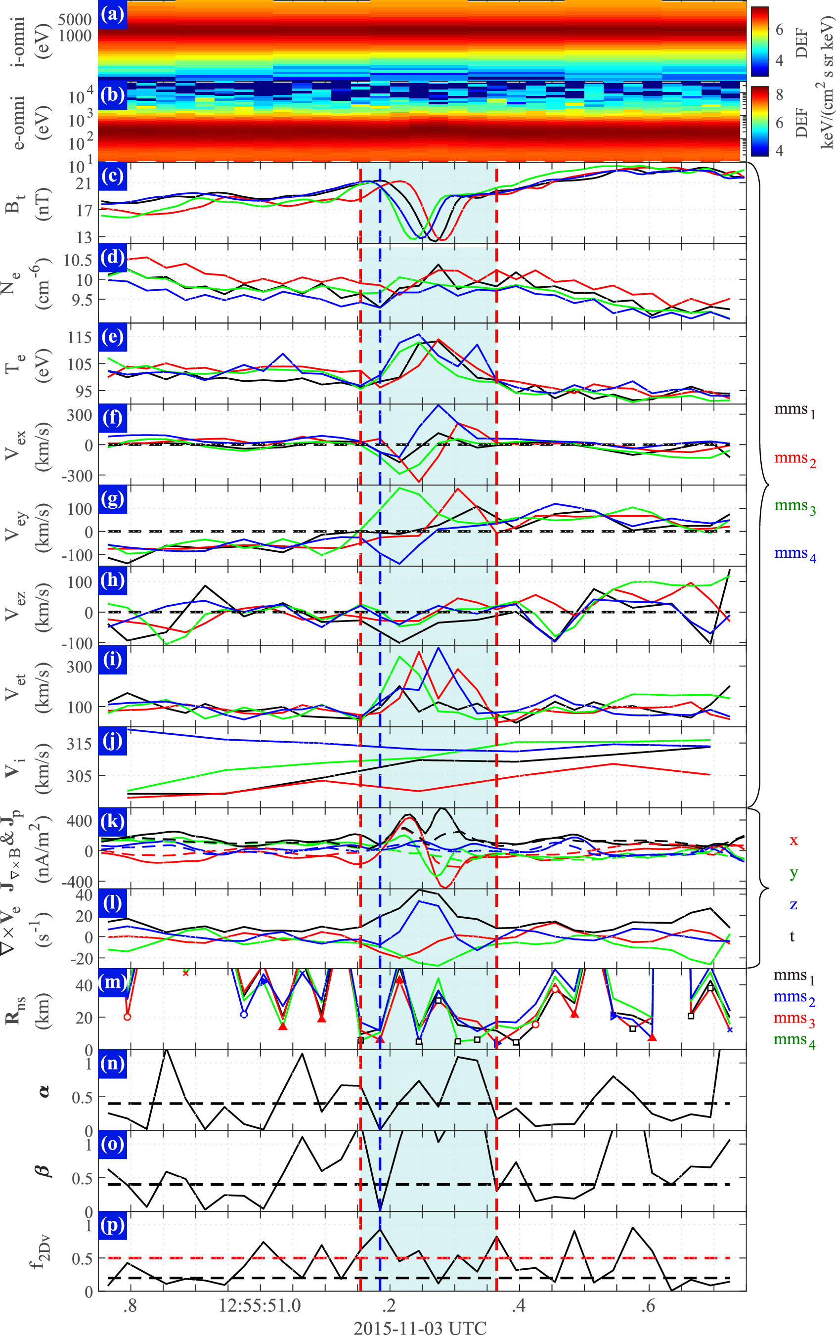
Figure 3. MMS measurements of the event on 2015 November 3 (Case 2) and the results of the identification of velocity nulls using the FOTE-V method. The panels are in the same format as Figure 1.
Download figure:
Standard image High-resolution imageFigures 3(f)–(i) show three components and the total magnitude of electron velocity Vex, Vey, Vez, and Vet, respectively, which are subtracted from the background Veb (i.e., ∼[−7.5, 222.2, −10.1] km s−1). The X-component Vex of the four spacecraft all display an apparent bipolar variation, indicating that all four spacecraft might cross an electron vortex. As can be seen from Figure 3(k), the current densities also show a bipolar variation, both for the curlometer current J∇×B and plasma current Jp . The vorticity of the electron velocity in Figure 3(l) shows a max value of ∼44.1 s−1 in the center of the hole. Then, we use the FOTE-V method to identify the null types during this event and the results are shown in Figure 3(m). The minimum Rns are mainly within the limitation (less than 1 di , ∼73 km) during the MH interval. Figures 3(n) and (o) show two dimensionless parameters α and β to estimate the accuracy of identifying the null properties, with 0.4 as the confidence threshold (the black horizontal dashed lines). As seen from these three panels, the null types are almost unknown (black empty square) with α and β > 0.4 above the dashed line. The few points with reliable α and β < 0.4 are of the spiral types, consistent with the observations of electron vortex. The parameter f2Dv in Figure 3(p) indicates that the electron vortex here is likely a three-dimensional structure with f2Dv > 0.5.
We chose the null point at 12:55:51.185 UT (the vertical dashed blue line in Figure 3) to reconstruct the velocity field topology, with the values of α and β being 0.78% and 1.45%, respectively, which both satisfy the constraints of 40%. First, the eigenvector coordinate system [e1, e2, e3] is obtained based on the Jacobian matrix δ V at the null point: e1 = [0.7303, −0.5686, −0.3786]; e2 = [0.0378, 0.5870, −0.8087]; and e3 = [0.6821, 0.5763, 0.4502] in GSM coordinates. Then, the flow velocities are transferred to the new system and then reconstructed by the formula V ( r ) = ∇ V · ( r − r n) = ∇ V · d R n and the truncated operation based on the spacecraft measurements. The results of the reconstruction are shown in Figure 4, in the same format as Figure 2. Figure 4(a) shows the reconstructed 3D vortex topology with the truncated operation under the reconstruction coordinate system and Figure 4(b) displays the sliced 2D velocity distribution in the fan plane. A distinct vortex null can also be seen both in the 3D and 2D panels. The quivers in Figure 4(b) around the center all point into the null, indicating a flow-in spiral null, consistent with the null type (As) shown in Figure 2(m). Figures 4(c)–(f) display the reconstructed velocities (dashed lines) and observed velocities (solid lines) from 12:55:51.135–12:55:51.235 UT, centered around 12:55:51.185 UT. The reconstructed velocities show little difference from the observed ones. Overall, the analyses for these two cases indicate that MMS successfully detected the electron vortex, and the topologies of the electron flow field in the electron vortex are reconstructed by the FOTE-V method reliably.

Figure 4. The topology of the reconstruction of the velocity vortex center and the results of the comparison for Case 2 in the same format as Figure 2.
Download figure:
Standard image High-resolution image
4. Discussion and Summary
In Section 3, we demonstrated that there exactly exists an electron vortex for both MH events and successfully reconstructed the topology structures of their electron velocity field. Furthermore, we try to estimate the spatial scales of these two vortices.
First, we take the first case as an example. Based on the assumption that the vortex structure is coupling with the background plasmas at the ambient velocity, one can roughly estimate the scales of the vortex LV based on the starting and ending time of the bipolar variations in the electron velocity components through the spacecraft measurements, according to the formula LV = DtV × Vibt. Here Vibt is the ion background velocity, and DtV denotes the time interval corresponding to the variation. The spatial scales turn out to be: LV1 = ∼130.6 km. As for the scales of the vortex for the reconstructed structure, considering the ellipsoid topology in the fan plane displayed in Figures 2(a) and (b), we try to estimate the scales along the short axis and the long axis of the vortex, respectively, for reference. Calculating based on the results of the reconstruction, the scales along two axes when Vet = 0 correspond to the boundary of the vortex LV1' are ∼[88.2, 153.2] km. The same calculation is then carried out for the second case. The vortex scale estimated from the measurements is LV2 = DtV2 × Vibt2 = ∼ 55.6 km. The scales of the reconstructed vortex along the short and long axes of the ellipsoid topology are LV2' ∼ [115.6, 307.6] km corresponding to Vet = 0. Considering the slight deviations in these two scales, it might be connected with the truncated operations, which are determined simply by the vorticity ratio between the center and the background and may not accurately represent the actual situation in the flow nulls. However, these two scales are still in the order of the proton gyroradius. Thus, we prefer to conclude that the reconstruction of the flow velocity can be considered reliable.
With regard to the differences between the reconstructed velocities and measured ones, as shown in Figures 2 and 4, qualitative analysis for the differences and errors in the results of the reconstruction are described below. First, the time resolution of the measured velocities (30 ms for the electrons) may not be high enough for a precise reconstruction, especially for the second case with shorter durations (0.12 s). Besides, the accuracy of the reconstruction may also depend on the configuration as the satellites pass through the vortex structures. The truncated operation in the reconstruction may also lead to some differences, as described above. In addition, the reconstruction method is used based on some assumptions, which may not fit perfectly in the observations, and result in errors.
Furthermore, considering the magnetic field structures, the electron vortex appears with a KSMH in both events. Previous studies suggest the electron vortex be one of the possible mechanisms of the KSMHs (Haynes et al. 2015; Huang et al. 2017b, 2021). However, whether the vortex excites the MH or the MH leads to the vortex is confusing now. As discussed above, the scale of the KSMH is about 86.8 and 37.0 km, respectively. Comparing the scale of the magnetic depression structure and the reconstructed flow structure in the two cases, it seems that the magnetic depression might have a connection with the electron vortex. More investigations in both simulations and observations are needed in the future. Besides, apart from the FOTE-V method developed to reconstruct the three-dimensional plasma velocity fields around the flow null points, several methods of magnetic field reconstruction have also been developed, especially with the high-resolution four spacecraft measurements of the MMS mission. In the early stage, reconstructions of magnetic field topology are based on the typical Grad–Shafranov method (Sonnerup & Guo 1996; Sonnerup & Hasegawa 2011), using one or two spacecraft measurements. Later, the spherical expansion method (He et al. 2008) and the first-order Taylor expansion method (Fu et al. 2015) are put forward to reconstruct the magnetic field topology around magnetic nulls, based on the four spacecraft measurements. Recently, Liu et al. (2019) proposed a new method named the second-order Taylor expansion (SOTE) method, based on the eight-point measurements of magnetic fields and particles. SOTE has been used for the reconstruction of electron-scale MHs both in the magnetosheath and solar wind (Liu et al. 2020). Their results show that the electron-scale MHs may have complex cross-section shapes and short extension lengths along the magnetic field lines, which are inconsistent with the cylinder or planar structures for an MH in previous studies (Haynes et al. 2015; Sundberg et al. 2015). In future work, these reconstruction methods could be combined and utilized to analyze the magnetic field topology and flow-field topology together, to help understand the properties, topologies, and mechanisms of the MHs and electron vortices.
In summary, we have utilized the FOTE-V method to successfully identify electron vortices in space plasmas and reconstruct the topology of their electron flow. The application of this reconstruction method can obviously help improve our understanding of the three-dimensional velocity structures in space and further promote the study of plasma turbulence.
Acknowledgments
This work was supported by the National Key R&D Program of China (grant No. 2022YFF0503700), the National Natural Science Foundation of China (42074196, 41925018), and the China National Postdoctoral Program for Innovative Talents (BX20220238). S.Y.H. acknowledges the project supported by the Special Fund of Hubei Luojia Laboratory.
Data Availability
MMS data is publicly available from NASA's Space Physics Data Facility (SPDF) at https://spdf.gsfc.nasa.gov/pub/data/mms/.