


Abstract
With the growing number of gravitational wave (GW) detections and the advent of large galaxy redshift surveys, a new era in cosmology is emerging. This study explores the synergies between GWs and galaxy surveys to jointly constrain cosmological and GW population parameters. We introduce CHIMERA, a novel code for GW cosmology combining information from the population properties of compact binary mergers and galaxy catalogs. We study constraints for scenarios representative of the LIGO-Virgo-KAGRA O4 and O5 observing runs, assuming to have a complete catalog of potential host galaxies with either spectroscopic or photometric redshift measurements. We find that a percent-level measurement of H0 could be achieved with the best 100 binary black holes (BBHs) in O5 using a spectroscopic galaxy catalog. In this case, the intrinsic correlation that exists between H0 and the BBH population mass scales is broken. Instead, by using a photometric catalog the accuracy is degraded up to a factor of ∼9, leaving a significant correlation between H0 and the mass scales that must be carefully modeled to avoid bias. Interestingly, we find that using spectroscopic redshift measurements in the O4 configuration yields a better constraint on H0 compared to the O5 configuration with photometric measurements. In view of the wealth of GW data that will be available in the future, we argue the importance of obtaining spectroscopic galaxy catalogs to maximize the scientific return of GW cosmology.
Export citation and abstract BibTeX RIS

Original content from this work may be used under the terms of the Creative Commons Attribution 4.0 licence. Any further distribution of this work must maintain attribution to the author(s) and the title of the work, journal citation and DOI.
1. Introduction
Gravitational waves (GWs) emitted by merging compact binaries can serve as standard sirens (Schutz 1986) as their signal provides a direct measurement of the luminosity distance. This makes GWs a new and powerful cosmological probe for tracing the expansion history of the Universe and testing the validity of general relativity on cosmological scales. First of all, the measurement of the expansion history is a longstanding challenge in the field. The discovery of a discrepancy between the value of the Hubble constant H0 measured from the local distance ladder (e.g., Riess et al. 2022) and the one inferred from the cosmic microwave background assuming a ΛCDM cosmology (Planck Collaboration 2020) motivated a rising interest within the community in developing alternative and emerging cosmological probes (see Moresco et al. 2022, for a recent review). Besides being self-calibrated distance tracers, GWs are a particularly promising candidate due to the expected rapid increase in the rate and redshift range of the available catalogs with current and next-generation detectors (Baibhav et al. 2019; Iacovelli et al. 2022a; Branchesi et al. 2023). While the measurement of H0 is driven by low-redshift events, those at redshifts  and beyond open the possibility of testing the distance–redshift relation in full generality. This allows to constrain the dark energy sector, notably, the phenomenon of modified GW propagation (Belgacem et al. 2018a, 2018b; Amendola et al. 2018; Lagos et al. 2019), which is a general prediction of models modifying general relativity at cosmological scales (Belgacem et al. 2019).
The peculiarity of GW cosmology is that determining the redshift with GW data alone is not possible because of its inherent degeneracy with binary masses. External information is required to provide cosmological constraints. 8
A direct measurement of the redshift is possible in the case of a bright siren, i.e., an event with the coincident detection of an electromagnetic (EM) counterpart and the consequent identification of the host galaxy, which allows the redshift to be directly measured from spectroscopy (Schutz 1986; Holz & Hughes 2005; Nissanke et al. 2010; Chen et al. 2018). Such events are rare, as they typically require mergers involving at least one neutron star and a coincident detection of the EM emission. So far, only the binary neutron star (BNS) event GW170817 has an associated counterpart, the gamma-ray burst GRB 170817A (Abbott et al. 2017a, 2017b), which led to the identification of the host galaxy and the first standard siren measurement of H0 (Abbott et al. 2017c), while being a too low redshift to provide a stringent constraint on modified GW propagation (Belgacem et al. 2018b). Detection rates for the ongoing and upcoming observing runs of the LIGO-Virgo-Kagra (LVK) Collaboration are quite uncertain but in general not optimistic (Colombo et al. 2022, 2023).
The largest fraction of events is instead made of binary black holes (BBH) without EM counterparts, known as dark sirens. Using these sources for cosmology has recently become a concrete option with the latest LVK data (Abbott et al. 2021b, 2023a). Two techniques have been primarily employed. The first consists of statistically inferring the redshift from potential host galaxies within the GW localization volume (Schutz 1986; Del Pozzo 2012; Chen et al. 2018; Gray et al. 2020; Gair et al. 2023). 9 This led to measurements of the Hubble constant from LVK data in conjunction with the GLADE (Dálya et al. 2018) and GLADE+ (Dálya et al. 2022) galaxy catalogs (Fishbach et al. 2019; Abbott et al. 2021a; Finke et al. 2021; Gray et al. 2022; Abbott et al. 2023b), as well as the Dark Energy Survey (DES; Soares-Santos et al. 2019; Palmese et al. 2020), the DESI Legacy Survey (Palmese et al. 2023), the DECam Local Volume Exploration Survey (Alfradique et al. 2024) and DESI (Ballard et al. 2023). This method also led to the first dark siren bound on modified GW propagation (Finke et al. 2021). Forecasts indicate that this technique can lead to percent-level measurements with future GW experiments such as LISA (Laghi et al. 2021; Liu et al. 2023), the Einstein Telescope, and Cosmic Explorer (Muttoni et al. 2022, 2023).
Alternatively, the degeneracy between mass and redshift can be broken by modeling intrinsic astrophysical properties as the source-frame mass distribution. In particular, this is possible with spectral sirens—sources whose source-frame mass distribution contains features such as breaks, peaks, or changes in slope (Chernoff & Finn 1993; Taylor et al. 2012; Farr et al. 2019; Mastrogiovanni et al. 2021a; Ezquiaga & Holz 2022). This method allowed in particular to obtain constraints on H0 (Abbott et al. 2023b) and on modified GW propagation (Ezquiaga 2021; Leyde et al. 2022; Mancarella et al. 2022; Magaña Hernandez 2023) from the presence of a mass scale in the BBH distribution (Abbott et al. 2021c, 2023c).
Multiple pipelines have been publicly released, both for the correlation with galaxy catalogs (gwcosmo, Gray et al. 2020; DarkSirensStat, Finke et al. 2021; cosmolisa, Laghi & Del Pozzo 2020) and for spectral sirens (icarogw, Mastrogiovanni et al. 2021b; MGCosmoPop, Mancarella et al. 2022). However, it is known that these two techniques are, in fact, special cases of a unique concept: incorporating prior knowledge about the population in a comprehensive analysis of the ensemble of GW sources (Mastrogiovanni et al. 2021a; Finke et al. 2021; Moresco et al. 2022; Abbott et al. 2023b). Since population properties are known in the source frame (mass and redshift), while GW signals are only sensitive to detector frame quantities (detector frame mass and luminosity distance), the cosmology-dependent mapping between the two allows breaking the mass-redshift degeneracy statistically. In the two aforementioned cases, the population prior used has been either a redshift distribution constructed from a catalog of galaxies, or a model of the source-frame mass distribution. It is natural to seek a unified approach. Moreover, it has been largely recognized that the correlation with a galaxy catalog actually relies on assumptions about the population model for GW sources, and in particular, of a source-frame mass, redshift, and spin distribution (Mastrogiovanni et al. 2021a; Finke et al. 2021; Abbott et al. 2023b). These are needed in particular to consistently account for selection effects, i.e., the fact that not all GW sources are equally likely to be observed. Moreover, an implicit assumption on the mass, redshift, and spin distributions is inherently present in the form of Bayesian priors adopted in the analysis of individual events, and some assumption has also to be used when accounting for the (in-)completeness of the galaxy catalog. These two facts actually make mandatory a joint analysis of the population properties of compact objects and of the cosmological parameters. Doing so while also incorporating the galaxy catalog information is however particularly costly, and until very recently, the population properties of GW sources (and in particular their source-frame mass distribution) have been kept fixed when including the galaxy catalog data.
While this paper was in preparation, two pipelines implementing the joint population and cosmological inference including a galaxy catalog were presented in Mastrogiovanni et al. (2023) and Gray et al. (2023), namely, icarogw2.0 and gwcosmo2.0, building on the homonyms aforementioned codes. Their application to the GWTC-3 catalog (Abbott et al. 2023a) with the GLADE+ galaxy catalog (Dálya et al. 2022) led to updated and more robust measurements of the Hubble constant, as well as of the parameters describing modified GW propagation (the latter being further constrained in Chen et al. 2024), and of alternative cosmological models (Raffai et al. 2024). A machine-learning-based approach has also been proposed by Stachurski et al. (2023).
In this paper, we present and release CHIMERA 10 (Combined Hierarchical Inference Model for Electromagnetic and gRavitational wave Analysis), a novel, independent Python code for the joint analysis of GW transient catalogs and galaxy catalogs. CHIMERA is built starting from DarkSirensStat (Finke et al. 2021) and MGCosmoPop (Mancarella et al. 2022) and allows for the joint inference of cosmology and population properties of GW sources. This paper is associated with version v1.0.0, which is archived on Zenodo (Borghi et al. 2024).
Currently, the information that can be extracted from data with the combined method just described is limited by the lack of a sufficient number of GW events with small enough localization regions and covered by a complete galaxy catalog. In order to fully appreciate the gain achievable from this method, it is therefore of interest to study its potential with upcoming GW data combined with a complete galaxy catalog. This will become a concrete possibility in the coming years, thanks to galaxy surveys already in the data release stage such as DESI (DESI Collaboration et al. 2016), and in the data acquisition period such as that of Euclid (Laureijs et al. 2011). In this context, it is also important to understand how large the impact of the redshift measurement uncertainties can be and to assess the relative importance of the information coming from the galaxy survey and from the population model, respectively. This is the second goal of the paper, where we explore for the first time the application of this technique in the context of future GW observations and study in detail the impact of different galaxy catalog properties. We focus here in particular on the measurement of the Hubble constant. We simulate GW detections with detector networks and sensitivities corresponding to the ongoing "O4" run of the LVK collaboration, as well as of the future "O5" observing run. We study the constraining power of the best 100 events observed in 1 yr, considering a complete galaxy catalog with both spectroscopic and photometric uncertainties on the galaxies' redshifts (for a study of the limited impact of different assumptions on the shape of galaxy redshift uncertainties with current data, see Turski et al. 2023). We also compare to the case where no information from the galaxy catalog is present.
The paper is organized as follows. In Section 2, we present the statistical framework and its implementation in CHIMERA. In Section 3, we describe the generation of mock galaxy and GW catalogs. Section 4 provides results for both the O4- and O5-like scenarios. Finally, Section 5 concludes the paper and discusses future applications of this method.
2. Statistical Framework
We consider a population of GW sources, individually described by source-frame parameters
θ,
which globally follow a probability distribution ppop(
θ
∣
λ
) described by hyperparameters
λ
. We summarize here the hierarchical Bayesian inference formalism to infer
λ
given a catalog of GW detections and a catalog of their potential hosts with measured redshifts.
11
We separate the hyperparameters describing the underlying cosmology
λ
c (e.g., H0, Ωm) from the ones describing the astrophysical population of GW sources, as the mass distribution
λ
m (e.g., the mass scale, see Section 3.2.2) and redshift distribution
λ
z (e.g., the peak of cosmic star formation, see Section 3.2.1), so that
λ
= {
λ
c,
λ
m,
λ
z}
12
. In this work,
λ
m,
λ
z, and
λ
c are considered to be independent of each other. Given a set  (i = 1,...,Nev) of data from independent GW events, the population likelihood is (Mandel et al. 2019; Vitale et al. 2022),

where  is the individual source likelihood and

is the selection function, which corrects for selection effects (Loredo 2004; Mandel et al. 2019). When ppop(
θ
∣
λ
) is correctly normalized to unity, ξ(
λ
) measures the overall fraction of detectable events given
λ
.  gives the probability of detecting an event with parameters
θ
. We consider the following set of source parameters:
gives the probability of detecting an event with parameters
θ
. We consider the following set of source parameters:  , where z is the redshift of the binary,
  the sky localization, and m1, m2 are the primary and secondary masses.
Note that, when the cosmological hyperparameters
λ
c are included in the analysis, the single-event GW likelihood written in source-frame variables in Equation (1) includes an explicit dependence on
λ
c. This is a consequence of the fact that GW observations do not provide information on source-frame parameters, but on detector frame quantities  . Those are then mapped to the source frame in a way that depends on the underlying cosmology. Explicitly, the source-to-detector frame conversion requires inverting the relations


where dL is the luminosity distance, which, in a flat ΛCDM cosmology, is given by

with λ c ≡ {H0, Ωm,0} and the Hubble parameter being

where the radiation is not considered as its contribution is negligible in the late Universe. Alternatively, Equation (1) could be written in the detector frame to remove the dependence on
λ
c (see Finke et al. 2021 for a detailed discussion). In this work, for the actual implementation, we find it more convenient to work in a source frame, as will be clear below—essentially, this is due to the fact that the galaxy catalog is naturally given in redshift space. Note that the single-event GW likelihood is a probability distribution normalized on the data, not on the parameters, so in the transformation from
θ
to  it remains unchanged. However, in practical applications of hierarchical inference, we are provided with a set of samples drawn from the posterior distribution
  for each event in the GW catalog, obtained with priors
  . It is thus convenient to reexpress the single-event GW likelihood via Bayes' theorem as
  . The posterior
  can then be obtained from the (cosmology-dependent) conversion of the posterior samples of
  to the source frame, while the prior π(
θ
i
) is related to the one in the detector frame by
to the source frame, while the prior π(
θ
i
) is related to the one in the detector frame by  . Explicitly, for the variables of interest here, the Jacobian factors are given by

Finally, under the assumption that the mass function does not evolve with cosmic time, 13 the population function can be split as follows:

where  denotes the direction in the sky. In the subsequent sections, we will describe in detail the construction of the population prior to taking into account a galaxy catalog and the source-frame mass distribution of the population of compact binaries.
2.1. Redshift Prior
The core of the method is the construction of a population prior on the GW source redshift from a galaxy catalog. This is given by the second term of Equation (8) that we factorize as follows:

where pgal is the probability that there is a galaxy at ( ) and prate the probability of a galaxy at redshift z to host a GW event. This takes into account that the probability for a galaxy to host a merger can have a nontrivial redshift dependence. We assume that this can be parameterized as

where ψ(z; λ z) is the merger rate evolution of compact objects with redshift and the term (1 + z)−1 takes into account the conversion between source and detector time. Note that the normalization integral in Equation (9), as well as any rate normalization factor in Equation (10), simplifies between numerator and denominator in Equation (1) and does not need to be computed explicitly.
2.2. Galaxy Catalog
As a first approximation, we assume to have a complete galaxy catalog, i.e., this contains all the potential host galaxies. In this case, we denote as  the probability distribution built from galaxies in the catalog. We can write
  and compute the latter probability as a sum over the contribution of each galaxy. Given a set of
  (g = 1,...,Ngal) EM observations of galaxies we have

where wg
weights the probability of each galaxy to host a GW event (e.g., by the galaxy luminosity),  is the galaxy's redshift distribution that we want to use as a prior, and
  is a Dirac delta distribution of each galaxy's sky localization that can be treated as errorless.
The galaxy catalog contains redshift measurements  and associated uncertainties
  for each observed galaxy, i.e.,
  . From these quantities, we construct the likelihoods, which we assume to be Gaussian,
  . This is a probability distribution over the observed values
  . To get
  we need to multiply it by a prior on the redshift distribution, which in the absence of other information is naturally chosen as uniform in comoving volume (Gair et al. 2023). Using Bayes' theorem, we get

where dVc
/dz is the differential comoving volume element in a flat universe. With this definition, Equation (11) is normalized so that if  and in case of uniform weights, we get
  , which is consistent with Equation (3.39) of Finke et al. (2021), i.e., the comoving density of galaxies ncat(z) is estimated by counting the objects in the catalog and dividing by the total volume. If, instead, the likelihood is completely uninformative,
  , we correctly get a comoving density constant in redshift. Note that the assumption of a uniform-in-comoving-volume prior introduces a dependence on the cosmology in the redshift prior, since dVc
/dz is a function of
λ
c. Once normalizing correctly
, we correctly get a comoving density constant in redshift. Note that the assumption of a uniform-in-comoving-volume prior introduces a dependence on the cosmology in the redshift prior, since dVc
/dz is a function of
λ
c. Once normalizing correctly  , however, the dependence on H0 cancels, as this is an overall multiplicative factor in dVc
/dz, but a dependence on Ωm,0 remains and should be accounted for. The same would be true if one wished to include more general cosmologies, e.g., a Dark Energy equation of state wDE ≠ −1. Alternatively, one may adopt a flat prior, which eliminates the extra dependence on the cosmology, as done, e.g., in Gray et al. (2023).
, however, the dependence on H0 cancels, as this is an overall multiplicative factor in dVc
/dz, but a dependence on Ωm,0 remains and should be accounted for. The same would be true if one wished to include more general cosmologies, e.g., a Dark Energy equation of state wDE ≠ −1. Alternatively, one may adopt a flat prior, which eliminates the extra dependence on the cosmology, as done, e.g., in Gray et al. (2023).
In the real world, observed galaxy catalogs are subject to selection effects that result in having an incomplete set of potential hosts. To address this issue, the pgal term in Equation (9) has to be modified including the probability of missing galaxies,  , as follows (Chen et al. 2018; Finke et al. 2021):

The probability  is constructed with two pieces of information. The first is the number of missing galaxies as a function of redshift and sky position, encoded in the completeness fraction of the catalog
  . This can be estimated with some assumption on the total comoving density of galaxies or on the luminosity distribution of a complete sample that is assumed to follow a Schechter function. We refer to Finke et al. (2021) for a rigorous definition of this quantity and for the discussion of different ways to compute it. In CHIMERA, we will use in particular the so-called mask completeness of Finke et al. (2021), which we will describe better in Section 2.4. From this, one can compute the weight
  in Equation (13) as

where the integral extends to a region sufficiently large to encompass all the GW events under consideration and Vc ( λ c) denotes the corresponding comoving volume.
The second bit of information amounts to specifying how the missing galaxies are distributed. Two extreme possibilities are a homogeneous completion, where the distribution is assumed to be uniform in comoving volume and sky position, and a multiplicative completion, where missing galaxies are assumed to trace the distribution of those present in the catalog (Finke et al. 2021). The two correspond to


In practice, as suggested in Finke et al. (2021) and done in the code DarkSirensStat, it is convenient to interpolate between a multiplicative completion where the catalog is fairly complete, and a homogeneous completion where the catalog is largely incomplete. Finally, an even better option, suggested in Finke et al. (2021) and recently studied in detail in Dalang & Baker (2024), would be to complete the catalog using the typical correlation length of galaxies.
2.3. Full Form of the Likelihood
By putting together Equations (1)–(14) we can write the likelihood in its final form. In the following, we explicitly restrict to the subset of source parameters  and
and  . This relies on the assumption that the remaining parameters of the GW waveform (see Equation (27) below) have a population distribution that coincides with the prior used in the analysis of individual events. We have


Note that we have omitted the overall normalization of the redshift prior, as this is independent of  and is present also in the selection function, leading to a simplification between numerator and denominator in Equation (17). A different normalization of this quantity just amounts to a different interpretation of the selection function, which does not correspond to the fraction of detectable events, as a consequence of the fact that ppop loses its correct normalization to unity. We find the form of Equations (17)–(19) useful since it makes clear what quantities actually need to be computed in the numerical evaluation. On the other hand, we note that the normalization of the term pgal has to be computed carefully, in order to correctly balance the contributions of the catalog and missing terms in Equation (13).
2.4. Implementation in CHIMERA
We now discuss the implementation of the method in CHIMERA. The code accurately computes Equation (17) across different regimes, i.e., when the EM redshift information in highly constraining (bright sirens), more loosely constraining (dark sirens), or not present at all (spectral sirens). We also prioritize computational efficiency to meet the demands of next-generation GW observatories and upcoming galaxy surveys.
In this section, we summarize the key aspects of the code, while a more detailed description is provided in Appendix A. We will use the real event GW170817 as an illustrative example, considering it a dark siren in conjunction with the GLADE+ galaxy catalog. This is useful because GW170817 is the best-localized GW event so far and its host galaxy, NGC 4993, has been uniquely identified (Abbott et al. 2017a), providing an ideal benchmark for dark siren techniques. Indeed, this is often used as a test case and allows comparison to other pipelines (Mastrogiovanni et al. 2023, Gray et al. 2023). In Appendix B, we provide details about the data and cuts used for this example.
Figure 1 shows a compact representation of the workflow of CHIMERA, in the case of GW170817. In short, the galaxy catalog term is precomputed as a function of redshift (red lines) on a pixel-by-pixel basis inside the GW localization region (given by the gray squares). The GW kernel in Equation (18) is given by a kernel density estimation (KDE) of the GW posterior samples reweighted for the population prior on source-frame masses (blue area).

Figure 1. Visual representation of the underlying workflow of CHIMERA. The GW probability is approximated by a three-dimensional KDE  , while the galaxy probability pgal is evaluated by summing the individual galaxy's contributions within the pixel enclosed in the GW sky localization area.
Download figure:
Standard image High-resolution image
Pixelization and precomputation of the galaxy term. The quantity  can be cosmology dependent, but only when adopting a cosmology-dependent prior on the galaxies' redshifts, and in any case never on H0, as explained in Section 2. If adopting a flat prior on the galaxies' redshifts, or a narrow prior on the other cosmological parameters (e.g., a Planck prior on the matter density), the quantity pgal can be computed once for all, given a specific galaxy catalog. For each event in the GW catalog, CHIMERA selects galaxies enclosed in the GW localization volume, with a redshift range computed taking into account all of the prior range for H0. Then, the sky area of the GW event is divided into equal-area pixels in the pixelization scheme of Healpix (Górski et al. 2005; Zonca et al. 2019). CHIMERA includes an adaptive pixelization procedure that allows to set the pixel size for each GW event depending on its localization area (see Appendix A for details). This step corresponds to the left panel of Figure 2, where we show the galaxies enclosed in the 90% localization volume of GW170817 as red crosses, overlapping the pixels. The quantity
  is then approximated as a redshift-dependent function of the form given in Equations (11) and (12) for each pixel, by summing the contribution of all the galaxies enclosed within it. The weights in Equation (11) can be chosen to be either uniform or corresponding to the galaxies' luminosity in the catalog. The redshift distributions in each pixel are shown in red in the central panel of Figure 2 for the example of GW170817. This method allows for the compression of the information coming from all galaxies in each pixel in a single function of redshift. In the case of GW170817, we find 88 galaxies in the 90% localization volume, while using 20 pixels, which corresponds to a factor of ∼5 improvement in the computational cost. This procedure is even more effective in the case of events with thousands of galaxies in the localization region. We note that, in general, the GW sky map changes on much larger angular scales than the galaxy distribution. This means that the compression introduced here (which basically amounts to approximating the galaxies' angular positions with the center of each pixel) does not lead to a loss of information as far as the pixel size is chosen appropriately.

Figure 2. Analysis of GW170817 with CHIMERA using GLADE+ galaxies with a luminosity  . Left: sky distribution of the potential host galaxies (red crosses) contained in the 90% credible pixels (gray squares). The true host NGC 4993 is identified with a gold circle. Center: redshift distribution of the GW kernel (blue) assuming H0 = 70 km s−1 Mpc−1 and galaxy probability pgal (red) in each pixel. The pixel including NGC 4993 is colored in black. Right: posterior distributions on H0 assuming that the true host is or is not observed.
Download figure:
Standard image High-resolution image
Catalog completeness. The completeness fraction  is computed following the mask method presented in Finke et al. (2021). First, similar pixels are grouped together in masks by applying an agglomerative clustering algorithm. The chosen feature for this purpose is the number of galaxies within each pixel. The number of masks is arbitrarily chosen depending on the survey properties. For each mask, the completeness fraction is computed by comparing the luminosity function at each redshift to a reference Schechter function. We refer to Finke et al. (2021) for a more detailed description of this procedure. In particular, this allows us to easily cut regions particularly under-covered by the galaxy survey, for example, the region of the sky covered by the Milky Way. It also makes straightforward use of galaxy catalogs with partial sky coverage. In the example of GW170817, it is complete.
3D GW kernel. We now turn to the term  in Equation (18). For each GW event, we have a set of posterior samples of the detector frame quantities
  approximating the posterior probability
  . CHIMERA assumes that the prior on detector frame masses used for the individual event analysis is flat,
  , while the prior on the luminosity distance is
  . Then, for each value of
λ
, the samples are converted to source-frame quantities by inverting Equations (3)–(5). Each sample, labeled by j, is assigned a weight equal to
. Then, for each value of
λ
, the samples are converted to source-frame quantities by inverting Equations (3)–(5). Each sample, labeled by j, is assigned a weight equal to

and  is obtained by a 3D weighted KDE in the space (z, R.A., decl.) with weights
  . Using the reweighted samples in this subspace corresponds to performing the integral in Equation (18) with the correct population prior p(m1, m2 ∣
λ
m) on the source-frame masses. This will encode a dependence on the cosmological parameters, which enters in the conversion of the posterior samples from the detector frame to the source frame, resulting in a reshaping of the kernel
. Using the reweighted samples in this subspace corresponds to performing the integral in Equation (18) with the correct population prior p(m1, m2 ∣
λ
m) on the source-frame masses. This will encode a dependence on the cosmological parameters, which enters in the conversion of the posterior samples from the detector frame to the source frame, resulting in a reshaping of the kernel  . A nonflat source-frame mass spectrum will add redshift information at the statistical level through this term, even in the absence of a galaxy catalog, in which case we recover the spectral siren case. For GW170817, the GW kernel is plotted in blue in Figure 2(central panel), assuming a value of H0 = 70 km s−1 Mpc−1 and a flat mass distribution between 1 and 3 M☉
Integration. The double integral in Equation (17) is performed by integrating numerically dz in each pixel first. Then, the integral in  can be approximated as a discrete sum of the results in each pixel, multiplied by the pixel area. The latter, for each given GW event, is equal for all pixels and inversely proportional to the number of Healpix pixels of the map. So, in the end, the angular integral in Equation (17) is obtained as an average over pixels.
Selection effects. The selection bias term ξ(
λ
) from Equation (2) is computed by using the standard reweighted Monte Carlo (MC) method (Tiwari 2018; Farr 2019). In this case, it is crucial to use detector frame quantities, since the detectability in a GW experiment is a function of those only, i.e.,  . This allows us to compute this function only once. The integral in Equation (19) can then be computed with the change of variables
  , where the Jacobian factors are given in Equation (7). CHIMERA takes as input a set of simulated events, each with detector frame parameters
  , drawn from a reference distribution with probability
  . These must have been previously injected in the same detection pipeline used to obtain the GW catalog, storing those that pass the detection threshold.
Then, the selection function in Equation (19) is computed with MC integration as

where Ninj is the total number of injections, Ndet the number of detected ones, and the source-frame quantities zi , m1,i , and m2,i are understood to be computed from the (fixed) detector frame ones via inversion of Equations (3)–(5), and are thus functions of the cosmological parameters λ c. Finally, when computing the selection bias term, CHIMERA employs a galaxy catalog interpolant pgal constructed on the full sky.
Accuracy of the MC integrals. Finally, when computing Equation (21), we ensure that the effective number of independent draws after reweighting, Neff, for a given population is sufficiently high ( , see Farr 2019). This criterion is also applied to the GW kernel weights to ensure numerical stability.
In conclusion, the right panel of Figure 2 shows the results for the posterior probability on H0 (solid line). We obtain a value of  in the dark siren case, in good agreement with Fishbach et al. (2019). As can be seen from Figure 2 (central panel), the primary contribution to the posterior arises from galaxies at approximately z ∼ 0.01. This value combined with the GW measurement of dL
∼ 40 Mpc, implies H0 ∼ 70 km s−1 Mpc−1. The galaxy groups at z ∼ 0.02 (0.04) provide a shallower contribution to H0 ∼ 150 (300)km s−1 Mpc−1 due to the presence of selection effects that disfavor high values of H0
in the dark siren case, in good agreement with Fishbach et al. (2019). As can be seen from Figure 2 (central panel), the primary contribution to the posterior arises from galaxies at approximately z ∼ 0.01. This value combined with the GW measurement of dL
∼ 40 Mpc, implies H0 ∼ 70 km s−1 Mpc−1. The galaxy groups at z ∼ 0.02 (0.04) provide a shallower contribution to H0 ∼ 150 (300)km s−1 Mpc−1 due to the presence of selection effects that disfavor high values of H0
 ]. In this case, the assumption of a population model for GW170817 provides no significant improvements to H0.
For comparison and to test the performance of the code in the bright siren regime, we repeat the analysis assuming the identification of the host galaxy with z = 0.0100 ± 0.0005 (Abbott et al. 2017a). In this case, we assign a weight w = 1 to NGC 4993 and w = 0 to all the other galaxies (see Equation (11)). The resulting posterior on H0 is shown in Figure 2(c) (dashed line). In the bright siren case, we obtain a value of  , in very good agreement with Abbott et al. (2023b).
3. Mock Catalogs
In this section, we describe the procedure to build realistic mock galaxy and GW catalogs. These will be used to both validate the code and provide updated forecasts for O4- and O5-like detector configurations.
3.1. Parent Galaxy Sample
We generate our mock galaxy catalog (hereafter, parent sample) from the MICE Grand Challenge light-cone simulation (v2), which populates one octant of the sky (close to 5157 deg2) designed to mimic a complete DES-like survey up to an observed magnitude of i < 24 at redshift z < 1.4 (Carretero et al. 2015; Crocce et al. 2015; Fosalba et al. 2015a, 2015b; Hoffmann et al. 2015). MICE assumes a flat ΛCDM cosmology with H0 = 70 km s−1 Mpc−1, Ωm,0 = 0.25, and ΩΛ,0 = 0.75.
While we ideally require a complete catalog with high number density, as a simplifying assumption in this paper we consider only galaxies with stellar masses  . This cut is consistent with the idea that the binary merger rate is traced by stellar mass, as also adopted in current standard sirens analysis via absolute magnitude cuts and luminosity weighting (Fishbach et al. 2019; Finke et al. 2021; Gray et al. 2022; Abbott et al. 2023b; Mastrogiovanni et al. 2023; Gray et al. 2023). A similar cut in mass is also considered (Muttoni et al. 2023) in the context of simulations for the Einstein Telescope.
We subsample the MICEv2 catalog to reproduce the density for the cut described above extracting the galaxies to get a uniform in comoving volume distribution. In the end, we obtain a parent sample of about 1.6 million massive galaxies.
For the redshift uncertainties, we consider two cases. First of all, we explore the possibility of maximizing the galaxy catalog information by having a spectroscopic catalog. This could be done by expanding the currently available catalogs (GLADE+ Dálya et al. 2022) in the future by exploiting the information provided by the next large spectroscopic surveys. As an example, the ESA mission Euclid (Laureijs et al. 2011) will provide an all-sky map of spectroscopic redshift in the range of 0.9 < z < 1.8, with an accuracy of σz /(1 + z) ≲ 0.001, and the Dark Energy Spectroscopic Instrument (DESI; DESI Collaboration et al. 2016) is planned to observe ∼14,000 deg2 covering the redshift range of 0.4 < z < 2.1. Second, we study how the information extracted changes when using photometric redshift, assuming an uncertainty σz /(1 + z) = 0.05. This is easily accessible with current ongoing surveys like DES (e.g., DES has reached σz ∼ 0.01 (Myles et al. 2021), and this limit can be pushed to σz ∼ 0.007 with improved techniques, e.g., Buchs et al. 2019) on a smaller area, and in future surveys like Euclid and Rubin Observatory (Ivezić et al. 2019) are planned to extend it to the entire sky to a depth of Euclid H magnitude HE ∼ 24 (HE ∼ 26 in the Deep Survey) and an expected uncertainty σz /(1 + z) ≲ 0.05 (Euclid Collaboration et al. 2020, 2022).
Therefore, in this paper, we consider two regimes of photometric (hereafter, "phot") and spectroscopic (hereafter, "spec") redshift uncertainties:

3.2. Sample of GW Events
We generate mock GW events from the parent sample by fixing cosmological hyperparameters λ c and astrophysical population hyperparameters λ z and λ m. We describe the redshift and mass distributions in turn.
3.2.1. Rate Evolution
The source-frame merger rate is parameterized as follows (see Madau & Dickinson 2014):

where ψ(z) ∝ (1 + z)γ at low z, then reaches its peak near zp, and subsequently declines as ψ(z) ∝ (1 + z)−κ . To build the catalog, we use γ = 2.7 consistent with the LVK GWTC-3 results (Abbott et al. 2023c). The limited detection range of current GW detectors restricts our ability to determine the merger rate at higher redshifts, therefore we adopt zp = 2, κ = 3, consistent with the idea that ψ(z; λ z) follows the galaxy's star formation rate density with parameters from Madau & Dickinson (2014). The catalog of potential sources is then obtained by sampling the parent sample using a weight proportional to the detector frame merger rate ψ(z; λ z)/(1 + z).
3.2.2. Mass Distribution
For the mass distribution, we adopt the phenomenological "PowerLaw+Peak" (PLP) model following the LVK GWTC-3 results (Abbott et al. 2023c). The mass term of Equation (8) is factorized as follows:

The probability of the primary BH mass is given by

where  is a power law truncated in the domain m ∈ [mlow, mhigh],
  is a Gaussian component whose contribution relative to
  is regulated by λg, and
 ![${ \mathcal S }(m)\in [0,1]$](https://content.cld.iop.org/journals/0004-637X/964/2/191/revision1/apjad20ebieqn65.gif) is a smoothing piece-wise function with a tapering parameter δm
fully described in Appendix
is a smoothing piece-wise function with a tapering parameter δm
fully described in Appendix
3.2.3. Summary
With the above assumptions, the cosmological and astrophysical hyperparameters to be studied are

The fiducial values and the prior ranges chosen for this work are reported in Table 1. For the cosmological parameters, we will consider the value of the matter density to be fixed to its fiducial value.
Table 1. Summary of the Population Hyperparameters and Priors Adopted
| Parameter | Description | Fiducial Value | Prior |
|---|---|---|---|
| Cosmology (flat ΛCDM) | |||
| H0 | Hubble constant [km s−1 Mpc−1] | 70.0 |

|
| Ωm,0 | Matter energy density | 0.25 | Fixed |
| Rate evolution (Madau-like) | |||
| γ | Slope at z < zp | 2.7 |

|
| κ | Slope at z > zp | 3 |

|
| zp | Peak redshift | 2 |

|
| Mass distribution (PowerLaw+Peak) | |||
| α | (Primary) slope of the power law | 3.4 |

|
| β | (Secondary) slope of the power law | 1.1 |

|
| δm | (Primary) smoothing parameter [M⊙] | 4.8 |

|
| mlow | Lower value [M⊙] | 5.1 |

|
| mhigh | Upper value [M⊙] | 87.0 |

|
| μg | (Primary): mean of the Gaussian component [M⊙] | 34.0 |

|
| σg | (Primary): standard deviation of the Gaussian component [M⊙] | 3.6 |

|
| λg | (Primary): fraction of the Gaussian component | 0.039 |

|
Note.
 denotes a uniform distribution.
Download table as: ASCIITypeset image
3.3. GW Data Generation
For the simulation of GW detections, we use the simulation pipeline GWFAST 14 (Iacovelli et al. 2022a, 2022b).
We assume quasi-circular non-precessing BBH systems. Their waveform is characterized by the detector frame parameters

where  is the detector frame chirp mass, η is the symmetric mass ratio, χ1/2,z
are the adimensional spin parameters along the direction of the orbital angular momentum, dL
is the luminosity distance, θ = π/2 − decl. and ϕ = R.A. are the sky position angles, ι refers to the inclination angle of the binary's orbital angular momentum with respect to the line of sight, ψ is the polarization angle, tc
is the coalescence time, and Φc
is the phase at coalescence.
is the detector frame chirp mass, η is the symmetric mass ratio, χ1/2,z
are the adimensional spin parameters along the direction of the orbital angular momentum, dL
is the luminosity distance, θ = π/2 − decl. and ϕ = R.A. are the sky position angles, ι refers to the inclination angle of the binary's orbital angular momentum with respect to the line of sight, ψ is the polarization angle, tc
is the coalescence time, and Φc
is the phase at coalescence.
First of all, we generate a population of GW events following the prescriptions given in Section 3.2, so that each source is characterized by a set of source-frame parameters
θ
. For the parameters in Equation (27) that are not explicitly mentioned in Section 3.2, we assume the following distributions: the sky position angles are uniform on the octant covered by the parent sample, the inclination angles have a uniform distribution in  in the range [0, π], the polarization angle and coalescence phase have a uniform distribution in [0, π] and [0, 2π], respectively, and the time of coalescence, given as Greenwich mean sidereal time and expressed in units of fraction of a day, is uniform in the interval [0, 1]. For the spin parameters instead, we adopt a flat distribution between [−1, 1] for the components aligned with the orbital angular momentum. The source-frame parameters are then converted to a detector frame using the fiducial cosmology (see Table 1).
For each source, we simulate GW emission and compute the network matched-filtered signal-to-noise ratio (S/N) using the IMRPhenomHM (London et al. 2018; Kalaghatgi et al. 2020) waveform approximant, which includes the contribution of subdominant modes to the signal, that are of great relevance to describe in particular the merger phase of BBH systems. We consider two network configurations. The first, denoted as O4-like, is composed of a network of the two LIGO interferometers at Hanford, Washington, and Livingston, Louisiana, USA, the Virgo interferometer in Cascina, Italy, and the KAGRA interferometer in Japan. We assume sensitivity curves representative of the O4 run of the LVK Collaboration, with public sensitivity curves from Abbott et al. (2016). For the second configuration, denoted as O5-like the network includes the two LIGO, Virgo, and KAGRA instruments, as well as a LIGO detector located in India. For O4, we use sensitivity curves representative of the O5 run of the LVK Collaboration 15 (Abbott et al. 2016). We assume a 100% duty cycle in all cases.
Then, we select samples of GW events as follows:
- 1.O4-like: 100 events with a network S/N > 12;
- 2.O5-like: 100 events with a network S/N > 25.
These cuts are designed to yield the 100 best events for each configuration over approximately 1 yr of observation. We determined these numbers simulating with GWFAST a 1 yr observing run for each of the two scenarios, with a population of BBHs with an overall merger rate calibrated on the latest LVK constraints (see, e.g., Iacovelli et al. 2022a). We note that the fact that the simulation is performed on one octant of the sky is irrelevant in our case, as we do not constrain direction-dependent hyperparameters.
We approximate the GW posterior probability with the Fisher information matrix (FIM) approximation, where the GW likelihood  is assumed to be given by a multivariate Gaussian distribution. This approximation is valid for the high S/N events that we are considering in this work (see Iacovelli et al. 2022a for details). We compute the FIM with GWFAST. For each event, we then draw 5000 samples from a multivariate Gaussian distribution with covariance equal to the inverse of the FIM, further imposing priors that are chosen to be flat in detector frame masses with the condition
  ,
,  for the luminosity distance, and equal to the distributions used to sample the events for the remaining parameters. We then use the samples of
  R.A., decl. to compute the GW likelihood as described in Section 2.4.
The main properties of the galaxy and GW catalogs are summarized in Figure 3. The top panels show the GW skymaps of the events detected in the two configurations overlaid to the galaxy sky distribution. The central panels present the scatter plots of the sky localization area versus the error on dL (with a color scale giving information on the S/N). Finally, the bottom panels show the redshift and mass distribution of the detected GW events, as well as the distribution of the number of galaxies found within their localization volumes.

Figure 3. Main properties of the simulated O4-like (blue) and O5-like (red) GW catalogs. Upper panels: GW sky localization areas at 1 and 2σ overlaid to their potential host galaxies (gray) extracted from MICEv2. Middle panels: distribution of the relative uncertainty on the luminosity distance and sky localization area as a function of network S/N. Lower panels: distribution of the GW events as a function of (left to right): redshift, primary mass, and number of galaxies contained in the GW localization volume.
Download figure:
Standard image High-resolution imageThe O4-like events are at redshift z ≲ 0.9 with sky areas between a few and a few hundred square degrees. This typically results in more than ∼500 potential host galaxies for 90% of the events (Figure 3, bottom-right panel). A particularly lucky event is present with a small localization area (∼2 deg2) and high S/N (∼55, see the mid-left panel of Figure 3). While this event represents an outlier of the distribution that can be ascribed to a statistical fluctuation, it still represents a possibility with this configuration. For the O5-like events, the redshift distribution remains limited to z ≲ 1 as a consequence of the higher S/N cut, while the larger and more sensitive detector network substantially improves the localization capabilities. This typically results in more than ∼50 potential host galaxies for 90% of the events (Figure 3, bottom-right panel). In this configuration, there is a significant tail of events with just a few tens of galaxies, corresponding to sky localization regions of less than 1 deg2 with an S/N that can exceed 100. Overall, while the number of galaxies in the localization volume depends on the assumption on the galaxy catalog employed, it is interesting to observe the 10× reduction in the number of potential host galaxies between the O4 and O5 networks. This improvement, following from the much smaller localization volumes, is a key factor in obtaining improved dark siren constraints as discussed in Section 4.
Ultimately, for the computation of the selection bias, we generate injection sets for both the O4-like and the O5-like scenarios with GWFAST, adopting the same selection cuts as for the GW catalogs. The injections cover the same sky area as the catalogs and a distance range that arrives up to the detector horizon for the given S/N cuts. The injection set is made of Ninj = 2 × 10⁷ and 4 × 10⁷ events, resulting in about 1.5 × 10⁶ and 1 × 10⁶ detected events in the O4- and O5-like scenario, respectively. These are then used to estimate the selection bias as in Equation (21).
4. Results
In this section, we report the results of the analyses of the O4- and O5-like configurations. For both detector networks, we consider three distinct analysis setups:
- 1.Full (zspec): Full analysis using the parent catalog of 1.6 million galaxies derived from MICEv2 adopting spectroscopic redshift uncertainties as in Equation (22).
- 2.Full (zphot): Full analysis as above, adopting broader (photometric) redshift uncertainties as in Equation (22).
- 3.Spectral: No galaxy catalog information is incorporated and instead galaxies are assumed to be uniformly distributed in comoving volume. The constraints are based only on the assumption of the source-frame mass distribution.
In this way, we obtain a total of six configurations. We adopt wide uniform priors for all the hyperparameters (Table 1). The posterior distribution is sampled with affine-invariant Markov Chain Monte Carlo sampler emcee (Foreman-Mackey et al. 2013) and the convergence is assessed ensuring that the number of samples is at least 50 larger than the integrated autocorrelation time for all the parameters. Results are reported using the median statistic with symmetric 68.3% credible levels.
The final constraints on all individual parameters are reported in Table 2, while the marginalized posterior distribution for a selection of cosmological (H0), mass (α, μg, σg), and rate (γ) parameters is shown in Figure 4. In Figure 5, we show the relative uncertainty on H0 in all configurations. Finally, in Appendix D we show an example of the full corner plot. For all the six configurations, with CHIMERA we recover the fiducial values with a typical deviation of 0.2 σ, with fluctuations that can be ascribed to the specific realizations of the data sets.

Figure 4. Marginalized posterior distributions of a selection of hyperparameters in the O4-like (upper panels) and O5-like (lower panels) detector networks. The analysis is performed with CHIMERA in three setups, namely, spectral-only (Spect.) and spectral with the inclusion of a photometric (zphot) or spectroscopic (zspec) galaxy catalog.
Download figure:
Standard image High-resolution image
Figure 5. Relative uncertainty on H0 obtained from spectral-only and full standard sirens analysis of 100 BBHs in the O4- and O5-like network configurations, including a complete galaxy catalog with photometric or spectroscopic redshift uncertainties.
Download figure:
Standard image High-resolution imageTable 2. Median and 68% Confidence Level Interval of the Hyperparameters Resulting from Spectral-Only and Full Analyses for the O4- and O5-like Configurations and for Spectroscopic and Photometric Errors on the Galaxy Redshifts
| O4-like (100 Events with S/N > 12) | O5-like (100 Events with S/N > 25) | |||||
|---|---|---|---|---|---|---|
| Spectral | Full (zphot) | Full (zspec) | Spectral | Full (zphot) | Full (zspec) | |
| H0 |

|

|

|

|

| 70.2 ± 0.8(1%) |
| γ |

|

|

|

|

|

|
| α | 3.6 ± 0.4(10%) | 3.7 ± 0.4(10%) | 3.7 ± 0.3(9%) | 3.2 ± 0.3(8%) | 3.3 ± 0.3(8%) | 3.3 ± 0.3(8%) |
| β |

|

| 2.6 ± 0.7(29%) |

| 2.0 ± 0.6(29%) | 1.8 ± 0.6(30%) |
| δm |

|

|

|

|

|

|
| mlow |

|

|

|

|

|

|
| mhigh |

|

|

|

|

|

|
| μg |

|

|

| 36.5 ± 2.7(7%) |

|

|
| σg |

|

|

|

|

|

|
| λg |

|

|

|

|

|

|
Note. The relative uncertainties are given in parentheses. The rate parameters k and zp are not included as they remain practically unconstrained.
Download table as: ASCIITypeset image
4.1. Full O4- and O5-like Scenarios
We start by discussing the results for the best-case scenario, consisting of a complete galaxy catalog with spectroscopic redshift measurements. The marginal posterior distributions for the selection of parameters {H0, α, μg, σg, γ} are shown in Figure 6.

Figure 6. Joint cosmological and astrophysical constraints from the full standard sirens analysis of 100 BBHs in the O4-like (blue) and O5-like (red) configurations. Here we show, for illustrative purposes, the most relevant parameters, namely λ c = {H0}, the BBH mass function parameters λ m = {μg, σg}, and the rate evolution parameter λ z = {γ}, while in Appendix D we show for completeness the entire distribution of parameters. The contours represent the 1σ and 2σ confidence levels. The dotted lines indicate the fiducial values adopted.
Download figure:
Standard image High-resolution imageWe find that in 1 yr of observations in the O4-like configuration, the LVK data are able to constrain H0 with 7% uncertainty (at the 1σ level) from BBH in a combined cosmological and astrophysical population inference. This is a remarkable improvement with respect to the current constraints, as the analysis of the 42 BBHs at S/N > 12 observed so far yields a 46% measurement of H0 (Mastrogiovanni et al. 2023). To arbitrate the Hubble tension, percent-level measurements are required. If we assume that the uncertainty on H0 scales as  , in the O4 configuration it is not possible to reach 1% in the planned schedule of about 2 yr.
In contrast, with the O5-like configuration it is possible to reach 1% uncertainty in about 1 yr of operation. We stress that this is a best-case scenario, relying on having a complete catalog of potential hosts. In general, the actual completeness can vary among different galaxy surveys and galaxy types. For example, with Euclid it would change between the photometric or the spectroscopic survey mode and the north or south direction, requiring a more detailed assessment in a future study. Moreover, even if we marginalize the astrophysical parameters, the results still rely on an assumption of the functional form of the BBH mass distribution. This dependence should be investigated in more detail in the future. On the other hand, this analysis is based only on the BBH population, and further improvements can be obtained including NSBH and BNS events and their potential EM counterparts.
We now move to the population hyperparameters. Currently, in population studies the cosmology is typically fixed (e.g., Abbott et al. 2023c). Here we study how well the fiducial models are recovered when taking into account potential correlations with cosmological hyperparameters. In Figure 7, we show the reconstructed primary mass distribution. For both the O4 and O5 scenarios, the Gaussian peak at 34 M⊙ is clearly visible and its mean value μg is recovered with a precision of 7% and 3%, respectively. The second best-constrained mass parameter is the slope α of the primary BBH mass distribution that is recovered with fractional uncertainties of 15% and 13%, respectively. Overall, for the mass function parameters these are small improvements with respect to the full cosmological and astrophysical inference with the current GWTC-3 catalog, which yields  and σα
/α ∼ 11% (see Mastrogiovanni et al. 2023). The same is true for the population analysis at fixed cosmology, which gives
and σα
/α ∼ 11% (see Mastrogiovanni et al. 2023). The same is true for the population analysis at fixed cosmology, which gives  and σα
/α ∼ 11% (Abbott et al. 2023c). Similarly, the constraints on the rate parameter γ remain essentially unchanged with respect to the current knowledge, even when considering the transition from O4 to O5. This can be explained by the higher S/N threshold adopted in our O5 catalog, resulting in the same number of GW events that map a redshift range comparable to that of O4.
and σα
/α ∼ 11% (Abbott et al. 2023c). Similarly, the constraints on the rate parameter γ remain essentially unchanged with respect to the current knowledge, even when considering the transition from O4 to O5. This can be explained by the higher S/N threshold adopted in our O5 catalog, resulting in the same number of GW events that map a redshift range comparable to that of O4.

Figure 7. Posterior on the Power Law + Peak BBH primary mass function from the full standard analysis of 100 BBH in the O4-like (blue) and O5-like (red) configurations. The colored lines and bands represent the median and 90% credible level. The black-dashed line represents the mass function evaluated at the fiducial hyperparameters.
Download figure:
Standard image High-resolution imageIn conclusion, we recall that our results are based on the full astrophysical and cosmological analysis of the best 100 GW events detectable in 1 yr for each configuration. Population studies typically benefit from the inclusion of all confident events detected and are carried out by fixing the cosmological parameters (e.g., Abbott et al. 2023c). In this sense, our population constraints should not be taken as representative of the overall performance of O4 and O5.
4.2. Spectroscopic versus Photometric Galaxy Catalog
While obtaining a complete spectroscopic catalog poses challenges and awaits future facilities, ongoing surveys such as DES and Euclid are already building extensive photometric galaxy catalogs. The full zphot and zspec configurations for both the O4- and O5-like configurations are compared in Figure 4.
With photometric redshifts, the constraint on H0 for O4 is notably less accurate, with a measurement uncertainty that is three times greater ( ) compared to the spectroscopic approach. In the case of O5, this factor increases to 9 (
 ). Interestingly, this shows that from 100 O5 events at S/N > 25 it is not possible to achieve percent-level precision on H0 using a photometric catalog, even under the assumption of completeness. Of course, one may consider lowering the S/N threshold to include more events; however, such events would also have much larger localization volumes, and thus a large number of potential hosts. This would likely limit their additional constraining power. Some information can be still retrieved for the mass distribution, whose reconstruction benefits from a larger sample; however, in the next section we will show that the constraints obtained in the absence of a galaxy catalog with our sample are only marginally worse than what can be obtained from a sample with a much lower S/N cut. This seems to suggest that it would be difficult to reach percent-level accuracy.
Another interesting result concerns the comparison of the full (zphot) O5-like and full (zspec) O4-like configurations (see Figure 5). We find that considering a galaxy catalog with spectroscopic redshift uncertainties in the O4-like scenario, we are able to achieve a more precise constraint on H0 compared to having a larger LVK detector network at O5 design sensitivity with a photometric galaxy catalog. This occurs despite the factor 10 improvement in the GW localization volume (see Figure 3). Overall, these findings underline the importance of mapping the GW localization volume—at least for well-localized events—with dedicated spectroscopic surveys.
4.3. Spectral-only Analysis
In the absence of the galaxy catalog information (spectral sirens case), the cosmological constraints are determined by the capability of the source-frame mass function to break the mass-redshift degeneracy.
In our spectral siren analysis, the Hubble parameter is recovered at  in O4-like and
  in O5-like configuration. Our results are in good agreement with those of Mancarella et al. (2022) and Leyde et al. (2022). In particular, Leyde et al. (2022) find 38% (24%) uncertainty on H0 using S/N > 12 spectral siren events for O4 (O5) obtaining a total of 87 (423) events. When comparing with our results for O5, we must consider that we applied a higher S/N > 25 threshold, resulting in a factor of 4 difference in the number of detected events. It is interesting to note that this large difference results only in a marginal improvement in the constraining power, suggesting that the constraints are mainly driven by the events with higher S/N.
In general, we conclude that the analysis of 100 well-localized GW events with a complete galaxy catalog with spectroscopic measurements would provide better constraints with respect to a pure spectral siren analysis under the assumed mass functions. This result also holds true in comparison to the 5 yr results of O5 spectral sirens by Farr et al. (2019), providing a relative error on H(z) of ≈3% at a pivot redshift of z ≃ 0.8. We note however that the authors assumed a much more optimistic event rate and a mass function with sharper edges, in line with the knowledge of the BBH population at the time.
4.4. The H0−μg Correlation
In the absence of a galaxy catalog, there is a strong correlation between H0 and μg, which drives the constraint on H0. In this section, we comment on this correlation and compare the three scenarios considered in the paper. Figure 8 shows the constraints in the H0−μg plane in the O5-like configuration.

Figure 8. Constraints on the H0−μg plane for the O5-like scenario in case of spectral, full (zphot), and full (zspec) analyses with CHIMERA.
Download figure:
Standard image High-resolution imageA relatively strong anticorrelation is present between μg and H0 in both the spectral and full (zphot) analyses. In terms of the Spearman's rank correlation coefficient computed from the MCMC chains, these correspond to ρ ∼ −0.8 and ρ ∼ −0.6, respectively.
This is a consequence of the fact that, in the absence of a precise redshift measurement, a higher value of H0 would move the events with a given luminosity distance at higher z, requiring smaller values of the source-frame masses to reproduce the observed data (see Equation (4)). This leads to a smaller value of μg. This anticorrelation is observed also in the latest GWTC-3 analyses (Abbott et al. 2023b). Having a complete spectroscopic galaxy catalog allows instead to break the H0−μg degeneracy, constraining H0 with higher precision. This is visible in Figure 8 where no significant correlation is present in the full (zspec) case. Interestingly, in the case where only photometric redshifts are available, this result shows that the information coming from the mass distribution still plays a role in the measurement of H0 and has therefore to be accurately modeled. In particular, Figure 8 shows that a wrong assumption on the value of the mass scale would lead to a bias on H0 even in the presence of a complete photometric galaxy survey.
5. Conclusions
In this work, we study the scientific potential of dark sirens in the context of a joint astrophysical and cosmological parameter inference including galaxy catalogs. Here we summarize the main results of the paper.
- 1.We present CHIMERA, 16 a novel Python code for GW cosmology combining information from the population properties of compact binary mergers and galaxy catalogs. The code is designed to be accurate in different scenarios, from the spectral siren (population inference), to the dark siren (galaxy catalog) and the bright siren (redshift precisely measured after the identification of an EM counterpart) methods, and efficient for large galaxy catalogs.
- 2.We generate two catalogs of BBH events for detector networks representative of the LIGO-Virgo-KAGRA O4 and O5 observing runs. We start from a parent catalog of galaxies extracted from the MICEv2 mock galaxy catalog, which we select with a cut in stellar mass
 . From this catalog, we generate BBH events with the GWFAST code, considering the 100 best events that can be detected over approximately 1 yr of observation, namely, S/N > 12 BBHs for the O4-like configuration and 100 S/N > 25 BBHs for the O5-like configuration. We then associate the galaxy redshift catalog with two different uncertainties on the redshift, representative of the case of having a catalog of photometric and spectroscopic redshifts.
 - 3.We find that in the best-case scenario of a complete spectroscopic galaxy catalog, the Hubble constant H0 can be constrained to 7% with O4-like and 1% with O5-like in about a year of observations, demonstrating the strong potential of joint standard sirens and galaxy catalog analyses in the context of the Hubble tension using novel independent probes.
- 4.With a photometric galaxy catalog, the constraints on H0 are notably weaker, i.e., by a factor of ∼3 for O4-like and ∼9 for O5-like. In this case, the correlation between H0 and the mass scales in the BBH population—which is intrinsic in the absence of a galaxy catalog—is not fully broken. It is therefore crucial to accurately model the mass distribution to avoid biases in the cosmological parameters.
- 5.Interestingly, we find that the O4-like configuration with a spectroscopic catalog provides a more precise measurement of H0 than the O5-like configuration with photometric redshifts. This points to the importance of having spectroscopic redshift measurements for GW cosmology, in the absence of which the potential of a factor ∼10 improvement in the localization capabilities between O4- and O5-like GW detector networks could be completely lost.

The results obtained in this work are based on some simplifying assumptions. First of all, the catalog of potential hosts that we employ includes only the more massive galaxies, in line with the idea that the binary merger rate is traced by stellar mass. Second, the catalog is assumed to be complete. Despite these limitations, the crucial role that the spectroscopic surveys of galaxies can have in GW cosmology is already evident. Moreover, while obtaining a complete catalog of less massive galaxies is challenging at present, this will become a concrete possibility in the coming years thanks to ongoing (e.g., DESI, DESI Collaboration et al. 2016; and Euclid, Laureijs et al. 2011), future (e.g., WFIRST, Akeson et al. 2019; LSST, LSST Science Collaboration et al. 2009), and proposed (e.g., WST, Ellis et al. 2019) large galaxy surveys. In this context, further investigations are needed to further study the impact of incompleteness in the observed catalog.
Potential improvements may come from two directions. Spectroscopic targeted searches may be carried out, also a posteriori, in the localization volumes of best-localized events. To study the feasibility of this approach a comprehensive study should be carried out, considering both the observational requirements and the optimal GW localization volumes within which this could be done. Even if this approach is not feasible, the additional information from observational and physical galaxy properties in combination with binary population studies (e.g., Santoliquido et al. 2022; Vijaykumar et al. 2023a) can be included in the inference, potentially improving the constraints.
From the GW data side, a second assumption, which mostly impacts the photometric and spectral-only analyses, is the specific distributions for the binary population. In fact, even if we marginalize the astrophysical parameters, the results still rely on the functional form of the BBH mass distribution and the presence of features that can be used as standard rulers to obtain cosmological results. This dependence should be investigated in more detail in the future. We also emphasize that the GW catalogs analyzed in this work are built assuming a 100% duty cycle, though, in reality, detectors may undergo temporary maintenance and upgrade phases, requiring the modeling of the specific duty cycle for each detector. Moreover, we recall that these results are obtained assuming at least three GW detectors working at nominal sensitivity, which is crucial in order to achieve a sufficiently precise localization.
In the future, it will be interesting to expand this analysis to 3G networks, like the Einstein Telescope (Punturo et al. 2010; Branchesi et al. 2023), LISA (Amaro-Seoane et al. 2017), and Cosmic Explorer (Reitze et al. 2019), exploring deeper galaxy catalogs needed to properly cover the detectability range of those detectors. We will address the case of future GW experiments in a separate study.
To conclude, our results highlight that the synergy between future GW detectors and large galaxy surveys is crucial to fully attain the potential of dark sirens analyses. In particular, they suggest the importance of targeted spectroscopic campaigns to map the galaxy distribution within the GW localization volumes, at least for the best-localized events.
Acknowledgments
We thank Simone Mastrogiovanni, Sofia Contarini, Massimiliano Romanello, Giorgio Lesci, Alberto Traina, and Laura Leuzzi for useful discussions. We acknowledge the use of computational resources from the parallel computing cluster of the Open Physics Hub (https://site.unibo.it/openphysicshub/en) at the Physics and Astronomy Department in Bologna. N.B. and M. Moresco acknowledge support from MIUR, PRIN 2017 (grant 20179ZF5KS). M. Moresco and A.C. acknowledge the grants ASI n.I/023/12/0 and ASI n.2018-23-HH.0. A.C. acknowledges the support from grant PRIN MIUR 2017-20173ML3WW_001. M. Moresco acknowledges the support from grant PRIN MIUR 2022 (grant 2022NY2ZRS_001) M.T. acknowledges the funding by the European Union—NextGenerationEU, in the framework of the HPC project "National Center for HPC, Big Data and Quantum Computing" (PNRR—M4C2 - I1.4—CN00000013 - CUP J33C22001170001)). The work of M. Mancarella is supported by European Union's H2020 ERC Starting grant No. 945155–GWmining, Cariplo Foundation grant No. 2021-0555, the ICSC National Research Centre funded by NextGenerationEU, and MIUR PRIN grant No. 2022-Z9X4XS. The work of F.I. and M. Maggiore is supported by the Swiss National Science Foundation, grant 200020_191957, and by the SwissMap National Center for Competence in Research. The views and opinions expressed are those of the authors only and do not necessarily reflect those of the European Union or the European Commission. Neither the European Union nor the European Commission can be held responsible for them. This work is (partially) supported by ICSC—Centro Nazionale di Ricerca in High Performance Computing, Big Data and Quantum Computing, funded by European Union—NextGenerationEU.
Software: GWFAST (Iacovelli et al. 2022b), MGCosmoPop (Mancarella et al. 2022), ChainConsumer (Hinton 2016), NumPy (Harris et al. 2020), matplotlib (Hunter 2007).
Appendix A: CHIMERA: Code Implementation
CHIMERA ✎, is a new, flexible Python code that enables jointly fitting the cosmological and astrophysical population parameters by using information from galaxy catalogs. The code is designed to be accurate for different scenarios, encompassing bright, dark, and spectral siren methods, and computationally efficient in view of next-generation GW observatories and upcoming galaxy surveys. The ultimate goal of CHIMERA is to compute the result of Equation (17) in a computationally efficient way in view of next-generation GW observatories and upcoming galaxy surveys. For this reason, we use the LAX-backend implementation and Just in time computation capabilities of JAX (Bradbury et al. 2018). The main functions are developed starting from DarkSirensStat (Finke et al. 2021) and MGCosmoPop (Mancarella et al. 2022). The workflow of CHIMERA is illustrated in Figure 9.

Figure 9. Workflow of CHIMERA. The main modules include functions related to the full likelihood computation (violet), computation of probabilities (red), data file I/O (yellow), and model functions (gray).
Download figure:
Standard image High-resolution imageIn this appendix, we provide an overview of the code. As standard units for CHIMERA, we adopt radians for the angles and gigaparsecs for the distances. Data sets are given in the form of dictionaries of NumPy arrays. All model functions accept one argument in the form of a dictionary containing the related parameters.
A.1. Full Likelihood
The core modules of CHIMERA are Likelihood.py and Bias.py. In particular, the file Likelihood.py contains classes to compute the product of the integrals in Equation (17), while Bias.py allows for the computation of the selection bias term ξ( λ ). The computation of the likelihood uses functions to analyze the GW (from GW.py) and EM (from EM.py) information. These modules contain specific methods to perform all the preliminary computations that do not change during the likelihood evaluation (a more extended discussion can be found in the next paragraph). Data are loaded with specific classes present in DataGW.py (e.g., DataGWMockand DataLVK) and DataEM.py(e.g., MockGalaxiesMICEv2and GLADEPlus), respectively. The algorithm to compute the Likelihood proceeds as follows:
- 1.First, the class MockLike stores all the population models (model_*), GW data (data_GW*), galaxy data (data_GAL*), pixelization parameters (nside_list, npix_event, sky_conf), and integration parameters (z_int_H0_prior, z_int_sigma, z_int_res).
- 2.The GW class is initialized and the pixelization and redshift grids are precomputed. To optimize the computation in the case of large galaxy catalog analysis, the code not only restricts the sky localization, but also the redshift integration grid. The first task is done starting from posterior distributions in R.A. and decl. The user can choose the approximate number of pixels desired for each event (npix_event) to be found within a confidence level ellipse (sky_conf), given a list of possible pixelizations (nside_list). CHIMERA optimizes the pixelization of each event (in particular, the nside parameter of HealPix) to obtain the number of pixels closest to npix_event. The second task must take into account that by varying the cosmology, also varies, so to avoid biases, the integration grid must encompass all the redshift ranges explored during the inference. This is obtained starting from the GW posteriors on dL
and defining the range inside z_int_sigma standard deviations at a resolution of z_int_res spanning all the range
17
of H0 explored.
- 3.The EM class is initialized, and the quantity (Equations (11) and 12)) is precomputed pixel by pixel on the redshift grids. At this point, based on the included catalog (e.g., GLADE+, MICEv2), it is possible to activate catalog-related tasks (e.g., luminosity cut, or associate user-defined redshift uncertainties). Similarly, if defined, the completeness is computed, and the pixelized completeness function Pcompl(z) (see the discussion in the above paragraph) is stored in the class to be accessible during the inference.


The pixelization approach and the precomputation of pgal are essential for next-gen galaxy surveys. The first allows us to reduce the dimension, combining the probability of 10–103 galaxies in one single pixel ensuring granularity in the sky analysis. The second allows us to avoid the computation of pgal at each step of the MCMC inference. While this last approximation is not a problem for H0 inference since both the numerator and denominator of Equation (12) have a  dependence, the impact of a possible bias on Ωm
should be carefully assessed when future analyses using events at higher z will be carried out. The algorithm to compute the selection Bias proceeds as follows:
dependence, the impact of a possible bias on Ωm
should be carefully assessed when future analyses using events at higher z will be carried out. The algorithm to compute the selection Bias proceeds as follows:
- 1.First of all, the class Bias stores all the population models (model_*), the directory of the GW injection catalog data (file_inj), and the S/N threshold to be applied. Optional arguments also include the catalog interpolant function. If not given, the bias is evaluated for a uniform in comoving volume galaxy distribution (i.e., ∝dVC /dz).
- 2.The injection catalog is loaded by applying the chosen S/N cut. It is important to ensure that this cut is equivalent to the one adopted when creating the catalog of GW events to analyze.
Thus, following Equation (1), the full likelihood is conveniently derived by first calculating the log-likelihood for all the events and then subtracting the log-bias term, which is computed only once and multiplied by the number of events. The computation of the likelihood and selection bias is performed by calling the .compute() methods or, in logarithmic form, the .compute_ln() methods. In the latter case, the models should also be given in logarithmic form.
A.2. Included Models
Currently, CHIMERA includes the following population models:
- 1.Mass distributions (mass.py): logpdf_TPL (Truncated Power Law), logpdf_BPL (Broken Power Law), logpdf_PLP (Power Law + Peak), logpdf_PL2P (Power Law + 2 Peaks).
- 2.Rate evolutions (rate.py): logphi_PL (Power Law), logphi_MD (Madau-like).
- 3.Spin distributions (spin.py): logpdf_G (Gaussian), logpdf_U (Uniform).
- 4.Cosmological models (cosmo.py): fLCDM, fLCDM modified gravity
All the above functions accept parameters in the form of dictionaries, e.g., lambda_cosmo={''H0'':70.0, ''Om0'':0.3}.
Appendix B: Choices for the Analysis of GW170817
In this appendix, we provide details about the analysis setup for the example of GW170817 in Section 2.4.
We use the GLADE+ galaxy catalog (Dálya et al. 2022), which includes data from multiple galaxy surveys (GWGC, 2MPZ, Two Micron All Sky Survey, HyperLEDA, WISExSCOSPZ, and Sloan Digital Sky Survey DR16Q quasars) and is largely employed in standard sirens analyses. As done in previous analyses, we select galaxies with a luminosity above a certain threshold to obtain a more complete catalog of potential hosts. The implicit assumption is that the true host lies above the chosen threshold. This is well motivated by the fact that the luminosity is a reasonable proxy for the stellar mass (in the K band) and the star formation rate (in the B band), therefore more luminous galaxies have a higher chance to host mergers. In this case, we use K-band luminosities with a threshold  , where
  (Kochanek et al. 2001) denotes the characteristic K-band luminosity. In this analysis we weight each galaxy by its luminosity, wg
∝ Lk
(see Equation (11)). The completeness is computed with the mask method, as outlined in Section 2.4. The sky is pixelized with a size of 0.83 deg2 and pixels are organized into nine distinct masks based on the galaxy counts in each pixel. For each mask, the completeness fraction
(Kochanek et al. 2001) denotes the characteristic K-band luminosity. In this analysis we weight each galaxy by its luminosity, wg
∝ Lk
(see Equation (11)). The completeness is computed with the mask method, as outlined in Section 2.4. The sky is pixelized with a size of 0.83 deg2 and pixels are organized into nine distinct masks based on the galaxy counts in each pixel. For each mask, the completeness fraction  is computed by comparing the luminosity density to a reference Schechter function with parameters from Kochanek et al. (2001). We adopt the following population model: flat mass distribution between 1 and 3 M⊙ and power-law rate evolution with slope γ = 2.7. Then, we fix the population parameters and study the posterior on H0. For the inference, we consider each galaxy within the 90% GW sky localization area (about 28 deg2) as a potential host (Figure 2, left).
Appendix C: Comparison of CHIMERA with MGCosmoPop
We compare CHIMERA in the spectral-only case (population analysis) with MGCosmoPop. 18 The code is presented and used in Mancarella et al. (2022) to provide joint cosmological and astrophysical constraints, including deviation from general relativity, in the empty catalog case. The codes feature similar model function implementations, except for the cosmology class, which has been rewritten in CHIMERA to improve computational efficiency. We compare these functions across a wide range of parameters, finding machine-level differences.
On the contrary, the two codes feature distinct implementations of the likelihood evaluation. In MGCosmoPop the integral in Equation (1) is performed with an MC approach, while in CHIMERA we pixelize the sky, evaluate the redshift prior inside each pixel, and perform the integral on the redshift grid (see Figure 1). While this approach has the advantage of improving the computational efficiency with large galaxy catalogs (Gray et al. 2022) and the evaluation of their completeness (Finke et al. 2021), it is crucial to perform a comparative analysis to better assess potential biases.
We use the set of 100 BBH events at S/N > 25 presented in Section 3.2. We assume a flat ΛCDM cosmology, PLP mass distribution, and Madau-like rate evolution, with parameters and priors reported in Table 1. In CHIMERA, we set npix_event to 15 and nside to [2n ] with n = (3,...,9) so that the pixelization of each event is automatically adjusted to have approximately 15 pixels in the 90% credible sky area. Then, we perform full MCMC analyses with CHIMERA and MGCosmoPop. The results are shown in Figure 10. Overall, the posteriors obtained with the two codes are in excellent agreement.

Figure 10. Posterior distributions obtained in the case of the spectral siren analysis with CHIMERA and MGCosmoPop using the O5-like catalog.
Download figure:
Standard image High-resolution imageAppendix D: Full Corner Plot
In Figure 11 we show the full corner plot with posteriors on the 12 parameters λ in the case of the galaxy catalog with spectroscopic redshift measurements. In this scenario, as in the other four configurations (see Table 2), we are able to recover the fiducial values for almost all of the hyperparameters within the 68% credible levels.

Figure 11. Joint cosmological and astrophysical constraints from the full standard sirens analysis of 100 BBHs in the O4 (blue) and O5 (red) configurations for the full parameter list described in Table 1. The contours represent the 68% and 95% confidence levels. The dotted lines indicate the fiducial values adopted.
Download figure:
Standard image High-resolution imageFootnotes
- 8
- 9
A more refined approach involves matching the spatial clustering of GWs and galaxies (Oguri 2016; Nair et al. 2018; Bera et al. 2020; Mukherjee et al. 2020; Yu et al. 2020; Libanore et al. 2021; Mukherjee et al. 2021; Cigarrán Díaz & Mukherjee 2022; Vijaykumar et al. 2023b; Bosi et al. 2023; Scelfo et al. 2023).
- 10
Available at https://github.com/CosmoStatGW/CHIMERA.
- 11
For a comprehensive introduction, see Gair et al. (2023).
- 12
The formalism can be trivially extended to include the spin distribution, which we do not consider in this work.
- 13
In this paper, we adopt a time-independent mass distribution. More general models should be envisaged in the future in light of recent results that support evidence of evolution (Rinaldi et al. 2023).
- 14
Available at https://gwfast.readthedocs.io/en/latest/.
- 15
The amplitude spectral densities can be found at https://dcc.ligo.org/LIGO-T2000012/public. For O4, we use kagra_3Mpc for KAGRA. For O5, we use AplusDesign for the three LIGO detectors, avirgo_O5low_NEW for Virgo, and kagra_80Mpc for KAGRA.
- 16
See Footnote 10 .
- 17
In practice, the grid starts at
and ends at , where N is the number of standard deviations (z_int_sigma) and the interval of H0 spanned in the inference. - 18
Available at https://github.com/CosmoStatGW/MGCosmoPop.


![$[{H}_{0,\min },{H}_{0,\max }]$](https://content.cld.iop.org/journals/0004-637X/964/2/191/revision1/apjad20ebieqn145.gif)
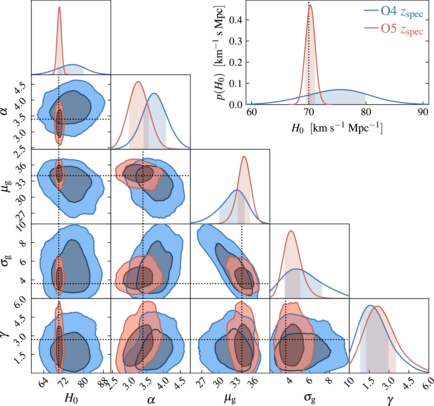