


Abstract
We present the probabilistic stellar mass function (pSMF) of galaxies in the DESI Bright Galaxy Survey (BGS), observed during the One-percent Survey. The One-percent Survey was one of DESI's survey validation programs conducted from 2021 April to May, before the start of the main survey. It used the same target selection and similar observing strategy as the main survey and successfully observed the spectra and redshifts of 143,017 galaxies in the r < 19.5 magnitude-limited BGS Bright sample and 95,499 galaxies in the fainter surface-brightness- and color-selected BGS Faint sample over z < 0.6. We derive pSMFs from posteriors of stellar mass, M*, inferred from DESI photometry and spectroscopy using the Hahn et al. PRObabilistic Value-Added BGS (PROVABGS) Bayesian spectral energy distribution modeling framework. We use a hierarchical population inference framework that statistically and rigorously propagates the M* uncertainties. Furthermore, we include correction weights that account for the selection effects and incompleteness of the BGS observations. We present the redshift evolution of the pSMF in BGS, as well as the pSMFs of star-forming and quiescent galaxies classified using average specific star formation rates from PROVABGS. Overall, the pSMFs show good agreement with previous stellar mass function measurements in the literature. Our pSMFs showcase the potential and statistical power of BGS, which in its main survey will observe >100 × more galaxies. Moreover, we present the statistical framework for subsequent population statistics measurements using BGS, which will characterize the global galaxy population and scaling relations at low redshifts with unprecedented precision.
Export citation and abstract BibTeX RIS

Original content from this work may be used under the terms of the Creative Commons Attribution 4.0 licence. Any further distribution of this work must maintain attribution to the author(s) and the title of the work, journal citation and DOI.
1. Introduction
The galaxy population can largely be characterized by a small number of scaling relations (see Blanton & Moustakas 2009, for a review). This empirical network of scaling relations has been established through large galaxy surveys at all wavelengths, with major optical spectroscopic campaigns such as the Sloan Digital Sky Survey (SDSS; York et al. 2000), Galaxy and Mass Assembly (GAMA) survey (Driver et al. 2011), PRIsm MUlti-object Survey (PRIMUS; Coil et al. 2011), and many others playing a crucial role. Population statistics also encode important information; for instance, the stellar mass function (SMF) precisely characterizes the overall distribution of the stellar mass (M*) of the galaxy population and its evolution across cosmic history (e.g., Cole et al. 2001; Drory et al. 2004, 2009; Fontana et al. 2004; Bundy et al. 2005; Li & White 2009; Marchesini et al. 2009; Ilbert et al. 2010; Pozzetti et al. 2010; Baldry et al. 2012; Moustakas et al. 2013; Muzzin et al. 2013; Mortlock et al. 2015; Bernardi et al. 2017; Leja et al. 2020; Santini et al. 2021; Driver et al. 2022; Weaver et al. 2023). SMFs also serve as key measurements for calibrating galaxy formation models (see Somerville & Davé 2015, and references therein) and can be used to connect the physics of galaxy formation to the hierarchical assembly of structure in the Universe (e.g., Conroy & Wechsler 2009; Guo et al. 2010; Cattaneo et al. 2011; Leauthaud et al. 2012; Reddick et al. 2013; Wang et al. 2013; Rodríguez-Puebla et al. 2017; Girelli et al. 2020).
The relationship between the stellar masses and star formation rates (SFRs) of galaxies reveal a bimodality in the galaxy population with star-forming galaxies lying on a tightly correlated "star-forming sequence" (SFS; Daddi et al. 2007; Noeske et al. 2007; Salim et al. 2007; Elbaz et al. 2011; Speagle et al. 2014; Whitaker et al. 2014; Hahn et al. 2019; Leja et al. 2022; Popesso et al. 2023). The SFS evolves with redshift, with the SFR of galaxies at fixed mass steadily increasing from z = 0 up to at least z ∼ 4. This is also accompanied by a change in the fraction of quiescent galaxies caused by the quenching of star formation in some galaxies (e.g., Ilbert et al. 2013; Muzzin et al. 2013; Santini et al. 2022). Additional scaling relations invoking quantities such as metallicity (e.g., Tremonti et al. 2004; Mannucci et al. 2010), atomic and molecular gas mass (see reviews in Tacconi et al. 2020; Saintonge & Catinella 2022), and galaxy size (e.g., Franx et al. 2008; van der Wel et al. 2014) have also been firmly established. These scaling relations and associated population statistics, along with careful measurements of their scatter and redshift evolution, are powerful tools to shed further light on galaxy formation and evolution.
For one, they have the potential to reveal new trends among galaxies undetected by previous observations and open new discovery space. They can also be used to test galaxy formation models spanning empirical models (e.g., UniverseMachine; Behroozi et al. 2019), semianalytic models (e.g., Benson 2012; Henriques et al. 2015; Somerville & Davé 2015), and hydrodynamical simulations (see Somerville & Davé 2015, for a review). Empirical models, for example, have been used to measure the timescale of star formation quenching(Wetzel et al. 2013; Hahn et al. 2017; Tinker et al. 2017; Reeves et al. 2023) or the dust content of galaxies (Hahn et al. 2022; Zuckerman et al. 2021).
Furthermore, galaxy observables and their scaling relations can also be used to infer parameters that dictate the physical processes in semianalytic models (e.g., Henriques et al. 2009, 2015; Lu et al. 2014). Although full parameter exploration is currently computationally prohibitive for hydrodynamical simulations, they have been extensively compared to observations (e.g., Genel et al. 2014; Davé et al. 2017; Trayford et al. 2017; Dickey et al. 2021; Donnari et al. 2021). Soon, machine-learning techniques for accelerating and emulating simulations will enable us to go beyond such comparisons and broadly explore parameter space and galaxy formation models (e.g., Jamieson et al. 2023; Villaescusa-Navarro et al. 2023). While many different approaches are available for expanding our understanding of galaxies, they all require statistically powerful galaxy samples with well-controlled systematics and well-understood selection functions.
One survey that will provide galaxy samples with unprecedented statistical power is the Dark Energy Spectroscopic Instrument (DESI; Levi et al. 2013; DESI Collaboration et al. 2016a, 2016b; Abareshi et al. 2022). Over its 5 yr operation, DESI will observe galaxy spectra using the 4 m Mayall telescope at Kitt Peak National Observatory with a focal plane filled with 5000 robotically actuated fibers that direct the light to 10 optical spectrographs (Schubnell et al. 2016; Miller et al. 2023; Silber et al. 2023). It will observe ∼40 million galaxy spectra over 360 nm < λ < 980 nm with spectral resolution of 2000 < λ/Δλ < 5500 over ∼14,000 deg2, a third of the sky. In addition, DESI galaxies will also have photometry from the Legacy Imaging Surveys Data Release 9 (LS; Dey et al. 2019; D. J. Schlegel et al., in preparation). The LS is a combination of three public projects (Dark Energy Camera Legacy Survey, Beijing-Arizona Sky Survey (Zou et al. 2017), and Mayall z-band Legacy Survey) that jointly imaged the DESI footprint in three optical bands (g, r, and z). DESI began observing its main survey on 2021 May 14.
As part of its core observations, DESI is conducting the Bright Galaxy Survey (BGS; Hahn et al. 2023b). BGS spans the same 14,000 deg2 footprint and will include low-redshift z < 0.6 galaxies that can be observed during bright time, when the night sky is ∼2.5 × brighter than nominal dark conditions. BGS will provide two galaxy samples: the BGS Bright sample, an r < 19.5 magnitude-limited sample of ∼10 million galaxies, and the BGS Faint sample, a fainter 19.5 < r < 20.175 sample of ∼5 million galaxies selected using a surface brightness and color. The selection and completeness of the BGS samples are characterized in detail in Hahn et al. (2023b; see also Myers et al. 2023). Compared to the seminal SDSS main galaxy survey, BGS will provide a galaxy sample 2 mag deeper, with over twice the sky footprint and double the median redshift z ∼ 0.2. It will observe a broader range of galaxies than previous surveys and provide an opportunity to measure galaxy population statistics with unprecedented precision.
BGS will also be accompanied by a value-added catalog: the PRObabilistic Value-Added BGS (PROVABGS; Hahn et al. 2023a; Kwon et al. 2023). For every BGS galaxy, PROVABGS will provide physical properties such as stellar mass (M*), average SFR ( ), stellar metallicity (Z*), stellar age (tage), and dust content. These galaxy properties will be derived from state-of-the-art spectral energy distribution (SED) modeling of both DESI photometry and spectroscopy in a full Bayesian inference framework. The SED model is designed to minimize model mis-specification by using highly flexible nonparametric star formation history (SFH) and metallicity history (ZH), as well as a flexible dust attenuation model. Furthermore, the properties will be inferred using a fully Bayesian inference framework and will thus provide statistically rigorous estimates of uncertainties and degeneracies among the properties. Ultimately, PROVABGS will provide consistently measured galaxy properties that will enable analyses to take full advantage of the statistical power of BGS with new techniques and approaches.
A key application for PROVABGS will be measuring population statistics using a statistically rigorous methodology that correctly propagates the uncertainties in galaxy property measurements. Current population statistics are by and large derived from simply binning best-fit point estimates of galaxy properties. Malz & Hogg (2022) demonstrated, in the context of inferring redshift distributions from individual photometric redshift measurements, that using point estimates is statistically incorrect and can lead to biased redshift distributions. Similarly, the point estimate approach can also lead to biased population statistics.
Instead, we can estimate population statistics from combining individual PROVABGS posteriors of galaxy properties using population inference in a hierarchical Bayesian framework (e.g., Hogg et al. 2010; Foreman-Mackey et al. 2014; Baronchelli et al. 2020). This approach correctly propagates the uncertainties in the galaxy properties from the individual posteriors of galaxies. As a result, they significantly improve the accuracy of population statistics measurements, account for Eddington bias, and will enable more accurate measurements of key galaxy scaling relations. In this work, we present the first such population statistics measurement for BGS: the probabilistic SMF (pSMF).
In particular, we present the pSMF of BGS galaxies observed during the DESI One-percent Survey, a survey validation (SV) program conducted before the main survey operations. We also present the statistical methodology for the population inference, as well as our methods for accounting for observational systematics and incompleteness. We begin in Section 2 with an overview of the BGS galaxies observed during the DESI One-percent Survey. Then, in Section 3, we briefly summarize the PROVABGS SED modeling framework used to infer the physical properties of the BGS galaxies. Afterward, we present the pSMF inferred from the BGS observations in Section 4. We summarize and discuss our results in Section 5. Throughout this work, we assume AB magnitudes (Oke 1974) and a flat ΛCDM cosmology described by the final Planck results (Planck Collaboration et al. 2014): Ωm = 0.307, Ωb = 0.0483, H0 = 67.8 km s−1 Mpc−1, As = 2.19 × 10⁻⁹, ns = 0.9635.
2. The DESI Bright Galaxy Survey: One-percent Survey
DESI began its 5 yr of operations on 2021 May 14 (D. Kirkby et al. 2023, in preparation; Schlafly et al. 2023). Before its start, DESI conducted the SV campaign to verify that the survey will meets its scientific and performance requirements. The SV campaign was divided into two main programs: the first, SV1, characterized the survey's performance under different observing conditions and was used to optimize sample selection. The second, the One-percent Survey (or SV3), observed a data set that can be used for representative clustering measurements and to deliver a "truth" sample with high completeness over an area at least 1% of the expected main survey footprint. We refer readers to DESI Collaboration et al. (2024) and DESI Collaboration et al. (2023) for details on the DESI SV programs. For details on how DESI targets are selected, we refer readers to Cooper et al. (2023), Raichoor et al. (2023), Zhou et al. (2023), and Chaussidon et al. (2023). 30 In this work, we focus on BGS galaxies observed during the One-percent Survey.
The One-percent Survey was observed on 38 nights from 2021 April to the end of 2021 May. During this time, DESI observed 288 bright time exposures that cover 214 BGS "tiles," planned DESI pointings. The tiles were arranged so that a set of 11 overlapping tiles has their centers arranged around a 0.12 deg circle, forming a "rosette" completeness pattern. In total, the One-percent Survey observed 20 rosettes covering 180 deg2 spanning the northern Galactic cap (see Figure 1 in Hahn et al. 2023b).
All BGS spectra observed during the One-percent Survey are reduced using the "fuji" version of the DESI spectroscopic data reduction pipeline (Guy et al. 2023). First, spectra are extracted from the spectrograph CCDs using the spectroperfectionism algorithm of Bolton & Schlegel (2010). Then, fiber-to-fiber variations are corrected by flat-fielding, and a sky model, empirically derived from sky fibers, is subtracted from each spectrum. Afterward, the fluxes in the spectra are calibrated using stellar model fits to standard stars. The final processed spectra are then derived by co-adding the calibrated spectra across exposures of the same tile. In total, DESI observed spectra of 155,022 BGS Bright and 109,418 BGS Faint targets during the One-percent Survey.
For each spectrum, redshift is measured using Redrock 31 (S. Bailey et al. in preparation; Brodzeller et al. 2023), a redshift fitting algorithm that uses χ2 minimization computed from a linear combination of principal component analysis (PCA) basis spectral templates in three template classes ("stellar," "galaxy," and "quasar"). Redrock also provides measures of redshift uncertainty, ZERR, and redshift confidence, Δχ2, which corresponds to the difference between the χ2 values of the best-fit model and the next best-fit model. We restrict our sample to galaxy targets with reliable redshift measurements, as defined in Hahn et al. (2023b) and DESI Collaboration et al. (2024): we only keep targets with spectra classified as galaxy spectra by Redrock, no Redrock warning flags, Δχ2 > 40, and Redrock redshift uncertainty ZERR < 0.0005(1 + z). We also exclude any targets observed using malfunctioning fiber positioners. Lastly, we impose a redshift range of 0 < z < 0.6. After these cuts, our One-percent Survey BGS sample includes 143,074 BGS Bright galaxies and 96,771 BGS Faint galaxies.
3. PROVABGS SED Modeling
For each BGS galaxy, we derive its M* and other physical properties, such as  , mass-weighted metallicity (ZMW), and mass-weighted stellar age (tage,MW), from DESI photometry and spectroscopy using the PROVABGS SED modeling framework (Hahn et al. 2023a). PROVABGS models galaxy SEDs using stellar population synthesis with a nonparametric SFH with a starburst, a nonparametric ZH that evolves with time, and a flexible dust attenuation prescription. The nonparameteric SFH and ZH prescriptions are derived from SFHs and ZHs of simulated galaxies in the Illustris hydrodynamic simulation (Genel et al. 2014; Vogelsberger et al. 2014; Nelson et al. 2015) and provide compact and flexible representations of SFHs and ZHs. For the stellar population synthesis, PROVABGS uses the Flexible Stellar Population Synthesis (FSPS; Conroy et al. 2009, 2010) model with MIST isochrones (Paxton et al. 2011, 2013, 2015; Choi et al. 2016; Dotter 2016), Chabrier (2003) initial mass function (IMF), and a combination of MILES (Sánchez-Blázquez et al. 2006) and BaSeL (Lejeune et al. 1997, 1998; Westera et al. 2002) spectral libraries. The PROVABGS SED model excludes emission lines by masking the wavelength ranges of emission lines. For dust, PROVABGS uses the two-component Charlot & Fall (2000) attenuation model with birth cloud and diffuse dust components and does not include reradiated dust emission.
Furthermore, PROVABGS provides a Bayesian inference framework that infers full posterior probability distributions of the SED model parameter: p(θ ∣ X photo, X spec), where X photo represents the photometry and X spec represents the spectroscopy. In total, θ has 13 parameters: M*, six parameters specifying the SFH (β1, β2, β3, β4, fburst, tburst), two parameters specifying ZH (γ1, γ2), three parameters specifying dust attenuation (τBC, τISM, ndust), and a nuisance parameter for the fiber aperture effect. Posteriors provide statistically rigorous estimates of uncertainties and capture the degerancies among galaxy properties. Furthermore, they are essential for hierarchical population inference as we later demonstrate.
In practice, accurately estimating a 13-dimensional posterior requires a large number (≳100,000) of SED model evaluations, which requires prohibitive computational resources—roughly 10 CPU hours per galaxy. To address this challenge, PROVABGS samples the posterior using the Karamanis & Beutler (2020) ensemble slice Markov Chain Monte Carlo (MCMC) sampling with the zeus Python package 32 (Karamanis et al. 2021). PROVABGS further accelerates the inference by using neural emulators for the SED models. The emulators are accurate to subpercent level and >100 × faster than the original SED model based on FSPS (Kwon et al. 2023). With zeus and neural emulation, deriving a posterior takes ∼5 minutes per galaxy with PROVABGS. Moreover, Hahn et al. (2023a) used forward-modeled synthetic BGS observations to demonstrate that PROVABGS can accurately infer M* over the full expected M* range of BGS.
In Figure 1, we demonstrate the PROVABGS SED modeling framework for a randomly selected BGS Bright galaxy with z = 0.2768 (target ID: 39627769595825146). In the top panels, we present the posteriors of galaxy properties, M*,  , ZMW, and tage, MW, inferred from DESI photometry and spectroscopy. We mark the 40th, 68th, and 86th percentiles of the posterior with the contours. The posteriors illustrate that we can precisely measure the properties of BGS galaxies from DESI photometry and spectroscopy. Furthermore, with the full posterior, we accurately estimate the uncertainties on the galaxy properties and the degeneracies among them (e.g., M* and
  ). In the bottom panels, we compare the PROVABGS SED model prediction using the best-fit parameter values (black) to DESI observations (blue). The bottom left panel compares the optical g-, r-, and z-band photometry, while the right panel compares the spectra. For reference, we also include the observed spectra with coarser wavelength binning (azure). The comparison shows good agreement between the best-fit model and the observations.
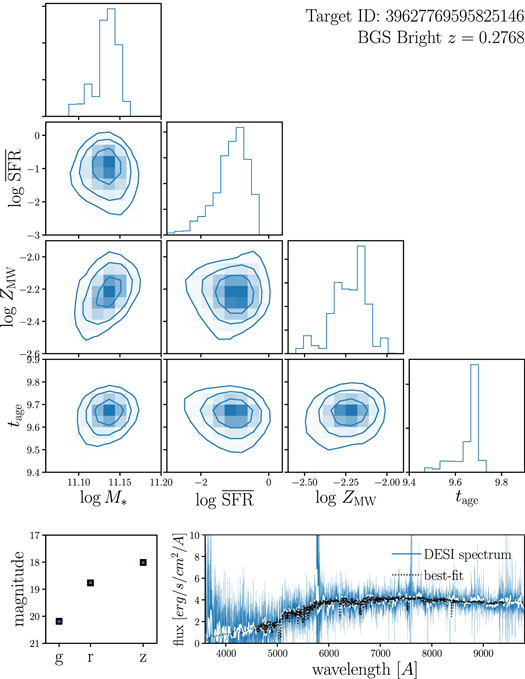
Figure 1. Top panels: posteriors of galaxy properties, M*,  , ZMW, and tage, MW, for a randomly selected BGS Bright galaxy with z = 0.2768 (target ID: 39627769595825146) inferred using the PROVABGS SED modeling framework from DESI photometry and spectroscopy. The contours mark the 40th, 68th, and 86th percentiles of the posterior. With the PROVABGS posteriors, we accurately estimate the galaxy properties, their uncertainties, and any degeneracies among them. Bottom panels: comparison of the best-fit PROVABGS SED model prediction (black) to observations (blue). We compare the g-, r-, and z-band photometry in the left panel and spectra in the right panel. We include the observed spectra with coarser binning for clarity (azure). We use PROVABGS to infer the posterior of galaxy properties for every BGS galaxy in the DESI One-percent Survey.
Download figure:
Standard image High-resolution imageWe derive a PROVABGS posterior (e.g., Figure 1) for every galaxy in the DESI One-percent Survey. In Figure 2, we present the best-fit M* measurements as a function of z for the BGS galaxies in the DESI One-percent Survey. We mark the galaxies in the BGS Bright sample in blue and the ones in the BGS Faint sample in orange.
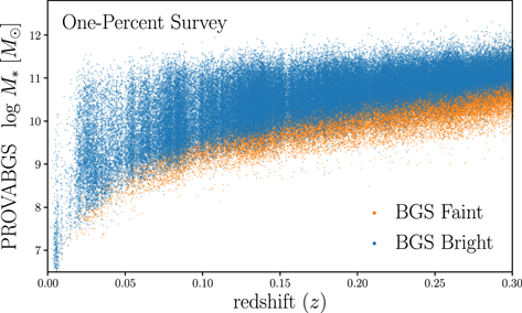
Figure 2. M* as a function of z of BGS Bright (blue) and Faint (orange) galaxies in the DESI One-percent Survey. For M*, we use the best-fit values derived using PROVABGS. BGS Bright is a magnitude-limited sample to r < 19.5, while BGS Faint includes fainter galaxies 19.5 < r < 20.175 selected using surface brightness (rfiber) and color (Hahn et al. 2023b). We note that significant variation in the distribution at low redshift is from large-scale structure. In total, we infer the posteriors of 143,017 BGS Bright and 95,499 BGS Faint galaxies across z < 0.6 in the DESI One-percent Survey.
Download figure:
Standard image High-resolution image4. Results
From the posteriors of galaxy properties inferred using PROVABGS (Section 3), we derive the marginalized 1D posterior of M*, p(M* ∣ X i ), from observed spectrophotometry X i of galaxy i. Using these posteriors, we can estimate the pSMF of BGS galaxies using population inference in a hierarchical Bayesian framework (e.g., Hogg et al. 2010; Foreman-Mackey et al. 2014; Baronchelli et al. 2020). In other words, we can infer p(ϕ ∣ { X i }), the probability distribution of ϕ given the BGS observations, { X i }. ϕ is the set of population hyperparameters that describe the pSMF, Φ(M*; ϕ). This approach is statistically rigorous and enables us to correctly propagate the uncertainties in our M* measurements to the pSMF.
In this work, we estimate the pSMF using a Gaussian mixture model (GMM; Press et al. 1992; McLachlan & Peel 2000; Blanton et al. 2003), which provides a highly flexible description of the M* distribution:
Here k is the number of Gaussian components, and ϕj is the mean and standard deviation of the jth Gaussian component of the GMM. Previous works have used parametric functions (e.g., the Schechter function) to describe the pSMF (e.g., Leja et al. 2020). We opt for GMMs in order to produce a nonparametric measurement of the pSMF that relaxes any assumptions on the functional form of the SMF. In a subsequent work (F. Speranza et al. 2024, in preparation), we will present the BGS pSMF measured using a parametric model with continuous redshift evolution.
To infer p(ϕ ∣ { X i }), we follow the same approach described in Hahn et al. (2023a):


We can estimate the integral using Si Monte Carlo samples from the individual posteriors p(θi ∣ X i ):
Here p(ϕ) and p(θi,j ) are the priors on the population hyperparameters and the SED model parameters. We use uniform distributions, p(ϕ) = 1 and p(θi,j ) = 1, for both priors in this work.
Since the sample of BGS galaxies is not volume limited and complete as a function of M*, we must account for selection effects and incompleteness when estimating the pSMF. We derive stellar mass completeness limits,  , in Appendix C. We also include weights derived from
  , the maximum redshift that galaxy i could have and still be included in the BGS samples. We derive
  for each galaxy by redshifting the SED predicted by the best-fit (maximum likelihood) parameters and determining the maximum z that the galaxy could be placed before it falls out of the survey selection. We use the best-fit parameters, rather than, e.g., samples drawn from the posteriors. However, this does not have a significant effect because BGS spans a relatively narrow redshift range and BGS galaxies are primarily selected using r-band magnitudes. The r-band bandpass lies at the center of DESI spectral wavelength range, so the SED models used to calculate
  would be well constrained by the observed spectrum. We then derive the comoving volume,
  , out to
  , and we include a factor of
  in the galaxy weight wi
.
in the galaxy weight wi
.
Next, we include correction weights for spectroscopic incompleteness driven by fiber assignment and redshift failures. The incompleteness from fiber assignment is due to the fact that DESI is not able to assign fibers to all galaxies included in the BGS target selection. Furthermore, there is significant variation in the assignment probability owing to the clustering of galaxies. Meanwhile, incompleteness from redshift failure is caused by the fact that we do not successfully measure the redshift for every spectrum. The redshift failure rate depends significantly on the surface brightnesses of the galaxies and the signal-to-noise ratio of the spectra. We describe how we derive the incompleteness correction weights for fiber assignment and redshift failures, wi,FA and wi,ZF, in Appendix A. Each BGS galaxy is assigned a weight of  .
.
We modify Equation (4) to include galaxy weights, wi :
The weights are included in the exponent, so, for example, a galaxy with wi = 2 would have the same contribution to p(ϕ ∣ { X i }) as two galaxies with wi = 1.
In practice, we do not derive the full posterior p(ϕ ∣ {
X
i
}). Instead, we derive the maximum a posteriori (MAP) hyperparameter ϕMAP that maximizes p(ϕ ∣ {
X
i
}) or  . We expand,
Since the first two terms are constant, we derive ϕMAP by maximizing
using the Adam optimizer (Kingma & Ba 2017). We derive ϕMAP for BGS galaxies in redshift bins of width Δz = 0.04, starting from z = 0.01, in order to examine the redshift evolution of the SMF within BGS.
4.1. The Probabilistic Stellar Mass Function
We present the pSMF of BGS galaxies in the One-percent Survey in Figure 3 (black line) at 0.01 < z < 0.05. In the left panel, we also present the pSMFs of the BGS Bright (blue) and Faint (orange) galaxies separately. BGS Bright galaxies are selected using an r < 19.5 magnitude limit. As a result, the BGS Bright sample is M* complete above  (black dotted–dashed). We derive
  in Appendix C and mark the pSMF above the completeness limit in solid and below the limit in dashed. Meanwhile, the BGS Faint sample is selected using a surface brightness and color selection. It includes fainter galaxies, 19.5 < r < 20.175, with overall lower M* than BGS Bright. We plot the pSMFs down to the minimum number density that can be measured for our 0.01 < z < 0.05 volume (Gehrels 1986). The shaded regions represent the uncertainties of the pSMF, which we derive using a standard jackknife technique (Appendix B). The jackknife uncertainties conservatively estimate the combined uncertainties from the population inference, as well as cosmic variance (Norberg et al. 2009).

Figure 3. The pSMF of BGS galaxies in the One-percent Survey at 0.01 < z < 0.05 (black line). In the left panel, we present the pSMFs of BGS Bright (blue) and Faint (orange) galaxies, separately. We also include the SMF measured using the standard point estimate approach (black dotted), which underestimates the SMF at the low- and high-mass ends. We represent uncertainties on the pSMF, estimated using a standard jackknife technique, with the shaded regions (Appendix B). The solid line represents the pSMF above the completeness limit  (Appendix C). In the right panel, we include SMF measurements from previous spectroscopic surveys for comparison: SDSS Moustakas et al. (2013), Bernardi et al. (2017), and GAMA (Driver et al. 2022). Overall, the pSMFs of BGS are in good agreement with SMF measurements from previous surveys.
Download figure:
Standard image High-resolution imageWe also include the SMF estimated using the standard point estimate approach (black dotted), derived using the maximum likelihood M* point estimates with the same galaxy weights, wi . At intermediate M* range, 109 M⊙ < M* < 1010.5 M⊙, we find good agreement with the pSMF. However, the standard approach significantly underestimates the SMF outside this M* range. These discrepancies are due to the fact that point estimates of M* ignore the uncertainties in the inferred M*. The impact is significant at the most massive end of the SMF with fewer galaxies. It is also significant at the least massive end, where the observations have lower signal-to-noise ratio, so the individual M* posteriors are broader. The discrepancies are present in all other redshift bins and underscore the importance of correctly propagating the M* uncertainties.
In the right panel, we compare the BGS pSMF to SMF measurements from previous spectroscopic surveys: SDSS (black circle and square; Moustakas et al. 2013; Bernardi et al. 2017) and GAMA (black triangle Driver et al. 2022). We note that there is significant variance in SMF measurements in the literature, especially at the high-M* end. This is partly due to the different modeling methodologies used to derive M*, which can contribute >0.1 dex discrepancies (Pacifici et al. 2023). Furthermore, there are also discrepancies due to photometric corrections applied to SDSS photometry, assumptions on the stellar populations, and dust (Bernardi et al. 2017). We also do not account for differences in the IMF and cosmology. In a subsequent work, we will present a detailed comparison of BGS M* measurements using different methods.
Incompleteness and systematics may also contribute to any discrepancies between our pSMF and other SMF measurements. For our pSMF, we account for spectroscopic incompleteness from fiber assignment and redshift failures (Appendix A). If uncorrected, redshift failures can lead to underestimates of the number of quiescent galaxies without emission lines, which have lower rates of successfully measuring redshifts. We correct for this incompleteness by modeling a galaxy's redshift success rate as a function of its surface brightness, spectral signal-to-noise ratio, color, and a proxy for emission lines. However, there may be additional dependencies not included in our modeling. Additional systematics may also impact the pSMF: for example, our galaxy samples are optically selected and not mass selected using near-IR photometry and may have color-dependent mass incompleteness. Nevertheless, we find overall good agreement with previous SMF measurements, especially in the intermediate M* range where we precisely infer the pSMF.
In Figure 4, we present the redshift evolution of the BGS Bright pSMF over 0.01 < z < 0.17 spanning 2.2 Gyr. The shaded region represents the jackknife uncertainties for the pSMF. The solid line represents the pSMF above  , while the dashed lines represent the pSMF below the limit. We only include four redshift bins with width Δz = 0.04, since
  for z > 0.17 (Table 2). The pSMFs in Figure 4 do not reveal a significant redshift dependence given their uncertainties. We note that the large uncertainties for the 0.01 < z < 0.05 pSMF are driven by large-scale structure at R.A. ∼ 195 deg, decl. ∼ 28 deg, and z ∼ 0.0244. The main BGS survey will observe >100 × more BGS galaxies than the One-percent Survey with comparable signal-to-noise ratio,
33
and it will enable pSMF measurements with unprecedented precision.
for z > 0.17 (Table 2). The pSMFs in Figure 4 do not reveal a significant redshift dependence given their uncertainties. We note that the large uncertainties for the 0.01 < z < 0.05 pSMF are driven by large-scale structure at R.A. ∼ 195 deg, decl. ∼ 28 deg, and z ∼ 0.0244. The main BGS survey will observe >100 × more BGS galaxies than the One-percent Survey with comparable signal-to-noise ratio,
33
and it will enable pSMF measurements with unprecedented precision.
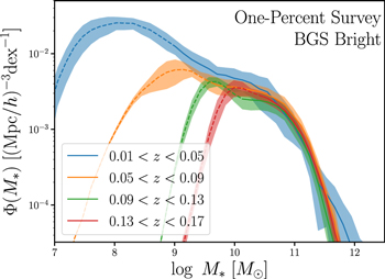
Figure 4. The BGS Bright pSMF over the redshift range 0.01 < z < 0.17 spanning 2.2 Gyr, in bins of Δz = 0.04. The shaded regions represent the uncertainties on the pSMF, estimated using a standard jackknife technique. The solid lines represent the pSMF above the completeness limit  , while the dashed lines represent the pSMF below the limit. We find no significant redshift evolution of the pSMFs over this range. The main BGS survey will observe >100 × more galaxies than the One-precent Survey and will characterize the pSMF redshift evolution even more precisely.
Download figure:
Standard image High-resolution image4.2. Star-forming and Quiescent Galaxies in BGS
In addition to the pSMF of the full galaxy population, we can also examine the pSMF of the star-forming and quiescent subpopulations using  , the average SFR over the past 1 Gyr, inferred with PROVABGS. In Figure 5, we present the distribution of M* versus average specific SFR,
  , for BGS Bright (blue) and Faint (orange) galaxies at z < 0.2. The M*−sSFR distribution of the BGS galaxies reveals a clear bimodality, with star-forming galaxies lying on the SFS and quiescent galaxies lying ≳1 dex below the sequence. Figure 5 also confirms that BGS Faint galaxies have overall lower M* than BGS Bright galaxies and are primarily star-forming galaxies. This is due to the fact that the (z − W1) − 1.2(g − r) + 1.2 color used to select BGS Faint galaxies is a proxy for Hα and Hβ emission lines.

Figure 5. The  distribution of BGS galaxies at z < 0.2. sSFR is derived using
  , the average SFR over the past 1 Gyr, inferred using PROVABGS. The
  distribution is bimodal, with star-forming galaxies lying on the SFS. We classify galaxies with
  as star-forming galaxies and galaxies with
  as quiescent.
Download figure:
Standard image High-resolution imageTo further examine the star-forming and quiescent galaxy populations, we classify BGS Bright galaxies as star-forming or quiescent using an  cut. We determine this cut empirically based roughly on the
  of the "green valley" between the SFS and the quiescent mode. We opt for an
  cut rather than more sophisticated methods in the literature (e.g., Donnari et al. 2019; Hahn et al. 2019) for simplicity. In Figure 6, we present the pSMF of star-forming and quiescent BGS Bright galaxies at 0.01 < z < 0.17 in bins of Δz = 0.04. The shaded regions represent the jackknife uncertainties for the pSMF. The solid lines represent the pSMFs above the completeness limit, while the dashed lines represent the pSMFs below the limit. Overall, the pSMFs show little evolution over these M* and redshift ranges except for a possible decline at the massive end of the star-forming pSMF.
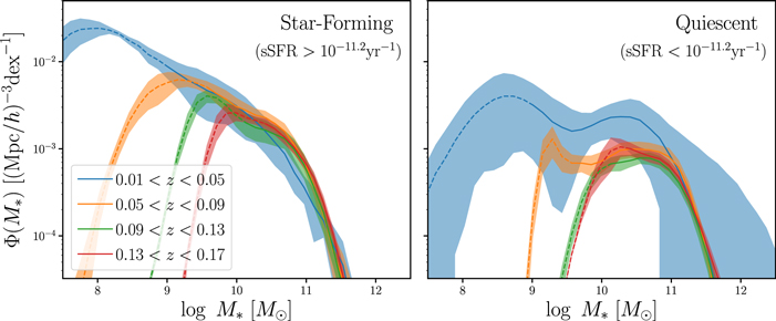
Figure 6. The pSMF of star-forming (left) and quiescent (right) BGS Bright galaxies over 0.01 < z < 0.17 in bins of Δz = 0.04. Star-forming and quiescent galaxies are classified using an empirically determined sSFR = 10−11.2 yr−1 cut. We represent the uncertainties for the pSMF in the shaded regions and the pSMFs above/below the M* completeness limits in solid/dashed lines. We find little overall evolution of the pSMFs over the redshift range investigated here.
Download figure:
Standard image High-resolution imageNext, we present the fraction of quiescent galaxies in BGS Bright as a function of M* over 0.01 < z < 0.17 in Figure 7. The quiescent fraction is derived by taking the ratio of the pSMFs of quiescent galaxies over all galaxies and measured for each Δz = 0.04 bin. The shaded region represents the uncertainties derived from propagating the jackknife uncertainties of the pSMFs. We focus on the quiescent fraction of BGS Bright galaxies above the M* completeness limit:  . At each redshift bin, the quiescent fraction increases with M* to ∼1 at M* ∼ 1011.5
M⊙. We find no significant redshift evolution of quiescent fraction across 0.01 < z < 0.17. Although the significant statistical uncertainties obfuscate a clear trend, the quiescent fraction evolution is in good qualitative agreement with previous works (e.g., Baldry et al. 2006; Iovino et al. 2010; Peng et al. 2010; Hahn et al. 2015). Upcoming observations from the DESI main survey will increase the number of BGS galaxies by >100 × and enable precise comparisons of the quiescent fraction measurements.
. At each redshift bin, the quiescent fraction increases with M* to ∼1 at M* ∼ 1011.5
M⊙. We find no significant redshift evolution of quiescent fraction across 0.01 < z < 0.17. Although the significant statistical uncertainties obfuscate a clear trend, the quiescent fraction evolution is in good qualitative agreement with previous works (e.g., Baldry et al. 2006; Iovino et al. 2010; Peng et al. 2010; Hahn et al. 2015). Upcoming observations from the DESI main survey will increase the number of BGS galaxies by >100 × and enable precise comparisons of the quiescent fraction measurements.
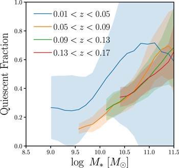
Figure 7. The quiescent fraction of BGS Bright galaxies over 0.01 < z < 0.17 in bins of Δz = 0.04. We present the uncertainties in the shaded region and only include the quiescent fraction above the M* completeness limit. The quiescent fractions increase with M* at all redshifts. We find no significant redshift evolution of the quiescent fraction over our redshift range.
Download figure:
Standard image High-resolution image5. Summary and Discussion
Over its 5 yr operation, starting on 2021 May, the DESI BGS will observe the spectra of ∼15 million galaxies out to z < 0.6 over 14,000 deg2. BGS will produce two main galaxy samples: an r < 19.5 magnitude-limited BGS Bright sample and a fainter 19.5 < r < 20.175 surface-brightness- and color-selected BGS Faint sample. Compared to the SDSS main galaxy survey, the BGS galaxy samples will be over 2 mag deeper, cover more than twice the footprint, and have double the median redshift z ∼ 0.2. They will include diverse galaxy subpopulations that have the potential to reveal new trends among galaxies that were previously undetectable and open new discovery space.
In addition, each galaxy in BGS will have measurements of its detailed physical properties (e.g., M*, SFR, Z*, tage) from PROVABGS. These properties will be inferred from DESI spectrophotometry using state-of-the-art SED modeling in a fully Bayesian inference framework. PROVABGS will provide statistically rigorous estimates of uncertainties and degeneracies among the properties. With these measurements alongside its statistical power, BGS will provide a powerful galaxy sample with which to measure scaling relations and population statistics that will characterize the global galaxy population and test galaxy formation models with unprecedented precision.
In this work, we showcase the potential of BGS by presenting the pSMF using ∼250,000 BGS galaxies observed solely during one of DESI's SV programs. The pSMFs are derived using a hierarchical population inference framework that statistically and rigorously propagates uncertainties on M* and provide improved estimates of the SMF at the lowest and highest M* regimes. We also describe how we account for selection effects and incompleteness in the BGS observations (Appendix A). Overall, we find good agreement between our pSMF and previous SMF measurements in the literature. We also examine the pSMF of the star-forming and quiescent galaxy population classified using a simple  cut and find qualitative agreement with previous works.
This work is first of a series of papers that will present population statistics for BGS galaxies using PROVABGS. For the pSMF in this work, we used a flexible GMM to provide a nonparametric measurement of the SMF. In a subsequent work (F. Speranza et al. 2024, in preparation), we will present the pSMF of BGS measured using a parametric model with continuous redshift evolution. In another work, we will present in-depth comparison of M* measured using different methodologies and assumptions. We will also explore the color dependence of the fiber aperture effect and its impact on inferred galaxy properties in M. Ramos et al. (2024, in preparation). Lastly, the hierarchical population inference framework presented in this work can be extended to population statistics beyond the SMF. We will extend the framework to the SFR−M* distribution and present the probabilistic SFR−M* distribution and quiescent fraction in future work.
All of the pSMFs presented in this work are measured from BGS galaxies observed from 2021 April to May during the DESI One-percent Survey. Since then, DESI has already completed nearly 2 yr of observations. As of writing (2023 May), DESI has observed over 22 million galaxy spectra in total and over 10 million BGS galaxy spectra. With 3 out of the 5 yr of operation remaining, BGS has completed ∼60% of its observations and is ahead of schedule. BGS will also be further extended by additional low-redshift dwarf galaxies observed with the DESI low-z secondary program (Darragh-Ford et al. 2023). DESI observations will be publicly released periodically, starting with the Early Data Release (EDR) later this year. The EDR will include observations from the One-percent Survey used in this work. An accompanying PROVABGS catalog will be released with each data release. All of the pSMF measurements and data used to generate the figures presented in this work are publicly available at doi:10.5281/zenodo.8018936.
Acknowledgments
It's a pleasure to thank Alex I. Malz and Peter Melchior for helpful discussions. We also thank Rita Tojeiro and Rebecca Canning for their detailed review and feedback on an earlier version of this work. This work was supported by the AI Accelerator program of the Schmidt Futures Foundation.
This material is based on work supported by the U.S. Department of Energy (DOE), Office of Science, Office of High Energy Physics, under contract No. DE-AC02-05CH11231, and by the National Energy Research Scientific Computing Center, a DOE Office of Science User Facility, under the same contract. Additional support for DESI was provided by the U.S. National Science Foundation (NSF), Division of Astronomical Sciences under contract No. AST-0950945 to the NSF's National Optical-Infrared Astronomy Research Laboratory; the Science and Technologies Facilities Council of the United Kingdom; the Gordon and Betty Moore Foundation; the Heising-Simons Foundation; the French Alternative Energies and Atomic Energy Commission (CEA); the National Council of Science and Technology of Mexico (CONACYT); the Ministry of Science and Innovation of Spain (MICINN); and the DESI Member Institutions: https://www.desi.lbl.gov/collaborating-institutions.
The DESI Legacy Imaging Surveys consist of three individual and complementary projects: the Dark Energy Camera Legacy Survey (DECaLS), the Beijing-Arizona Sky Survey (BASS), and the Mayall z-band Legacy Survey (MzLS). DECaLS, BASS, and MzLS together include data obtained, respectively, at the Blanco telescope, Cerro Tololo Inter-American Observatory, NSF's NOIRLab; the Bok telescope, Steward Observatory, University of Arizona; and the Mayall telescope, Kitt Peak National Observatory, NOIRLab. NOIRLab is operated by the Association of Universities for Research in Astronomy (AURA) under a cooperative agreement with the National Science Foundation. Pipeline processing and analyses of the data were supported by NOIRLab and the Lawrence Berkeley National Laboratory. Legacy Surveys also use data products from the Near-Earth Object Wide-field Infrared Survey Explorer (NEOWISE), a project of the Jet Propulsion Laboratory/California Institute of Technology, funded by the National Aeronautics and Space Administration. Legacy Surveys was supported by the Director, Office of Science, Office of High Energy Physics of the U.S. Department of Energy; the National Energy Research Scientific Computing Center, a DOE Office of Science User Facility; the U.S. National Science Foundation, Division of Astronomical Sciences; the National Astronomical Observatories of China; the Chinese Academy of Sciences; and the Chinese National Natural Science Foundation. LBNL is managed by the Regents of the University of California under contract to the U.S. Department of Energy. The complete acknowledgments can be found at https://www.legacysurvey.org/.
Any opinions, findings, and conclusions or recommendations expressed in this material are those of the author(s) and do not necessarily reflect the views of the U.S. National Science Foundation, the U.S. Department of Energy, or any of the listed funding agencies.
The authors are honored to be permitted to conduct scientific research on Iolkam Du'ag (Kitt Peak), a mountain with particular significance to the Tohono O'odham Nation.
Appendix A: Spectroscopic Completeness
Spectroscopic galaxy surveys, such as BGS, do not successfully measure the redshift for all of the galaxies they target. As a result, this spectroscopic incompleteness must be accounted for when measuring galaxy population statistics such as the SMF. In this appendix, we present how we estimate the spectroscopic incompleteness for BGS and derive the weights we use to correct for its impact on the SMF.
For BGS, spectroscopic incompleteness is primarily driven by fiber assignment and redshift failures. DESI uses 10 fiber-fed spectrographs with 5000 fibers but targets more galaxies than available fibers. For instance, the BGS Bright and Faint samples have ∼860 and 530 targets deg−2, respectively. In addition, of the 5000, a minimum of 400 "sky" fibers are dedicated to measuring the sky background for accurate sky subtraction, and an additional 100 fibers are assigned to standard stars for flux calibration (Guy et al. 2023).
Furthermore, each fiber is controlled by a robotic fiber positioner on the focal plane. These positioners can rotate on two arms and be positioned within a circular patrol region of radius 1 48 (DESI Collaboration et al. 2016a; Schubnell et al. 2016; Abareshi et al. 2022; Silber et al. 2023). Although the patrol regions of adjacent positioners slightly overlap, the geometry of the positioners causes higher incompleteness in regions with high target density (Smith et al. 2019). To mitigate the incompleteness from the fiber assignment, BGS will observe its footprint with four passes. With this strategy, BGS achieves ∼80% fiber assignment completeness (Hahn et al. 2023b).
To estimate fiber assignment completeness, we run the fiber assignment algorithm (Raichoor et al. 2023) on BGS targets 128 separate times. For each BGS galaxy, i, we count the total number of times out of 128 fiber assigned realizations that the galaxy is assigned a fiber: Ni,FA. Then, to correct for the fiber assignment incompleteness, we assign correction weights
to each BGS galaxy.
Although we measure a spectrum for each galaxy assigned a fiber, we do not measure reliable redshifts for all spectra that meet the criteria specified in Section 2. This redshift measurement failure significantly contributes to spectroscopic incompleteness. For BGS, redshift failure of an observed galaxy spectrum depends mainly on fiber magnitude and a statistic, TSNR2. Fiber magnitude is the predicted flux of the BGS object within a 1 5-diameter fiber; we use r-band fiber magnitude, rfiber. TSNR2 roughly corresponds to the signal-to-noise ratio of the spectrum and is the statistic used to calibrate the effective exposure times in DESI observations (Guy et al. 2023). Redshift failure also depends on the galaxy type and whether the galaxy has emission lines in its spectrum.
In Figure 8, we present the redshift success rate of BGS Bright galaxies as a function of rfiber and TSNR2. In each hexbin, the color map represents the mean z-success rate. We include all hexbins with more than two galaxies. Overall, the z-success rate depends significantly on rfiber: galaxies with fainter rfiber have lower z-success rates. However, the rfiber dependence itself varies in bins of TSNR2. We mark the edges of the bins in black dashed: logTSNR2 = 2.0, 2.5, 3.0, 3.5, 3.85. Within each of the TSNR2 bins, the rfiber dependence of the z-success rate does not vary significantly. In Figure 9, we present the z-success rate of BGS Bright galaxies as a function of rfiber for each of the six TSNR2 bins. We mark the range of TSNR2 in the lower left corner of each panel. The error bars represent the Poisson uncertainties of the z-success rate.
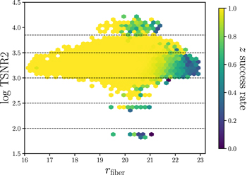
Figure 8. Redsift success rate of BGS Bright galaxies as a function of rfiber and TSNR2. TSNR2 is a statistic that quantifies the signal-to-noise ratio of the observed spectrum. The color map represents the mean redshift success rate in each hexbin. We mark the TSNR2 bins (black dashed) that we use to separately fit the redshift success rate as a function of rfiber using Equation (A3). In each TSNR2 bin, redshift success decreases as rfiber increases.
Download figure:
Standard image High-resolution image
Figure 9. Redshift success rates of BGS Bright galaxies as a function of rfiber in six TSNR2 bins. The error bars represent the Poisson uncertainties. In each panel, we include the best-fit analytic (Equation (A3)) approximation of the redshift success rate (dashed) derived from χ2 minimization. We use this analytic approximation to calculate the galaxy weights to correct for spectroscopic incompleteness caused by failures to accurately measure redshifts from observed spectra.
Download figure:
Standard image High-resolution imageTo correct for the effect of redshift failures, we include an additional correction weight for each BGS galaxy:
Here fz−sucess is the z-success rate as a function of rfiber, TSNR2, g − r color, and grzW1 − color of the galaxy; grzW1 − color = (z − W1) − 1.2(g − r) + 1.2 is the color proxy for Hα and Hβ emission lines, also used in the BGS Faint selection. Galaxies with fz−sucess = 1 (100% z-success) will have wi,ZF = 1.0, while galaxies with fz−success = 0.1 (10% z-success) will have wi,ZF = 10.
To estimate fz−sucess, we fit the functional form
separately for the TSNR2 bins: 101.5−102.0, 101.5−102.5, 102.5−103.0, 103.0−103.5, 103.5−103.85, 103.85−105. For all TSNR2 bins other than 103.0−103.5, c0 and c1 are constants, and we do not include a g − r or grzW1 − color dependence since we do not detect a significant dependence of fz−success on galaxy color. However, for the TSNR2 bin 103.5−103.85, we include the g − r and grzW1 − color dependence in c0 = c0,0 + c0,1(g − r) + c0,2(grzW1 − color) and c1 = c1,0 + c1,1(g − r) + c1,2(grzW1 − color). All of the best-fit coefficients are derived from χ2 minimization. We estimate fz−success independently for BGS Bright galaxies, BGS Faint galaxies with (z − W1) − 1.2(g − r) + 1.2 ≥ 0, and BGS Faint galaxies with (z − W1) − 1.2(g − r) + 1.2 < 0. For BGS Faint, we do not detect a significant g − r and grzW1 − color dependence, so we only include the dependence on TSNR2 and rfiber.
In Figure 9, we present the best-fit fz−success(rfiber) for each of the TSNR2 bins in dashed. In the 103.0 < TNSR2 < 103.5 range, we illustrate the g − r dependence by comparing the best fits for the galaxies in two subsamples split by g − r < 1. We list the best-fit values in bins of TSNR2 for each of the samples in Table 1. Despite the efforts above to correct for spectroscopic incompleteness, we caution that our correction is likely incomplete, as properties beyond TSNR2, rfiber, g − r, and grzW1 − color may impact our z-success rate.
Table 1. Best-fit Coefficients of Equation (A3), which Describes the z-success Rate as a Function of rfiber for Different TSNR2 Bins for BGS Bright and Faint Samples
| TSNR2 Range | c0 | c1 |
|---|---|---|
| BGS Bright | ||
| 101.5–102 | 0.443 | 19.7 |
| 102–102.5 | 0.668 | 21.3 |
| 102.5–103 | c0,0 = 0.946 | c1,0 = 23.0 |
| c0,1 = 0.979 | c1,1 = − 3.28 | |
| c0,2 = − 0.134 | c1,2 = 0.299 | |
| c0,3 = − 3.59 | c1,2 = 11.6 | |
| 103–103.5 | 0.822 | 22.4 |
| 103.5–103.85 | 0.698 | 23.3 |
| 103.85–105 | 0.465 | 21.8 |
| BGS Faint | ||
| (z − W1) − 1.2(g − r) + 1.2 ≥ 0 | ||
| 101.5–102.5 | 1.67 | 21.1 |
| 102.5–103 | 1.65 | 21.8 |
| 103–103.1 | 1.49 | 22.1 |
| 103.1–103.2 | 1.32 | 22.3 |
| 103.2–103.3 | 1.33 | 22.4 |
| 103.3–103.5 | 0.907 | 23.1 |
| 103.5–103.85 | 1.03 | 23.0 |
| 103.85–105 | 0.924 | 21.6 |
| BGS Faint | ||
| (z − W1) − 1.2(g − r) + 1.2 < 0 | ||
| 102.5–103 | 1.48 | 20.9 |
| 103–103.1 | 2.40 | 21.2 |
| 103.1–103.2 | 1.30 | 21.8 |
| 103.2–103.3 | 1.27 | 22.0 |
| 103.3–103.5 | 1.83 | 21.6 |
| 103.5–103.85 | 0.798 | 22.9 |
| 103.85–105 | 1.29 | 20.6 |
Download table as: ASCIITypeset image
In future works with the BGS main survey, our samples will have >100 × more galaxies. This will enable us to significantly improve our modeling of redshift failures and better correct for spectroscopic incompleteness. We will also explore using emission-line measurements from FastSpecFit (Moustakas 2023, J. Moustakas 2024, in preparation) to further improve our modeling. Furthermore, we will also include corrections for additional incompleteness and systematics, such as corrections for imaging systematics using multivariate regression (e.g., Ross et al. 2017) or machine-learning methods (Rezaie et al. 2020) currently being developed for the DESI cosmology analyses.
Appendix B: Uncertainties on the SMF
We estimate the uncertainties of the pSMF from cosmic variance using the standard jackknife technique. We split the BGS sample into subsamples and then estimate uncertainties using the subsample-to-subsample variations:
Njack is the number of jackknife subsamples, and Φk represents the SMF estimated from the BGS galaxies excluding the jackknife subsample k. In this work, we split the BGS sample into 12 jackknife fields based on the angular positions of galaxies. We present the jackknife fields in Figure 10 with distinct colors.
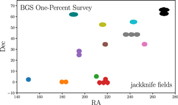
Figure 10. The R.A. and decl. of the 12 jackknife fields of the BGS One-percent Survey used to estimate the uncertainties on the SMF from cosmic variance. We mark each field with a distinct color.
Download figure:
Standard image High-resolution imageAppendix C: Stellar Mass Completeness
In this appendix, we describe how we derive  , the M* limit above which our BGS Bright sample is complete. Although there are various methods for estimating
  in the literature, e.g., based on estimating the mass-to-light ratio (Pozzetti et al. 2010; Moustakas et al. 2013), we adopt an approach that takes advantage of the fact that BGS Bright is a magnitude-limited sample, where galaxy subsamples at lower redshifts are complete down to lower M* than than those at higher redshifts.
To derive  in redshift bins of width Δz = 0.04, we first split the galaxy sample into narrower bins of Δz/2. For each narrower redshift bin, iΔz/2 < z < (i + 1)Δz/2, we take the best-fit PROVABGS SEDs for all of the galaxies in the bin and artificially redshift them to
  . Then, at
  , the galaxies would have fluxes of
Here dL
(z) represents the luminosity distance at redshift z. Afterward, we calculate the r-band magnitudes,  , for
, for  and impose the
  magnitude limit of the BGS Bright sample. We then compare the M* distribution of all the galaxies in iΔz/2 < z < (i + 1)Δz/2 to the galaxies in (i + 1)Δz/2 < z < (i + 2)Δz/2 with
  . For instance, we present the M* distributions of all BGS Bright galaxies in 0.01 < z < 0.03 (blue) and the BGS Bright galaxies in 0.01 < z < 0.03 with
  (orange) in Figure 11.

Figure 11. The M* distribution of BGS Bright galaxies with 0.01 < z < 0.03 (blue) and the M* distribution of the same set of galaxies that would remain in the BGS Bright magnitude limit if they were redshifted to  . We set the stellar mass completeness limit,
  , for 0.01 < z < 0.05 to the M* where more than 10% of galaxies are excluded in the latter distribution. For each Δz bin, we repeat this procedure to derive
  values.
Download figure:
Standard image High-resolution imageSince galaxies become fainter when they are placed at higher redshifts, i.e.,  , the
, the  sample has fewer low-M* galaxies. We determine the M* at which more than 10% of galaxies are excluded in the
  sample (black dashed) and set this limit as
  for the redshift bins: 0.01 < z < 0.05. Our procedure for deriving
  takes advantage of the fact that galaxy samples at lower redshifts are complete down to lower M* than at higher redshifts. We repeat this procedure for all the Δz = 0.04 redshift bins that we use to measure the SMF. In Table 2, we list
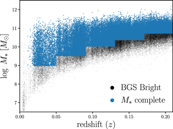
  values for each of the redshift bins. Furthermore, we present the M* and redshift relation of BGS Bright galaxies (black) and the stellar mass complete sample (blue) in Figure 12.
Figure 12.
M* and redshift relation of BGS Bright galaxies in the One-percent Survey (black) and the galaxies within the stellar mass completeness limit ( blue).
  is derived in redshift bins of width Δz = 0.04. The lowest redshift bin (0.01 < z < 0.05) is complete down to M* < 109
M⊙.
is derived in redshift bins of width Δz = 0.04. The lowest redshift bin (0.01 < z < 0.05) is complete down to M* < 109
M⊙.
Download figure:
Standard image High-resolution image
Table 2. Stellar Mass Completeness Limit,  for Redshift Bins of Width Δz = 0.04
| z Range |

|
|---|---|
| 0.01–0.05 | 8.975 |
| 0.05–0.09 | 9.500 |
| 0.09–0.13 | 10.20 |
| 0.13–0.17 | 10.38 |
| 0.17–0.21 | 10.72 |
Download table as: ASCIITypeset image
Footnotes
- 30
- 31
- 32
- 33
The One-percent Survey was observed using exposure times 1.2 × longer than the main survey.