


Abstract
The Galactic global magnetic field is thought to play a vital role in shaping Galactic structures such as spiral arms and giant molecular clouds. However, our knowledge of magnetic field structures in the Galactic plane at different distances is limited, as measurements used to map the magnetic field are the integrated effect along the line of sight. In this study, we present the first ever tomographic imaging of magnetic field structures in a Galactic spiral arm. Using optical stellar polarimetry over a  field of view, we probe the Sagittarius spiral arm. Combining these data with stellar distances from the Gaia mission, we can isolate the contributions of five individual clouds along the line of sight by analyzing the polarimetry data as a function of distance. The observed clouds include a foreground cloud (d < 200 pc) and four clouds in the Sagittarius arm at 1.23, 1.47, 1.63, and 2.23 kpc. The column densities of these clouds range from 0.5 to 2.8 × 1021 cm−2. The magnetic fields associated with each cloud show smooth spatial distributions within their observed regions on scales smaller than 10 pc and display distinct orientations. The position angles projected on the plane of the sky, measured from the Galactic north to the east, for the clouds in increasing order of distance are 135°, 46°, 58°, 150°, and 40°, with uncertainties of a few degrees. Notably, these position angles deviate significantly from the direction parallel to the Galactic plane.
Export citation and abstract BibTeX RIS

Original content from this work may be used under the terms of the Creative Commons Attribution 4.0 licence. Any further distribution of this work must maintain attribution to the author(s) and the title of the work, journal citation and DOI.
1. Introduction
Magnetic fields significantly contribute to the hydrostatic balance in the interstellar medium (ISM; Boulares & Cox 1990; Ferrière 2001; Cox 2005; Han 2017). Magnetic pressure and magnetic tension caused by magnetic fields are both nonuniform forces acting perpendicularly to the magnetic field lines. Therefore, magnetic fields are believed to introduce anisotropy in the gas motion and consequently have a significant impact on structure formation and evolution in the ISM, ranging from galaxy formation to the formation of filamentary molecular clouds within a single star-forming region (Heiles & Crutcher 2005; Boulanger et al. 2018). Indeed, magnetic field lines are expected to be influenced by the motion of the ISM, leading to their dragging or bending (e.g., Doi et al. 2021a; Tahani 2022; Tahani et al. 2023). As a result, the interstellar magnetic field structure is expected to be inscribed with a history of the deformation of the ISM (Gómez et al. 2018). In other words, by revealing the structure of the interstellar magnetic field, we can elucidate the formation history of the ISM structure (e.g., Tahani 2022; Tahani et al. 2022a, 2022b). Mapping the distribution of magnetic fields from the spatial scale of individual molecular clouds to Galactic scales (10 pc–1 kpc scales) may therefore provide critical information for understanding the role of, for example, the Galactic spiral arms in the formation of giant molecular clouds and the subsequent star formation inside them (e.g., Han 2017; Zucker et al. 2018; Stephens et al. 2022).
The structure of magnetic fields can be studied by observing polarized radiation arriving from astronomical objects. Asymmetric dust particles irradiated by incoming radiation fields align their rotation axes parallel to the ambient magnetic field direction (radiative alignment torques; Lazarian & Hoang 2007). This process causes polarized light from both extincted background stars and thermal dust emission from the grains themselves (Stein 1966; Hildebrand 1988). Thus, the plane-of-sky (POS) component of the magnetic field (BPOS), associated with dust particles that are primarily in the cold neutral ISM (≲100 K; McKee 1995), can be observed with both stellar optical/near-infrared polarimetry and submillimeter polarimetry (Lazarian 2007). However, one of the limitations of these observational techniques, particularly of polarimetry of optically thin dust emission, is that they can only obtain the average value of the superimposed magnetic field components along the line of sight (LOS). Especially for regions close to the Galactic plane, multiple clouds can be found along the LOS and that can complicate the inferred BPOS from optically thin dust.
In recent years, Gaia data have provided accurate distances to stars (Gaia Collaboration et al. 2016, 2023; Bailer-Jones et al. 2021) and interstellar extinction values for these stars (Andrae et al. 2023; Babusiaux et al. 2023). By combining these pieces of information with stellar polarimetry data, it becomes possible to reveal the 3D distribution of the ISM and its associated magnetic field up to distances of a few kiloparsecs (e.g., Panopoulou et al. 2019; Doi et al. 2021b; Pelgrims et al. 2023).
The Galactic magnetic field is expected to be nearly parallel to the Galactic disk (i.e., BZ ≃ 0) and correlated with the spiral arms (Beck 2013, 2015; Beck & Wielebinski 2013; Haverkorn 2015; Han 2017). Polarimetry of dust emission shows a magnetic field distribution that is generally parallel to the Galactic plane (Novak et al. 2003; Li et al. 2006; Bierman et al. 2011; Bennett et al. 2013; Planck Collaboration et al. 2016). On the other hand, the magnetic field of the neutral ISM traced by stellar polarimetry is not always parallel to the Galactic plane (Heiles 2000; Clemens et al. 2020; Choudhury et al. 2022), and a variation of the position angle (PA) along the LOS has been observed (Pavel 2014; Zenko et al. 2020). We need more detailed observational information to reveal the magnetic field structure along the LOS (e.g., Jaffe 2019).
The Sagittarius arm is one of the four major spiral arms of the Galaxy and is observed at −14° ≲ l ≲ +50° of the Galactic plane (Vallée 2022). This structure is the closest major spiral arm in the inner Galactic plane and harbors massive-star-forming regions such as M8, M16, M17, and M20 (Kuhn et al. 2021). The l ≳ +20° region is heavily obscured by the Aquila Rift in the foreground (approximately 200–500 pc along the LOS), but there are no noticeable foreground clouds at l ≲ +20°. In addition, the arm is almost entirely in the POS in the smaller Galactic longitude range (l ≲ +20°), allowing us to estimate the large-scale magnetic field structure that follows the Galactic arm structure with good approximation from the observed PA of BPOS. Furthermore, target stars are more abundant in the inner Galactic plane than in the outer Galactic plane, making it a good target for obtaining the 3D magnetic field from stellar polarimetry.
To reveal the magnetic field structure along the LOS in the Sagittarius arm by a stellar polarimetric survey, this paper, as a first step, will demonstrate that we can identify multiple ISM clouds and their associated local magnetic field structure along the LOS, including the amplitude of the direction dispersion of the turbulent magnetic fields.
This paper is organized as follows. In Section 2, we describe the selection of the observation area within the Sagittarius arm, the observations, and the data reduction procedure. Section 3 provides a detailed analysis of the distance dependence of the observed magnetic field PAs along the LOS. It discusses the identification of clouds through statistical analysis of the polarimetry data, as well as the magnetic field characteristics specific to each cloud. Section 4 discusses the relationship between the observed distance dependence and the magnetic field traced by submillimeter polarimetry observed by the Planck satellite, which is integrated along the LOS, as well as the amplitude of the turbulent magnetic field in each cloud. In Section 5, we summarize the results.
2. Observations and Data Reduction
2.1. Target Selection
We selected the Sagittarius arm, the nearest major spiral arm in the inner Galactic plane with abundant observable stars in optical polarimetry, as our first target to create a tomographic image of the magnetic field in a spiral arm. We observed a target field within +10° < l < +20° to avoid the Aquila Rift and to have a good sky position from the Higashi-Hiroshima Observatory (see Section 2.2).
To define the target region, in addition to the above constraints, we imposed the following conditions, referring to the Gaia Data Release 2 (DR2; Gaia Collaboration et al. 2018) catalog, which was the latest Gaia release when the observation was being planned:
- 1.A sufficient number of stars (≳100) with Gaia distances are distributed across all distances up to ∼3 kpc.
- 2.The interstellar extinction increases gradually with distance along the LOS, rather than experiencing concentrated increases at specific distances.
These conditions impose a continuous sampling of the magnetic field across the Sagittarius arm along the LOS. Consequently, we selected a  field centered at l = +14
 15, b = −147.
2.2. Observations
We obtained linear polarimetry in the Cousins R band (RC band: λ = 0.65 μm) using the Hiroshima Optical and Near-infrared Camera (HONIR; Akitaya et al. 2014) on the 1.5 m Kanata Telescope, Higashi-Hiroshima Observatory, on 2021 August 5. The optics of the HONIR instrument consists of a rotating half-wave plate, a focal mask of five equally spaced slits with a 50% opening ratio, and a Wollaston prism that splits the incident light into two orthogonally polarized images next to each other on the detector focal plane (see Section 5 of Akitaya et al. 2014). As a result, five pairs of images with orthogonal polarizations are exposed across the entire surface of the detector. To cover the  detector field of view (FOV) with multiple exposures, we made 3 × 3 spatial dithers with a 31
 2 step in the east–west direction and a 200 step in the north–south direction.
To measure the polarization parameters q ≡ Q/I and u ≡ U/I of each star, we acquired photometry with four PAs of the half-wave plate at 0°, 45°, 225, and 675 (Kawabata et al. 1999). As a result, we obtained a total of 36 exposures, with each exposure lasting 75 s.
We covered the target field using two adjacent FOVs centered at l = +1411, b = −141 and l = +1418, b = −153. The combined FOV size was  as shown in Figure 1.

Figure 1. Observed stellar polarization pseudovectors (white line segments). The data of 105 stars with errors on PA δPA ≤ 10° are shown, out of 184 stars with significant polarization detection and accurate distance estimation. A reference scale of P is shown in the lower left corner of the figure. The background is from the Second Generation Digitized Sky Survey red image (McLean et al. 2000). The orange line segments are magnetic field PAs obtained from Planck data at 353 GHz (Planck Collaboration et al. 2020a; resolution set to  ). The Planck line segments only show the orientation of the magnetic field, estimated by rotating the polarization PA by 90°, and their length is not related to the Planck-measured polarization degree.
Download figure:
Standard image High-resolution imageWe measured stellar intensities by aperture photometry using SExtractor (Bertin & Arnouts 1996). The typical size of the point-spread function is ∼18, and we fixed the aperture diameter to 65 (24 pixels).
2.3. Calibration
We calibrated the instrumental polarization by observing the unpolarized standard star G191-B2B on 2021 July 27. The measured instrumental polarization, an offset vector to the origin in the q–u parameter space, is qinst = 0.01% ± 0.02% and uinst = −0.04% ± 0.02%, which are negligible for our measurements. The stability of the instrumental polarization, measured over a period of 10 months including the observational period, is consistently better than 0.1%, and is thus considered negligible for our measurements. The variation of the instrumental polarization across the detector is better than 0.1% and can also be considered negligible (Akitaya et al. 2014).
We calibrated the polarization PA by observing the strongly polarized standard stars BD+64 106, BD+59 389, and HD 204827 (Schmidt et al. 1992) on 2021 July 27 and August 30. The achieved calibration accuracy is better than 04 and the stability during the observational period was estimated to be better than 03.
We calibrated the polarization efficiency of the instrument by observing an artificially polarized star through a wire-grid polarizer inserted before the half-wave plate. The measured efficiency is 99.1% ± 0.01%, by which we scaled the observed polarization fractions.
We converted the measured normalized Stokes parameters, q and u, defined in equatorial coordinates, into Galactic coordinates, qGal and uGal. This transformation allowed us to align the polarization measurements with the Galactic coordinate system for further analysis and interpretation. The details of the coordinate conversion process are described in Appendix A.
2.4. Gaia Identification and Selection
We referred to the Gaia Data Release 3 (DR3; Gaia Collaboration et al. 2023) catalog and cross-matched the observed stars with detections of polarization within a search radius of 1''. We referred to a Gaia-based catalog by Bailer-Jones et al. (2021) for the distance of each star. Among their distance estimations, we adopted "geometric" distances, including distance estimates for all our observed stars.
We limited our search by applying the conditions of a renormalized unit weight error ≤1.4 and a parallax_over_error ≥3 in the Gaia DR3 catalog, and a stellar distance uncertainty (a 68% confidence interval) ≤20%. In addition, we selected data with an estimated error δ P ≤ 0.3% for the fractional polarization, which was typically achieved by stars with RC ≤ 15.5 mag. Following this procedure, we identified 184 stars within the observed field. In investigating interstellar extinction in the observed region, we referred to 259 stars meeting the criteria of distance uncertainty ≤20% and AG values available in the DR3 catalog. There were 130 stars found in both data sets. We analyzed all available data for both polarization and extinction, regardless of their availability in the other data set. We summarize the identified stars in Table 6 in Appendix B.
3. Results
3.1. Spatial and Distance Distribution of Polarimetry Data
Figure 1 shows the spatial distribution of the observed polarization pseudovectors (white segments), indicating the PAs and polarization fractions (P). The derivation of these values from the observed q and u values is detailed in Appendices A and B. Of the 184 stars employed in the following analyses, 105 stars with a polarization PA uncertainty δPA ≤ 10° are plotted in the figure. The distribution of BPOS traced by stellar polarimetry appears to be a perfect mix of various PAs in space. The histogram of PAs shown in Figure 2 shows a bimodal distribution centered around 30° and 140°. PA = 90°, which is the direction parallel to the Galactic plane, corresponds to the minimum of the distribution. Thus the observed BPOS is not parallel to but predominantly tilted from the Galactic plane. The PAs and their distribution do not show particular variations or trends with sky coordinates (Figure 1).

Figure 2. Histogram of PAs. The bin width is set to 20°. We show 105 stars with δPA ≤ 10°, the same as in Figure 1. The two black arrows indicate the PA of Planck's magnetic field inside the observed region (see Figure 1; the spatial resolution is set to  ). The vertical dotted line represents the PA for the Galactic plane (PA = 90°).
Download figure:
Standard image High-resolution imageFigures 1 and 2 also show Planck's observed magnetic field PA for the same region (orange segments). In the following, we refer to the polarimetry data observed by the Planck satellite at 353 GHz (data release 3; Planck Collaboration et al. 2020a), as provided by IRSA (Planck Team 2020), with a resolution set to  .
.
Given that the Stokes parameters in the Planck data products are provided in the HEALPix convention rather than the IAU convention, we estimate the polarization PA of the data using the following equation:

We estimate the PA of the magnetic field by rotating the polarization PA observed by Planck by 90°. We will use the term "Planck's observed magnetic field" or "the Planck magnetic field" for simplicity. Similar to our stellar polarimetry data, the Planck magnetic field shows PAs deviating from 90° (1400, 711, 1210, and 660 from north to south in Figure 1). However, the angle offset from 90° is generally larger for the stellar polarimetry magnetic field orientations.
The distance dependence of the optical polarimetry data is shown in Figure 3. Specifically, we show how PA and P vary as a function of the Gaia stellar distances estimated by Bailer-Jones et al. (2021). Note that PA is mostly nonparallel to the Galactic plane, as shown in Figure 2.
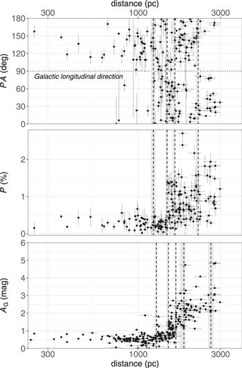
Figure 3. Distance dependence of polarimetry data (PA and P; our observed 184 values) and AG (the Gaia DR3 cataloged 259 values). An observed PA of 90° indicates that the magnetic field is parallel to the Galactic plane. The vertical dashed lines indicate the breakpoints of the polarimetry data and AG estimated by the breakpoint analysis. Shaded areas correspond to 68% confidence intervals of the estimation. See text and Doi et al. (2021b) for the details of the breakpoint analysis.
Download figure:
Standard image High-resolution imageFigure 3 also shows interstellar extinction (AG) values taken from the Gaia DR3 catalog. We find an apparent increase of about 2 mag in AG at distances beyond ∼1.2 kpc. It further becomes AG ≥ 2.5 mag beyond ∼2 kpc. We can attribute this increase in interstellar extinction at distances of about 1.2–2 kpc to the dust in the Sagittarius arm. The foreground component of AG < 1 mag can be attributed to the cloud(s) in the outskirts of the Aquila Rift at d < 200 pc (Section 1), and it is likely related to the Local Bubble shell (Lallement et al. 2019; Pelgrims et al. 2020).
3.2. Identification of Four Dust Clouds along the LOS Using Breakpoint Analysis
Doi et al. (2021b) showed that breakpoint analysis, a statistical technique that detects the points at which data values make stepwise changes, can effectively recover the distance dependence of stellar polarimetry data. Based on this breakpoint analysis, Doi et al. (2021b) characterized the distribution of dust clouds as a function of distance along the LOS and the 3D structure of the magnetic field associated with those clouds. The details of the breakpoint analysis are described in Appendix C. We apply the breakpoint analysis to our observed qGal and uGal, assuming a step change at each breakpoint and constant values between them, as was done by Doi et al. (2021b). We identify four breakpoints, as shown in Table 1 (Polarimetry) and by the dashed lines in Figure 3 (top two panels), together with 68% confidence intervals of the estimation.
Table 1. Breakpoints Estimated in qGal, uGal, and AG
| Breakpoints | |||||
|---|---|---|---|---|---|
| (pc) | |||||
| Polarimetry |

|

|

|

| |
| AG |

|

|

|

|

|
Notes. The error values indicate the 68% confidence intervals of the estimation. See text for the breakpoint analysis.
Download table as: ASCIITypeset image
We also perform breakpoint analysis for the AG values similar to that for the polarimetry data. The results are shown in Table 1 (AG) and Figure 3 (the bottom panel). We can find reasonable agreement between the two independent evaluations. In particular, the three breakpoint distances on the near side show good consistency. On the other hand, the AG analysis finds an extra breakpoint at larger distances and these two farther breakpoints are roughly on either side of the polarimetry breakpoint. We note that there are fewer stars with Gaia-estimated AG values than stars with polarimetry data in this distance range (d > 1.6 kpc; the number of stars in each distance range is listed in Table 2). Also, we find a significant step change in PA at 2.2 kpc (Figure 3). As the focus of this paper is on the magnetic field structure inferred from the polarization data, we utilize the breakpoints detected in the polarization data analysis, which are expected to directly trace changes in the magnetic field structure, in the subsequent analyses.
Table 2. Fitted Parameters within Each Distance Range
| Distance Range | No. of Stars | qGal | uGal | AG | ||||
|---|---|---|---|---|---|---|---|---|
| (kpc) | qGal, uGal | AG | σa | p-value b | σa | p-value b | σa | p-value b |
| <1.23 | 45 | 104 | 0.46 | 0.647 | 0.55 | 0.585 | 0.03 | 0.977 |
| 1.23–1.47 | 29 | 42 | 0.37 | 0.708 | 0.14 | 0.889 | 0.67 | 0.503 |
| 1.47–1.63 | 25 | 39 | 0.25 | 0.803 | 0.18 | 0.859 | 0.69 | 0.487 |
| 1.63–2.23 | 61 | 54 | 0.88 | 0.378 | 0.05 | 0.957 | 1.43 | 0.153 |
| >2.23 | 24 | 20 | 0.11 | 0.911 | 0.68 | 0.497 | 1.17 | 0.241 |
Notes.
a Statistical deviation of the maximum likelihood slope value from 0. b Statistical p-value for the null hypothesis that the slope of the distribution is equal to 0.Download table as: ASCIITypeset image
In the breakpoint analysis, as in Doi et al. (2021b), we assume that the values of qGal and uGal are both constant between neighboring breakpoints. To validate this assumption, we perform a linear fitting on each parameter between breakpoints to test if the slope is statistically consistent with a value of 0. We perform the Student t-test for qGal and uGal, and AG as well. The statistical p-values, which are for the null hypothesis that the slope of the distribution is equal to 0, are shown in Table 2. The null hypothesis that the slope of the distribution is equal to 0, i.e., a constant value, cannot be rejected as the p-values are all greater than 5% for the tested cases.
Among the test results, in the two distance ranges under d ≥ 1.63 kpc, where the breakpoint estimate of AG differs from that of the polarimetry data, AG shows smaller p-values. However, the p-values are larger than 15% and are still consistent with the assumption of constant AG values at each distance range defined by the polarimetry. Therefore, these analysis results can be considered as supporting evidence for the validity of the breakpoint analysis of the polarimetry data.
The constancy of the qGal and uGal values within each distance range implies that there is a discrete contribution of polarizing dust sheets at the breakpoints, while there is no significant contribution between breakpoints. In Figure 4, we visually confirm this discrete polarization along the LOS by presenting a cumulative sum plot of the qGal–uGal vectors with increasing distance. In this plot, the sum vector defines a straight line while the PAs of the polarization remain constant if the PAs of the vectors are aligned. This is because the vector sum averages out the random component of each vector. On the other hand, if they are not aligned, a change in the polarization PA turns the direction of the path of the cumulative sum plot.
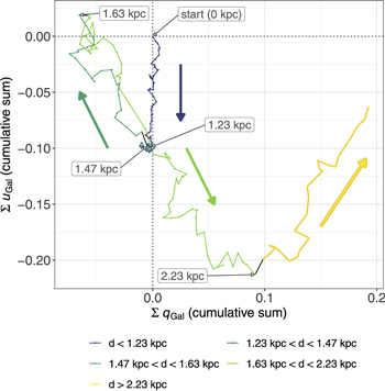
Figure 4. Cumulative sum plot of observed qGal–uGal vectors, which are ordered by distance and shown as colored lines. The qGal–uGal vectors are represented in fractions, with 0.1 corresponding to a polarization of 10%. The labels indicate the stellar distances associated with the polarimetry breakpoints as listed in Table 1. Additionally, the starting point of the sum vector is labeled with "start." The cumulative sum vectors are clearly divided into five sections, consisting of four line segments and a clump between 1.23 and 1.47 kpc. Colored arrows indicate the direction of the cumulative sum vector in each line segment.
Download figure:
Standard image High-resolution imageAs shown in Figure 4, the cumulative sum can be described by the combination of five sections, including four line segments and a clump between 1.23 and 1.47 kpc. The four line segments indicate that the qGal–uGal vectors are well aligned in each distance range. The phase angle of the qGal–uGal vector on the ∑qGal–∑uGal plane corresponds to twice the PA, and therefore, it should be noted that vectors pointing in opposite directions (e.g., the green and light green vectors in the figure) differ by 90° in PA. The clump between 1.23 and 1.47 kpc shows that the length of the qGal–uGal vectors is 0 on average, which indicates that the vectors are aligned in one orientation in this distance range (due to the complete depolarization by the foreground cloud in this case). In summary, Figure 4 shows that the polarization vectors as a whole are well aligned in a specific direction for each of the five distance ranges, with discrete contributions of thin polarizing dust sheets at the breakpoints. Different colors depict the distance range between the breakpoints, which correspond well to each line segment and clump.
The scattered distribution of dust clouds and their discrete contribution to the polarization (Figure 4) is comparable to the finding for the Perseus and (foreground) Taurus molecular clouds (Doi et al. 2021b) and the thin-layer model developed for high Galactic latitude clouds (Pelgrims et al. 2023). This suggests that the thin-layer model is also applicable to LOSs at low Galactic latitudes. Therefore, in the following, we will assume that the discrete dust sheets/clouds at the four breakpoints, in addition to a foreground component before the first breakpoint, generate polarization in each distance range—that is, "foreground," "1.23 kpc cloud," "1.47 kpc cloud," "1.63 kpc cloud," and "2.23 kpc cloud."
Within the distance range where we identify dust clouds along the LOS (d = 1.2–2.2 kpc from the Sun), the vertical offset from the Galactic plane is ∣Z∣ = 32–57 pc. This vertical distance is comparable to or less than the scale height of the Galactic thin disk component (50–70 pc; Nakanishi & Sofue 2006; Kalberla et al. 2007; Yao et al. 2017) and well below that of the disk component of Galactic magnetic field models (100–400 pc; Sun et al. 2008; Jansson & Farrar 2012; Jaffe et al. 2013; Han et al. 2018). Therefore, we are likely observing the Galactic disk component of the magnetic field.
We estimate the 3D distribution of dust clouds in the Galactic disk by applying the breakpoint analysis to the AG values, as described in Appendix D. The color scale in Figure 5 represents the surface density of these dust clouds within a range of ±100 pc from the Galactic plane. The red dashed line in the figure indicates the LOS of the observation. The positions of the four identified dust clouds along the LOS are indicated by their respective distances.
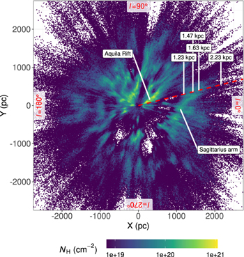
Figure 5. The red dashed line represents the sightline of the observation, while the positions of the four identified dust clouds (indicated by their distances) are shown on the Galactic plane. The coordinates are heliocentric Galactic Cartesian coordinates, with the Sun located at the coordinate origin. The X-axis points toward the Galactic center, the Y-axis points in the direction of Galactic rotation (the Galactic plane at l = 90°), and the Z-axis points toward the Galactic north pole (not depicted in the figure). The color scale represents the surface density of the dust cloud within Z = ±100 pc (see Appendix D for the surface density estimation). The regions of high dust surface density surrounding the 1.23, 1.47, and 1.63 kpc clouds correspond to the Sagittarius spiral arm.
Download figure:
Standard image High-resolution imageThe high dust surface density structure observed around the 1.23, 1.47, and 1.63 kpc clouds in Figure 5 corresponds to the Sagittarius arm. The surface density around the 2.23 kpc cloud appears to be relatively low. However, this does not necessarily imply the absence of dust clouds or the absence of the Sagittarius and Scutum arm structures, as dust clouds located on the far side within the Sagittarius arm may go undetected, being hidden behind dust clouds on the near side of the Sagittarius arm or other foreground clouds.
In summary, our observations identify multiple clouds in the Sagittarius arm and detect polarization at each distance range.
3.3. Magnetic Field Structure of Each Dust Cloud
We show the distribution of polarization pseudovectors and their PAs for each distance range in Figures 6 and 7. As in Figures 1 and 2, we plot only the data points with good PA determination (δPA ≤ 10°), which correspond to 105 objects. The overall distribution of PAs in Figures 1 and 2 appears spatially uncorrelated with a large scatter. However, if we plot the data independently for each distance bin, as shown in Figures 6 and 7, the polarization pseudovectors instead show a well-ordered pattern.

Figure 6. Spatial distribution of the observed PAs for each distance range. Here we plot 105 data with uncertainties δPA ≤ 10°.
Download figure:
Standard image High-resolution image
Figure 7. Histogram of the polarization angles for each distance range. We plot data with uncertainties δPA ≤ 10°. The bin width of the histograms is 20°. The vertical dotted line indicates PA = 90°, which is the PA parallel to the Galactic plane.
Download figure:
Standard image High-resolution imageWe present the mean orientation and angular dispersion of the PAs for each distance range in Table 3, calculated using the circular mean and circular standard deviation. The circular mean and the circular standard deviation (hereafter  ) account for the 180° ambiguity of the polarization pseudovectors. This approach allows for an unbiased estimation of the standard deviation of the PAs, even if the deviation exceeds 50°, and is capable of capturing a wider, though not infinite, range of deviations in the PA measurements compared to the usual arithmetic standard deviation, which saturates at
  (Doi et al. 2020).
19
(Doi et al. 2020).
19
Table 3. Angular Mean and Standard Deviation of PAs within Each Distance Range
| Distance Range | Cloud | Circular Mean | Circular SD 
| ||||
|---|---|---|---|---|---|---|---|
| Equatorial Coordinates | Galactic Coordinates | ||||||
| Observed | Intrinsic | Observed | Intrinsic | Observed | Differential | ||
| (kpc) | (deg) | (deg) | (deg) | (deg) | (deg) | (deg) | |
| <1.23 | foreground |

|
a

|

|
a

|

|
a

|
| 1.23–1.47 | 1.23 kpc |

|

|

|

|

|

|
| 1.47–1.63 | 1.47 kpc |

|

|

|

|

|

|
| 1.63–2.23 | 1.63 kpc |

|

|

|

|

|

|
| >2.23 | 2.23 kpc |

|

|

|

|

|

|
| All |

|
a

|

|
a

|

|
a

| |
Notes. The raw observed values for each distance range are shown in the "Observed" columns. The mean intrinsic PA for each cloud, calculated by subtracting the foreground contributions of all components in front of the respective cloud, is presented in the "Intrinsic" columns. The circular standard deviation values minus the foreground contribution are shown in the "Differential" column. Note that they are biased by the variation caused by the observational error and do not show the intrinsic magnetic field angular variation of each cloud. See text and Doi et al. (2020) for the definitions of the circular mean and the circular standard deviation.
a The "intrinsic" and "differential" values of the foreground cloud and the "all" values are the same as the observed values because there is no foreground component to be subtracted.Download table as: ASCIITypeset image
We utilize all 184 objects selected according to the criteria described in Section 2.4, including those with large δPA, for estimating the circular mean and  . This is in contrast to Figures 1, 2, 6, and 7, which display data from only 105 objects. To estimate the uncertainty of each parameter, we perform 10,000 Monte Carlo simulations. In each simulation, we add Gaussian random errors independently to the relative Stokes parameters q and u based on their respective uncertainties. From the generated samples, we calculate P and PA and obtain the required quantities for the analysis. We show the median value of the 10,000 estimates as the maximum likelihood value and the 15.9% and 84.1% quantiles as the negative and positive errors in Table 3 and in succeeding estimations in this paper.
The angular dispersions ( ) of the observed polarization pseudovectors are found in the "Observed" column in Table 3. Except for the 1.23–1.47 kpc distance range, where the polarization pseudovectors are almost of zero length due to the geometrical depolarization, the angular dispersion for each distance range is significantly smaller than that of the total data, confirming that the polarization pseudovectors of each distance bin are better aligned.
To accurately evaluate the magnetic field structure associated with each cloud, it is important to consider that the observed polarization is a result of integrating all contributions along the optical path to the stars. The relative Stokes parameters qGal and uGal can be approximated as an addition of the contributions from each element along the LOS, particularly in the case of low polarization levels (say, ≪10%; e.g., Patat et al. 2010; Panopoulou et al. 2019; Pelgrims et al. 2023). By subtracting the foreground contribution from the observed polarization in each distance range, we can obtain a more reliable approximation of the intrinsic magnetic field structure associated with each cloud. This allows us to isolate the specific magnetic field characteristics within each cloud, independently of the foreground effects.
The observed qGal and uGal data for the nth distance range on the LOS are the sum of the contributions from all distance ranges from the first to the nth. Similarly, the observed qGal and uGal data for the (n − 1)th distance range are the sum of the contributions from the first to the (n − 1)th distance ranges. Therefore, to obtain the qGal and uGal values of the nth distance range, we can subtract the (n − 1)th data from the nth data, i.e., we can differentiate the observed qGal and uGal values of each distance range.
Figure 8 shows the qGal–uGal data distribution for all distance groups. We also plot the 1σ contours of the qGal–uGal data scatter for each distance range. We can see that the data are discriminated by distance. We estimate the average intrinsic polarization of each interstellar cloud by subtracting the average observed data of the immediately preceding cloud from the average observed data of a particular cloud. The average intrinsic polarization vector is represented by each black line segment in Figure 8. For each data point, similarly, we can obtain a better approximation of the qGal and uGal values of individual clouds by subtracting the average values of qGal and uGal of the immediately preceding cloud, which represents the integration of the contributions of foreground clouds. The subtraction of foreground contributions is thus equivalent to shifting the coordinate origin of the qGal–uGal plane to the average of the qGal and uGal values of the immediately preceding cloud. We will discuss the connection between this shift of origin and an anticorrelation between P and  in Section 4.1.

Figure 8. Distribution of qGal–uGal by distance range. The colored contours are the 1σ contours of the qGal–uGal data scatter for each distance range. The black line segments connect the average qGal–uGal values of individual distance ranges and indicate the intrinsic polarization of each cloud.
Download figure:
Standard image High-resolution imageFigures 9 and 10 depict the distribution of polarization pseudovectors specific to each distance range, obtained by subtracting the mean foreground polarization. Comparing them to the raw observed values plotted in Figures 6 and 7, we observe that the polarization pseudovectors in each distance range exhibit better alignment. This alignment enhancement can be attributed to the subtraction of the mean foreground polarization, which effectively shifts the origin of the qGal–uGal plane to the average foreground value, as discussed earlier. Consequently, this adjustment often elongates the qGal–uGal vectors (resulting in increased P) and aligns them more coherently. The improved alignment of these polarization pseudovectors indicates a well-ordered magnetic field associated with each dust cloud. The spatial scale of the observed region is approximately 5–10 pc, as indicated by the scales shown in Figure 9. This suggests that the spatial structure of the magnetic field associated with each cloud appears smooth at scales smaller than 5–10 pc, with a scale length of the magnetic field structure larger than 10 pc.

Figure 9. Same as Figure 6, but with the polarization pseudovectors of each cloud adjusted by subtracting the average foreground contribution and correcting for their average PA and P values. It is important to note that the individual pseudovectors in the figure are not corrected for the contribution of the foreground component to the variance of PA and P; this correction can only be made statistically. Therefore, the vectors depicted in the figure are corrected only for their average values.
Download figure:
Standard image High-resolution image
Figure 10. Same as Figure 7, but with the PA values of each cloud adjusted by subtracting the average foreground contribution.
Download figure:
Standard image High-resolution imageHowever, it is important to note that in Figure 9, we only subtract the mean foreground polarization, which means that the depicted vectors are corrected for the mean foreground contributions and not their variances. The contribution of the foreground component to the variance of PA and P can only be estimated statistically, and polarization pseudovectors cannot be corrected individually for this contribution.
Additionally, the observed variance of PA, or  , does not arise from a linear sum of contributions from each element along the LOS, as will be discussed in Section 4. Moreover, the observed values of
  are positively biased due to observation errors. Therefore, we compute the variance of qGal–uGal vectors (
 ) specific to individual clouds by removing the foreground cloud's contribution as follows:
where the variance of qGal–uGal for the nth cloud is denoted as  , and the variance of qGal–uGal for the immediately preceding cloud is denoted as
  .
.
Subsequently, this derived variance of qGal–uGal vectors is employed to determine the variance in PA specific to individual clouds. For a more precise evaluation of the variance of PA, we will provide further discussion in Section 4.2.
Table 3 presents the circular mean and circular standard deviation of the polarization PAs for both the raw observed values (listed in the "Observed" columns) and the differential values. The differential values of the circular means are considered intrinsic to the magnetic field associated with each cloud, and we label these estimations as "intrinsic" values in the table.
On the other hand, the differential values of  in Table 3 do not represent the angular dispersions specific to individual clouds, as explained previously. Therefore, in Table 3, we label the differential values of
  as "differential" instead of "intrinsic."
In the following discussions, our primary focus will be on the intrinsic properties of the magnetic field associated with each cloud, unless stated otherwise.
3.4. Polarization Fraction and Polarization Efficiency of Each Dust Cloud
Table 4 shows the polarization fraction (P) for each cloud. To obtain these intrinsic P values, we subtract the average observed qGal and uGal values of the immediately preceding cloud from the average observed qGal and uGal values of the specific cloud, and subsequently convert them into the polarization fraction (P). This estimation can be visualized as the length of the black line segments in Figure 8. The average P values of the raw observed data used for evaluating the intrinsic P values are listed in Appendix E.
Table 4. Polarization Fraction and Polarization Efficiency within Each Distance Range
| Cloud | Polarization Fraction (P) | AG | NH a | Polarization Efficiency |
|---|---|---|---|---|
| (%) | (mag) | (1021 cm−2) | (% mag−1) | |
| Foreground |

|

|

|

|
| 1.23 kpc |

|

|

|

|
| 1.47 kpc |

|

|

|

|
| 1.63 kpc |

|

|

|

|
| 2.23 kpc |

|

|

|

|
| All b |

|

|

|

|
Notes.
a NH = AG · 2.21 × 10²¹/0.789 is assumed (Güver & Özel 2009; Wang & Chen 2019). b Average of all the observed data.Download table as: ASCIITypeset image
To estimate the column density of each cloud, we utilize the Gaia DR3 cataloged interstellar extinction (AG; Andrae et al. 2023). We calculate the average AG within the ranges corresponding to each cloud and subtract the average AG value of the immediately preceding cloud from the average AG value of the specific cloud.
We estimate the column density (NH) of each cloud based on these AG values, assuming AV = AG/0.789 (mag; Wang & Chen 2019) and NH/AV = 2.21 × 10²¹ (H atoms cm−2 mag−1; Güver & Özel 2009). The estimated AG and NH values are presented in Table 4. The average AG and NH values of the raw observed data used for evaluating these intrinsic AG and NH values can be found in Appendix E.
The estimated intrinsic AG of each cloud ranges from 0.17 to 0.98 mag, corresponding to relatively low column densities of NH ≲ 2.76 × 10²¹ (H atoms cm−2). This is because we have selected an observational FOV with relatively low interstellar extinction and with high-accuracy measurements from Gaia's optical trigonometry. In other words, the observed magnetic field is not associated with star-forming regions within dense molecular clouds, but rather with the diffuse gas that likely surrounds the molecular gas in isolated clouds. In fact, no corresponding CO molecular cloud is found in our FOV in catalogs (Rice et al. 2016; Miville-Deschênes et al. 2017), indicating that the gas is primarily atomic. H i surveys (e.g., Kalberla et al. 2005; Kalberla & Haud 2015) do not resolve the clouds due to low spatial and spectral resolutions, so the velocity dispersion of each dust cloud is unknown. Chen et al. (2020) identified dust clouds by referring to Gaia DR2 interstellar extinction data. Their cloud No. 505 at l = 14821, b = −1107 and cloud No. 506 at l = 13370, b = −0212 may correspond to our observed cloud(s) because of their spatial proximity to our FOV (l = 1415, b = −147). The angular distances between the outer edges of their clouds and our FOV are ∼05 (for the spatial extent of the clouds, see their Figures 505 and 506 available online).
20
The distance estimate of cloud No. 505 is 1815.2 ± 42.8 pc and that of cloud No. 506 is 1793.0 ± 42.3 pc. The average distance of our four detected clouds (1.23, 1.47, 1.63, and 2.23 kpc), weighted by their column densities, is estimated to be  pc. This average distance is almost identical to the distances of cloud No. 505 and No. 506. We find more overlapping clouds in the LOS than in the literature, suggesting that we have detected tenuous dust clouds thanks to the distinct change in the magnetic fields' PAs as a function of distance.
We estimate the polarization efficiency (e.g., Whittet 2022) by dividing P by AG, as tabulated in Table 4. The estimated polarization efficiency specific to individual clouds is 0.4% mag−1 for the foreground cloud and 1.0%–1.4% mag−1 for the clouds in the Sagittarius arm. In a similar analysis, Doi et al. (2021b) estimated a polarization efficiency of 1.5% mag−1 for the Taurus and Perseus molecular clouds. Taking into account the difference between the two observations (0.7625 μm for Taurus and Perseus (Goodman et al. 1990) and 0.65 μm for this work) and assuming a wavelength dependence of the fractional polarization of P ∝ λ−1.8 (Mathis 1990), it corresponds to approximately 2.0% mag−1. Therefore, the observed efficiencies in our study are relatively lower than those estimated for the Taurus and Perseus molecular clouds using the same method.
The pitch angle (the angle relative to the direction of the Galactic rotation) of the Sagittarius arm around the observed region is estimated to be ψ ≃ 17° (Reid et al. 2019). Assuming the magnetic field follows the spiral arm structure, the magnetic field in the observation field is inclined to the POS by i = 35° (see Figure 5). In this case, the expected polarization fraction is approximately 0.7 times the maximum value, or 1.4% mag−1, if the maximum value is ∼2.0% mag−1 as observed in the Taurus and Perseus clouds, based on the relation  . That is, the lower polarization efficiency found in the Sagittarius arm compared to that in the Taurus and Perseus molecular clouds may be partly due to the tilted magnetic field orientation to the POS in the Sagittarius arm and the nearly parallel orientation to the POS in Taurus and Perseus (e.g., Jansson & Farrar 2012). The difference in polarization efficiency of clouds in the Sagittarius arm may indicate that the magnetic field structure in the arm has a substantial variation in the in-plane direction of the Galaxy in addition to the direction perpendicular to the Galactic plane. This variation in polarization efficiency may arise from a combination of factors, including differences in the alignment of dust particles and the intricate geometry of the magnetic field.
4. Discussion
4.1. Anticorrelation between PA Dispersion and Polarization Fraction
Planck Collaboration et al. (2020b) reported an anticorrelation between the dispersion of polarization angles and the polarization fraction (also see Fissel et al. 2016). They attributed this anticorrelation to variations in the magnetic field structure along the LOS. Figure 11 illustrates the mean observed polarization fraction (P) and PA dispersion ( ) estimated for each distance range in the optical polarimetry data. These values, presented as the "observed" values of
  and P in Tables 3 and 4, represent measurements of multiple magnetic field components superimposed along the LOS at their respective distances. In other words, Figure 11 showcases the relationship between P and
  associated with different numbers of magnetic field layers along the LOS.
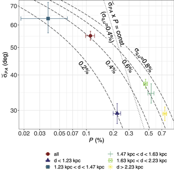
Figure 11. Relationship between the observed values of the polarization fraction (P) and the polarization angle dispersion ( ) in our samples. The dashed lines represent the relationship between the PA dispersion and the P value, based on the marginal distribution of PAs described by Equation (2). These lines are plotted for σq,u
values of 0.8%, 0.6%, 0.4%, and 0.2%, representing different levels of dispersion. The diagonal dotted line shows the approximation of the theoretical P dependence, which corresponds to the
) in our samples. The dashed lines represent the relationship between the PA dispersion and the P value, based on the marginal distribution of PAs described by Equation (2). These lines are plotted for σq,u
values of 0.8%, 0.6%, 0.4%, and 0.2%, representing different levels of dispersion. The diagonal dotted line shows the approximation of the theoretical P dependence, which corresponds to the  correlation pointed out by Planck Collaboration et al. (2020b), in the case of σq,u
= 0.4% (see also Figure 12).
correlation pointed out by Planck Collaboration et al. (2020b), in the case of σq,u
= 0.4% (see also Figure 12).
Download figure:
Standard image High-resolution imageThe data presented in Figure 11 show an anticorrelation, albeit one with a slightly shallower slope compared to the correlation reported by Planck Collaboration et al. (2020b) as  In the following analysis, we will investigate whether this shallower anticorrelation can be attributed to the same correlation reported in Planck Collaboration et al. (2020b).
4.1.1. Theoretical Curve
A geometrical depolarization caused by multiple magnetic field layers along the LOS is equivalent to shifting the coordinate origin of the q–u plane, as discussed in Section 3.3. When the origin of the coordinate system deviates further from the distribution of q and u data, the polarization fraction P increases proportionally. At the same time, the polarization PA dispersion  decreases approximately inversely, particularly when P is sufficiently large. This dependence of
  on P is the same as that of the estimation error of PA derived from the observed qGal and uGal when the standard deviations of qGal and uGal (σq
and σu
) are interpreted as uncertainties in qGal and uGal, respectively, rather than as standard deviations. For isotropic uncertainty distributions where σq
≈ σu
≡ σq,u
, the marginal probability distribution G of PAs can be expressed as follows (Naghizadeh-Khouei & Clarke 1993; Quinn 2012):
on P is the same as that of the estimation error of PA derived from the observed qGal and uGal when the standard deviations of qGal and uGal (σq
and σu
) are interpreted as uncertainties in qGal and uGal, respectively, rather than as standard deviations. For isotropic uncertainty distributions where σq
≈ σu
≡ σq,u
, the marginal probability distribution G of PAs can be expressed as follows (Naghizadeh-Khouei & Clarke 1993; Quinn 2012):
Here, P0 and PA0 represent the average values of P and PA, respectively, and "erf" denotes the Gaussian error function.
We can estimate the angular dispersion  from the probability distribution of PA based on the function G (hereafter
  ) for each value of σq,u
, or more precisely, for each value of P0/σq,u
(see Equation (2)). Since we cannot solve the function G analytically, we numerically estimate the dependence of
) for each value of σq,u
, or more precisely, for each value of P0/σq,u
(see Equation (2)). Since we cannot solve the function G analytically, we numerically estimate the dependence of  on P, shown in Figure 11. The dashed lines in Figure 11 show the
  dependence on P for several example σq,u
values. We observe a general agreement between the angular dispersion
dependence on P for several example σq,u
values. We observe a general agreement between the angular dispersion  obtained from observations and the theoretical
  values within the range of σq,u
values of 0.2% to 0.8%.
values within the range of σq,u
values of 0.2% to 0.8%.
In the q–u plane, the angular dispersion  corresponds to the spread of q–u data, measured in radians from the origin of the q–u plane. This angle can be approximated by the tangent of σq,u
with respect to P. This is why
corresponds to the spread of q–u data, measured in radians from the origin of the q–u plane. This angle can be approximated by the tangent of σq,u
with respect to P. This is why  in Equation (2) is a function of P0/σq,u
. We illustrate the comparison between P0/σq,u
and
in Equation (2) is a function of P0/σq,u
. We illustrate the comparison between P0/σq,u
and  in Figure 12. When normalizing the mean observed polarization fraction (P) estimated for each distance range in the optical polarimetry data shown in Figure 11 by the values of σq,u
for the same distance range, this normalization removes the dependence of all the observed
in Figure 12. When normalizing the mean observed polarization fraction (P) estimated for each distance range in the optical polarimetry data shown in Figure 11 by the values of σq,u
for the same distance range, this normalization removes the dependence of all the observed  values and the data points should fall on the same theoretical curve of
  represented by the solid line in Figure 12.

Figure 12. The solid line indicates the P dependence of  , the same as that in Figure 11 but with P normalized by σq,u
(P/σq,u
). The dotted line shows the
, the same as that in Figure 11 but with P normalized by σq,u
(P/σq,u
). The dotted line shows the  correlation pointed out by Planck Collaboration et al. (2020b). The inset is the distribution of the observed optical polarimetry data, whose symbols are the same as those in Figure 11. The shaded area illustrates how the dependence of
  on P/σq,u
deviates from the theoretical curve of
on P/σq,u
deviates from the theoretical curve of  when σq,u
is not perfectly isotropic and the aspect ratio of its distribution is 1.54. Please refer to the main text for details.
when σq,u
is not perfectly isotropic and the aspect ratio of its distribution is 1.54. Please refer to the main text for details.
Download figure:
Standard image High-resolution imageThe theoretical curve of  follows the relation
  rad when P is sufficiently large and
  . This is because the phase angle standard deviation of the q–u vectors in radians is approximately equal to the ratio between σq,u
and P if P is sufficiently large compared to σq,u
. Thus,
. This is because the phase angle standard deviation of the q–u vectors in radians is approximately equal to the ratio between σq,u
and P if P is sufficiently large compared to σq,u
. Thus,  is approximately 0.5 × σq,u
/P radians. On the other hand, when P is small and
is approximately 0.5 × σq,u
/P radians. On the other hand, when P is small and  , the slope of the theoretical curve becomes larger than –1 and closer to 0.
We present a comparison of the optical polarimetry data with  after normalizing P by σq,u
in the inset of Figure 12. The observations show a general agreement with the theoretical
after normalizing P by σq,u
in the inset of Figure 12. The observations show a general agreement with the theoretical  curve.
4.1.2. Influence of Nonisotropic σq and σu Distributions
Equation (2) or the solid line in Figure 12 assumes isotropic uncertainty distributions (σq
≈ σu
≡ σq,u
). However, the observed distributions of σq,u
are not perfectly isotropic (Figure 8). When the distribution is nonisotropic, the dependence of  on P/σq,u
deviates from the theoretical curve of
on P/σq,u
deviates from the theoretical curve of  . Due to the small sample size in our observations (minimum of 24 objects, Table 1), it is not possible to distinguish whether this bias stems from a physical background or from a bias in the observation sampling itself. In the following, we demonstrate that the deviation from an isotropic Gaussian distribution observed in the data has minimal impact on the estimation of
  and does not affect the discussion in this paper.
We note, however, that it is important for future observations to increase the sample size and determine the precise shape of the σq,u
distributions, as these distributions contain information about the PA distribution of turbulent magnetic fields and the spatial variation of dust properties; the σq,u
value measured in the direction perpendicular to each cloud's mean q–u vector (hereafter σq,u⊥) approximates  and reflects the PA dispersion of the magnetic field on the POS, and the σq,u
value measured in the direction parallel to each cloud's mean q–u vector (hereafter σq,u∥) is considered to arise from the angular dispersion in the LOS direction of the magnetic field, as well as from fluctuations in polarization efficiency for each region within the polarizing cloud (such as variations in column density and dust alignment efficiency; also see Pelgrims et al. 2023).
and reflects the PA dispersion of the magnetic field on the POS, and the σq,u
value measured in the direction parallel to each cloud's mean q–u vector (hereafter σq,u∥) is considered to arise from the angular dispersion in the LOS direction of the magnetic field, as well as from fluctuations in polarization efficiency for each region within the polarizing cloud (such as variations in column density and dust alignment efficiency; also see Pelgrims et al. 2023).
If we approximate the distribution of σq
and σu
as an ellipse and estimate the aspect ratio of the major and minor axes, the aspect ratio of the observed σq,u
distribution ranges from a minimum of 1.22 (for the d > 2.23 kpc distance range) to a maximum of 1.54 (for the 1.63–2.23 kpc distance range). In Figure 12, we illustrate how the dependence of  on P/σq,u
deviates from the theoretical curve of
on P/σq,u
deviates from the theoretical curve of  when σq,u
is not perfectly isotropic, represented by the shaded area. We indicate the deviation corresponding to the maximum aspect ratio of the observed data (1.54).
when σq,u
is not perfectly isotropic, represented by the shaded area. We indicate the deviation corresponding to the maximum aspect ratio of the observed data (1.54).
When the major axis of the distribution aligns with σq,u∥,  is maximized, corresponding to the upper boundary of the shaded area. This is because the proportion of data closer to the q–u coordinate origin increases. Conversely, when the major axis aligns with σq,u⊥,
  is minimized, corresponding to the lower boundary of the shaded area. This is because the variability of data with distance from the q–u coordinate origin decreases, reducing the proportion of data closer to this origin. In cases where the major axis of the distribution is oblique to both σq,u∥ and σq,u⊥, an intermediate dependence is observed. When
  , the deviation from the theoretical curve due to the nonisotropic σq,u
distribution can be ignored.
, the deviation from the theoretical curve due to the nonisotropic σq,u
distribution can be ignored.
In the inset of Figure 12, we normalize the observed P with σq,u⊥, because σq,u⊥ closely approximates  . The estimated values of σq,u⊥ are provided in Table 8 in Appendix E. As shown in the figure, the data align well with the theoretical curve of
  within the expected range of deviation, which arises from the anisotropy of the observed σq
and σu
values.
within the expected range of deviation, which arises from the anisotropy of the observed σq
and σu
values.
The asymmetric distribution around the mean positions of the σq
and σu
data generally offsets the value of  from the predicted
  based on Equation (2). In cases where the data follows a non-Gaussian distribution, a nonzero kurtosis does not have an effect, but if nonzero skewness is present, it influences the estimation of
  .
.
In Appendix F, we further check the deviation from the theoretical  curve caused by the nonisotropic σq
and σu
distribution including oblique and skewed σq,u
. We present a comparison of estimated values of
curve caused by the nonisotropic σq
and σu
distribution including oblique and skewed σq,u
. We present a comparison of estimated values of  with and without consideration of the anisotropic distribution of σq
and σu
. Even when considering the anisotropic distribution, it is emphasized that the difference from the case without consideration falls within the range of estimated uncertainties.
with and without consideration of the anisotropic distribution of σq
and σu
. Even when considering the anisotropic distribution, it is emphasized that the difference from the case without consideration falls within the range of estimated uncertainties.
Following the discussion above, we conclude that the observed optical polarimetry data are consistent with the theoretical curve of  taking into account the influence of the nonisotropic σq,u
distribution. In the following, we proceed with the discussion using the intrinsic
taking into account the influence of the nonisotropic σq,u
distribution. In the following, we proceed with the discussion using the intrinsic  for each cloud, considering the influence of the nonisotropic distribution of σq,u
.
for each cloud, considering the influence of the nonisotropic distribution of σq,u
.
4.1.3. Anticorrelation Induced by Superposition of Multiple Magnetic Field Layers
We find that for the optical polarimetry data,  is significantly larger than 10°, and the slope of the theoretical curve in Figure 12 is shallower than −1. On the other hand, in the study by Planck Collaboration et al. (2020b), they referred to the data with
  when discussing the anticorrelation, where the theoretical curve exhibits a linear anticorrelation with a slope of –1, which is consistent with their findings. In their study, Planck Collaboration et al. (2020b) demonstrated a general agreement of their observed values with a single anticorrelation: σPA × P = 31 (deg · %). This suggests that the value of σq,u
from Planck does not vary significantly across different observed sources and it is estimated to be σq,u
= 1.08%. However, it is worth noting that there is an order-of-magnitude variation in the observed σPA × P values from Planck, which is comparable to the variation we observe in optical polarimetry, where σq,u
ranges from 0.2% to 0.8% (Figure 11; also see Table 7).
when discussing the anticorrelation, where the theoretical curve exhibits a linear anticorrelation with a slope of –1, which is consistent with their findings. In their study, Planck Collaboration et al. (2020b) demonstrated a general agreement of their observed values with a single anticorrelation: σPA × P = 31 (deg · %). This suggests that the value of σq,u
from Planck does not vary significantly across different observed sources and it is estimated to be σq,u
= 1.08%. However, it is worth noting that there is an order-of-magnitude variation in the observed σPA × P values from Planck, which is comparable to the variation we observe in optical polarimetry, where σq,u
ranges from 0.2% to 0.8% (Figure 11; also see Table 7).
According to the above discussion, we can interpret the anticorrelation of optical polarimetry data shown in Figure 11 and the anticorrelation of Planck data discussed by Planck Collaboration et al. (2020b) as a distribution that follows the same function,  . In other words, the anticorrelation observed by Planck can be created by the variation of cloud superposition along the LOS that causes the variation of geometrical depolarization due to the superposition of multiple magnetic field components along the LOS. Our observations thus suggest that this multicomponent geometrical depolarization is likely the primary cause of the anticorrelation observed along the LOS in the Sagittarius arm, which confirms the discussion by Planck Collaboration et al. (2020b).
In the Planck Collaboration et al. (2020b) model, the intensity ratio between the turbulent magnetic field (Bturb, or different components of the magnetic field between layers) and the uniform component (Bunif) is 0.9, and the fluctuation of the turbulent magnetic field within the Planck beam is negligible. As a result, the PA differs significantly between layers in the LOS in that model, but a well-aligned magnetic field is required within a single layer. We note that in our observation, the magnetic field of individual clouds (Figure 9) is well aligned with PAs that vary significantly from one cloud to another and are notably different from those observed by Planck. This alignment remains consistent even at scales less than  , which approximately corresponds to the native resolution of Planck's polarization data. This observation is also in line with the discussion by Planck Collaboration et al. (2020b).
The smooth magnetic field structure of each cloud, even at spatial scales below those resolved by Planck observations, along with the significant variation in PAs from one cloud to another, suggests that for diffuse clouds with NH ≲ 3 × 1021 cm−2 in this study, the discrepancies between Planck and stellar polarization can likely be attributed to differences in probed distances rather than differences in beam sizes. Planck captures the superposition of the entire ISM along the LOS, whereas stellar polarization only probes the ISM located in front of each individual star.
4.2. Amplitude of Turbulent Magnetic Field
4.2.1. Intrinsic σPA Values of Each Cloud
As described in Section 4.1, σq,u
is a function of  and P derived from Equation (2) and can be approximated as
  . Thus, we see that σq,u
is a function of three physical quantities—the magnetic turbulence amplitude (
. Thus, we see that σq,u
is a function of three physical quantities—the magnetic turbulence amplitude ( ), the dust alignment efficiency (∝P/AG), and the extinction or gas column density (
 )—as follows:

If we estimate σq,u , P, and AG from observations, we can evaluate these physical quantities, including fluctuations in the PA of the turbulent magnetic field in the POS.
The intrinsic values of P and AG for individual clouds can be found in Table 4. We can estimate the intrinsic σq,u values specific to each cloud by subtracting the contributions from foreground polarization and observational uncertainties from the observed values (Equation (1)). This estimation assumes that the observed σq,u is the squared sum of the intrinsic σq,u and the contributions from foreground and observational uncertainties. We measure σq,u⊥, which represents the σq,u values in the direction perpendicular to each cloud's mean q–u vector. The estimated intrinsic σq,u⊥ values are presented in Table 5. The σq,u⊥ values of the raw observed data and their observational uncertainties used for evaluating the intrinsic σq,u⊥ values are listed in Appendix E.
Table 5. The Turbulent Magnetic Field's Angular Amplitude
| Cloud | σq,u⊥ |

| |
|---|---|---|---|
| (%) | (rad) | (deg) | |
| Foreground |

|

|

|
| 1.23 kpc |

|

|

|
| 1.47 kpc |

|

|

|
| 1.63 kpc |

|

|

|
| 2.23 kpc |

|

|

|
| All |

|

|

|
Note. The standard deviation of q and u is measured in the direction perpendicular to the mean q–u vector (σq,u⊥) of each cloud, and the amplitude of the turbulent magnetic field ( ) is estimated from σq,u⊥ and the polarization fraction (P) (the intrinsic P value of each cloud is taken from Table 4), by referencing the theoretical function
  (Equation (2)), and considering the influence of the nonisotropic distribution of σq,u
.
(Equation (2)), and considering the influence of the nonisotropic distribution of σq,u
.
Download table as: ASCIITypeset image
Similar to σq,u
, the observed  is determined by the summation of contributions from multiple clouds along the LOS. However, it should be noted that the addition of these contributions is not a simple linear sum of squares, as evident from the deviation of
  from the relation
  in Figures 11 and 12. Therefore, we estimate the intrinsic
  values specific to individual clouds by referencing the σq,u
and P values and the theoretical function
values specific to individual clouds by referencing the σq,u
and P values and the theoretical function  .
.
In the evaluation of  , we also take into account the nonisotropic distribution of σq,u
, as described in Section 4.1.2. For each cloud, we determine the aspect ratio of the σq,u
distribution's major and minor axes, the rotation angle between the major axis and the average direction of the q–u vectors, and the skewness of the σq,u
distribution in both the radial and tangential directions. The obtained results are listed in Table 9 in Appendix F. We numerically calculate the deviation from the theoretical curve given by Equation (2), taking into account the nonisotropic distribution of measured σq
and σu
, and use the obtained theoretical curve to calculate
, we also take into account the nonisotropic distribution of σq,u
, as described in Section 4.1.2. For each cloud, we determine the aspect ratio of the σq,u
distribution's major and minor axes, the rotation angle between the major axis and the average direction of the q–u vectors, and the skewness of the σq,u
distribution in both the radial and tangential directions. The obtained results are listed in Table 9 in Appendix F. We numerically calculate the deviation from the theoretical curve given by Equation (2), taking into account the nonisotropic distribution of measured σq
and σu
, and use the obtained theoretical curve to calculate  . The values of
  obtained considering the anisotropy of σq
and σu
vary within the range of estimation errors compared to the case where this consideration is omitted. The comparison of
obtained considering the anisotropy of σq
and σu
vary within the range of estimation errors compared to the case where this consideration is omitted. The comparison of  estimation values with and without considering anisotropy is shown in Table 9. Finally, we present the obtained values of
  , taking into account the anisotropy in the distribution of σq
and σu
, in Table 5.
, taking into account the anisotropy in the distribution of σq
and σu
, in Table 5.
4.2.2. Turbulent-to-uniform Magnetic Field Intensity Ratio
The estimated intrinsic  values shown in Table 5 represent the amplitude of the turbulent magnetic field on the POS and can be used as indicators of the turbulent-to-uniform magnetic field intensity ratio Bturb/Bunif when expressed in radians (e.g., Zweibel 1996; Falceta-Goncalves et al. 2008; Skalidis et al. 2021).
When Bunif is not on the POS (i.e., for angles i from the POS with i > 0°), the estimated value of Bturb/Bunif from  can be overestimated depending on the value of i. This is because the uniform magnetic field component projected onto the POS (Bunif, POS) has a dependence of
  with respect to i, while the random component Bturb, if its distribution is isotropic, does not have a dependence on i. As a result, the observed angular dispersion
  roughly increases proportionally to
 ![${[\cos (i)]}^{-1}$](https://content.cld.iop.org/journals/0004-637X/961/1/13/revision1/apjad0fe2ieqn183.gif) (see, e.g., Falceta-Goncalves et al. 2008; Poidevin et al. 2013; King et al. 2018; Hensley et al. 2019).
(see, e.g., Falceta-Goncalves et al. 2008; Poidevin et al. 2013; King et al. 2018; Hensley et al. 2019).
In the case where the large-scale magnetic field has an inclination of i = 35° corresponding to the pitch angle of the Sagittarius arm with respect to the POS (Section 3.4), it should be noted that the estimated Bturb/Bunif values derived from the observed  shown in Table 5 may be overestimated by a factor of 1.22 as compared to the true value.
In the following, no correction for i will be applied, and we will proceed with the discussion assuming  .
.
The obtained Bturb/Bunif ratios range from 0.13 to 0.14 (≃7°–8°) for the two more distant clouds, indicating that the magnetic fields associated with these clouds remain undisturbed by the random motions of the surrounding gas. In contrast, the closer three clouds exhibit Bturb/Bunif ratios of approximately 0.37 to 0.45 (≃21°–26°), suggesting a high degree of perturbation in their magnetic fields.
The observation covers a broader range for more distant clouds, potentially measuring a wider range of magnetic field orientations. However, the fact that we observe more ordered magnetic field orientations for more distant clouds is contrary to this expectation. This indicates that the observed difference in the degree of magnetic field perturbation is not due to the fact that the observation probes different spatial scales of the magnetic field for clouds at varying distances.
4.2.3. Potential Correlation between  and NH

Figure 13 presents the dependence of  (which corresponds to Bturb/Bunif) on NH. The two more distant clouds, where the magnetic fields remain undisturbed, exhibit relatively high column densities of NH = 2.1–2.8 × 1021 cm−2. In contrast, the three closer clouds, where the magnetic fields show a high degree of perturbation, have relatively low column densities of NH = 0.5–1.5 × 1021 cm−2 (Table 4). As a result, NH and
  demonstrate a rough anticorrelation.

Figure 13. Correlation between the gas column density NH and the turbulent magnetic field amplitude  , which serves as an indicator of the turbulent-to-uniform magnetic field intensity ratio Bturb/Bunif. The error bars of
  indicate the 15.9% and 84.1% quantiles obtained from the 10,000 Monte Carlo simulations described in Section 3.3.
Download figure:
Standard image High-resolution image
Assuming equipartition between the gas kinetic energy and the magnetic field energy, we can convert  to the magnetic field intensity. Based on the discussions in Skalidis & Tassis (2021) and Skalidis et al. (2021), we estimate the magnetic field strength in the POS using the following equation:

where σv,NT is the gas nonthermal velocity dispersion, σθ
is the PA dispersion of the polarization due to the turbulent magnetic field ( ), ρ is the gas density, μ is the average particle mass (including hydrogen and helium), mH is the hydrogen atomic mass, and nH is the gas number density.
Since the gas is primarily atomic (Section 3), we adopt μ = 1.4 (Pattle et al. 2023). As a result, we obtain the following values for the magnetic field strength in each cloud:
for the foreground, 1.23 kpc, 1.47 kpc, 1.63 kpc, and 2.23 kpc clouds, respectively. Here we normalize the results by the reference value of the gas number density nH = 102 cm−3 and the full width at half-maximum value of the gas velocity ΔVFWHM = 5 km s−1, since no estimated values are available (Section 3.4). The assumption of nH = 102 cm−3 is equivalent to assuming an LOS thickness of about 1.5–8.9 pc for the five clouds in the LOS, whose column densities are 0.47–2.76 × 1021 cm−2 (Table 4). We apply ΔVFWHM = 5 km s−1 as a proxy for the H i gas velocity dispersion around CO cloud cores since Nishimura et al. (2015) observed the Orion A and Orion B molecular clouds in the 12CO(J = 2 − 1) emission line and estimated that the line widths (≃ΔVFWHM) are generally 2–5 km s−1. If we adopt a velocity dispersion of ΔVFWHM = 2 km s−1, it should be noted that the estimated magnetic field strength will proportionally decrease. On the other hand, if the uniform magnetic field is inclined i = 35° from the POS, the estimated magnetic field strength will be approximately 10% larger (by a factor of  ; see Section 4.2.2).
Heiles & Troland (1980) measured the global magnetic field strength associated with the H i gas in the Sagittarius arm by the Zeeman splitting of the 21 cm H i emission line in the tangential direction (l = 51°, b = 0°) of the Sagittarius arm. They obtained a value of ∼16 μG. Our estimated magnetic field strengths for the clouds in the Sagittarius arm are roughly consistent with their estimation, although the magnetic field strength estimates given here will change depending on the gas velocity dispersion and density.
Using OH Zeeman effect measurements, Crutcher (2012) found that the magnetic field strength in low column density interstellar clouds is typically ∼10 μG, which makes these clouds magnetically subcritical. In contrast, clouds with higher column densities are often magnetically supercritical; the gas contracts gravitationally and drags the magnetic field lines inward. The column density threshold at which the cloud transitions from subcritical to supercritical is NH ∼ 2 × 1021 cm−2 (also see Pattle et al. 2023 for a review).
The column density of each cloud we observe corresponds to this threshold value, as indicated in Figure 13. Clouds with higher column densities tend to exhibit more ordered magnetic fields (Figure 13), which can be indicative of higher magnetic field strengths (∼20 μG). The higher degree of order may be the result of gas contraction, indicating that these clouds may be magnetically supercritical and the gravitational forces within the cloud are comparable to or greater than the magnetic pressure and the thermal pressure. The presence of a stronger and ordered magnetic field can have significant implications for the dynamics and evolution of the cloud, influencing processes such as star formation and gas kinematics. Thus, our method of separately estimating the magnetic field turbulence and polarization efficiency of each cloud along the LOS can be a promising means of observing interstellar clouds that are magnetically near-critical.
As shown in Figures 6 and 9, we have successfully detected multiple flips in PA along the LOS in the Sagittarius arm. These flips may be due to the local deformation of the magnetic field around individual clouds. However, each cloud's magnetic field is smooth within the observed region (Figures 6 and 9). The physical size of the observed region is 3.8 pc × 6.1 pc for the 1.23 kpc cloud and 6.8 pc × 11 pc for the 2.23 kpc cloud. Thus, the results indicate the possibility of a global magnetic field flipping on a scale sufficiently larger than the observed area and possibly even larger than the size of individual clouds. This possibility should be investigated by observing several neighboring regions.
5. Summary
We completed an RC-band polarimetric survey around l = 1415, b = −147 in a direction that threads the Sagittarius spiral arm using HONIR, an imaging polarimeter on the Kanata Telescope, Hiroshima University. We selected a region where a large number of Gaia stars were measured with sufficient precision. We found that the polarization PAs (the PAs of the magnetic field projected onto the POS) in the LOS vary significantly at each of four locations at distances of 1.23, 1.47, 1.63, and 2.23 kpc. Based on these data, we found four isolated clouds at these locations in the LOS and a foreground cloud at d < 200 pc, which is possibly an outskirt of the Aquila Rift—a total of five clouds—producing the observed polarization.
The column density of each cloud is ≲2.8 × 1021 cm−2. No corresponding CO molecular clouds are found in the literature, suggesting that these clouds are primarily atomic and may be the surroundings of denser molecular clouds. Thanks to the distinct change in the magnetic fields' PAs, we have detected tenuous dust clouds along the LOS with high sensitivity.
We successfully extracted the magnetic field characteristics of each cloud by differencing the polarimetry data and the Gaia stellar extinction data by distance. The individual clouds' estimated magnetic field structure is smooth within the  observed region. The scale length of the structure is thus expected to be
  , corresponding to ≳10 pc in physical scales.
The individual clouds' magnetic field PAs are  deg,
deg,  deg,
deg,  deg,
deg,  deg, and
  deg east of north of the Galactic coordinates for the clouds in increasing order of distance. The PAs are significantly offset from the direction of the Galactic plane, with deviations of approximately ±(30°−60°), in contrast to the current understanding that the large-scale magnetic field in the Galactic disk is parallel to the Galactic plane.
The polarization efficiency of each dust cloud is P/AG =0.4% mag−1 for the foreground cloud and 1.0%–1.4% mag−1 for each dust cloud in the Sagittarius arm. These values are comparable to or lower than those of Taurus and Perseus (1.5% mag−1; Doi et al. 2021b). Besides the angular offset from the Galactic plane mentioned above, the magnetic field of the individual clouds may be inclined to the POS at different angles, causing a slightly lower polarization efficiency of the clouds and its variation.
The turbulent amplitude of the magnetic field associated with each cloud ( ), which can be used as an indicator of the turbulent-to-uniform magnetic field intensity ratio Bturb/Bunif, is weakly correlated with the column density of each dust cloud, ranging within
  –259 (Bturb/Bunif = 0.37–0.45) for three clouds with relatively low column density NH = 0.47–1.48 × 1021 cm−2 and within
  –81 (Bturb/Bunif = 0.13–0.14) for two clouds with relatively high column density NH = 2.09–2.76 × 1021 cm−2. Assuming the general values nH = 102 cm−3 and ΔVFWHM = 5 km s−1 for the gas density and gas velocity dispersion, we estimated the magnetic field strength 12–13 μG for the low column density clouds and ∼20 μG for the high column density ones.
Our observations show the anticorrelation between the polarization angular dispersion σPA and polarization fraction P that was found by Planck observations (Planck Collaboration et al. 2020b). We show that this anticorrelation can be obtained from the shift of data points in the q–u plane while keeping σq,u in each region constant due to geometrical depolarization. The magnetic field structure of each region we observed is smooth, even at scales below Planck's spatial resolution. Therefore, the difference between our observations and Planck's is likely due to the difference in distances probed instead of the differences in beam sizes.
As demonstrated above, by combining optical polarimetry data with Gaia catalog distances and interstellar extinction, we could estimate each cloud's magnetic turbulence and polarization efficiency along the LOS separately. We argue that this method is a functional tool for investigating the turbulent nature of the magnetic field at the periphery of interstellar molecular clouds in 3D.
Acknowledgments
The authors are grateful to the anonymous referee, who provided thorough and thoughtful suggestions for improving various aspects of the paper. This work has made use of data from the European Space Agency (ESA) mission Gaia (https://www.cosmos.esa.int/gaia), processed by the Gaia Data Processing and Analysis Consortium (DPAC; https://www.cosmos.esa.int/web/gaia/dpac/consortium). Funding for the DPAC has been provided by national institutions, in particular the institutions participating in the Gaia Multilateral Agreement. This research has been supported by JSPS KAKENHI grants 25247016, 18H01250, 18H03720, 20K03276, and 20K04013. This work was partially supported by a University Research Support Grant from the National Astronomical Observatory of Japan (NAOJ). M. Tahani is supported by the Banting Fellowship (Natural Sciences and Engineering Research Council Canada) hosted at Stanford University and the Kavli Institute for Particle Astrophysics and Cosmology (KIPAC) Fellowship. C.V.R. thanks the Brazilian Conselho Nacional de Desenvolvimento Científico e Tecnológico—CNPq (Proc: 310930/2021-9). A.M.M.'s work and optical/near-IR polarimetry at Instituto de Astronomia, Geofísica e Ciências Atmosféricas, Universidade de São Paulo have been supported over the years by several grants from the São Paulo state funding agency FAPESP, especially 01/12589-1 and 10/19694-4. A.M.M. has also been partially supported by the Brazilian agency CNPq (grant 310506/2015-8). A.M.M.'s graduate students have received grants over the years from the Brazilian agency CAPES.
Facilities: Kanata (HONIR) - , Gaia - , Planck - European Space Agency's Planck space observatory.
Software: strucchange (Zeileis et al. 2002, 2003), astropy (Astropy Collaboration et al. 2013, 2018, 2022), Source Extractor (Bertin & Arnouts 1996).
Appendix A: Coordinate Conversion of the Normalized Stokes Parameters q and u
The measured normalized Stokes parameters, q and u, are defined in equatorial coordinates. We convert these values into Galactic coordinates, qGal and uGal, to align the polarization measurements with the Galactic coordinate system for the discussion in this paper.
To perform the conversion, we first evaluate the PA offset between the Galactic and equatorial coordinates (ϕ) at each stellar position using the following equations based on spherical trigonometry:
Here, (α, δ) represents the equatorial coordinate (J2000) position of the source, and (αNGP, δNGP) represents the equatorial coordinate (J2000) position of the north Galactic pole (Cox 2000):

Based on PAGal and the length of the q–u pseudovector  , we estimate the normalized Stokes parameters in Galactic coordinates:
Appendix B: Data List
The data used for the analysis (Section 2.4) are the Gaia catalog stars and their optical polarization data, which are shown in Table 6. The data consist of 313 stars within the observed FOV. Among them, optical polarimetry data is available for 184 stars, and AG values are available for 259 stars. It should be noted that the polarization values, qGal and uGal, are given in Galactic coordinates (refer to Section 2.3 and Appendix A). These values represent the observed apparent values and are not corrected for foreground contributions. The apparent values of the polarization PA and its uncertainty, PA and δPA, can be calculated as follows:
Table 6. Data Identification
| Gaia ID a | R.A. b | Decl. b | l | b | r_med_geo c | r_lo_geo c | r_hi_geo c | qGal | δ qGal | uGal | δ uGal | Pd | δ P | PAGal | δPAGal | ag_gspphot e | ag_gspphot_lower e | ag_gspphot_upper e |
|---|---|---|---|---|---|---|---|---|---|---|---|---|---|---|---|---|---|---|
| (deg) | (deg) | (deg) | (deg) | (pc) | (pc) | (pc) | (%) | (%) | (deg) | (deg) | (mag) | (mag) | (mag) | |||||
| 4096570661993470336 | 275.3631 | −17.34921 | 14.13137 | −1.440729 | 172.7874 | 170.6747 | 175.1837 | ... | ... | ... | ... | ... | ... | ... | ... | 0.7675 | 0.7522 | 0.7822 |
| 4096570043496229632 | 275.4721 | −17.35551 | 14.17472 | −1.535573 | 179.5864 | 178.6372 | 180.5435 | 0.0027 | 0.0015 | −0.0046 | 0.0020 | 0.47 | 0.26 | 150.31 | 7.11 | 0.9327 | 0.9260 | 0.9377 |
| 4096549530732278528 | 275.2764 | −17.39164 | 14.05501 | −1.387679 | 238.9407 | 228.1535 | 247.4192 | ... | ... | ... | ... | ... | ... | ... | ... | 0.4863 | 0.4419 | 0.5229 |
| 4096550256663944192 | 275.3030 | −17.35526 | 14.09908 | −1.393004 | 250.0807 | 248.8838 | 250.9728 | 0.0016 | 0.0009 | −0.0016 | 0.0013 | 0.15 | 0.17 | 157.39 | 11.47 | 0.8379 | 0.8000 | 0.9082 |
| 4096546850671183744 | 275.3928 | −17.39369 | 14.10546 | −1.486728 | 325.4934 | 323.6708 | 327.0741 | ... | ... | ... | ... | ... | ... | ... | ... | 0.5252 | 0.5203 | 0.5444 |
| 4096574063597660032 | 275.3781 | −17.29108 | 14.18945 | −1.426083 | 358.5222 | 355.7014 | 361.4063 | 0.0020 | 0.0008 | −0.0042 | 0.0006 | 0.46 | 0.06 | 147.48 | 5.48 | 0.6387 | 0.6328 | 0.6493 |
| 4096546919392208512 | 275.3832 | −17.38007 | 14.11315 | −1.472199 | 386.3853 | 380.1137 | 391.5740 | ... | ... | ... | ... | ... | ... | ... | ... | 0.8166 | 0.8132 | 0.8223 |
| 4096571005567251968 | 275.4739 | −17.32008 | 14.20684 | −1.520485 | 387.6165 | 384.3686 | 391.0230 | −0.0010 | 0.0005 | −0.0016 | 0.0006 | 0.18 | 0.05 | 118.38 | 10.17 | 0.3669 | 0.3251 | 0.3974 |
| 4096574097945622016 | 275.3504 | −17.29481 | 14.17370 | −1.404466 | 450.7833 | 442.4085 | 459.0101 | 0.0003 | 0.0024 | −0.0047 | 0.0018 | 0.43 | 0.20 | 136.55 | 16.29 | 0.5510 | 0.5393 | 0.5622 |
| 4096571284825275008 | 275.4531 | −17.29941 | 14.21573 | −1.493203 | 479.7004 | 472.8917 | 486.8683 | ... | ... | ... | ... | ... | ... | ... | ... | 0.7815 | 0.7771 | 0.7863 |
Notes.
a Gaia source ID in DR3. b Gaia DR3 coordinate positions. The reference epoch is 2016. c Distance to the stars (r_med_geo) and the 16th and 84th percentiles (r_lo_geo and r_hi_geo) estimated by Bailer-Jones et al. (2021). d The debiased values of P as determined by Equation (B2) are shown. Due to the debiasing process, it is possible for the P2 value in Equation (B2) to be negative. In the online data files, P values for data points with negative P2 values are indicated as <0. e Extinction in G band (AG) values (ag_gspphot) and their 16th and 84th percentiles (ag_gspphot_lower and ag_gspphot_upper) taken from the Gaia DR3 catalog (Gaia Collaboration et al. 2023).Only a portion of this table is shown here to demonstrate its form and content. A machine-readable version of the full table is available.
Download table as: DataTypeset image
We calculate the apparent value of the polarization degree, P, using the observed values of qGal and uGal, along with their uncertainties, δ qGal and δ uGal. Taking into account their positive bias within the squared sum of qGal and uGal values, noteworthy in low signal-to-noise polarization signals (e.g., q/δ q < 3 and u/δ u < 3; Wardle & Kronberg 1974; Vaillancourt 2006), we emphasize the need for cautious utilization of such signals. The computation of P, while considering its positive bias and the associated uncertainty, δ P, is performed following the methodology outlined in Wardle & Kronberg (1974) and Vaillancourt (2006):
These values are also presented in Table 6.
Appendix C: Breakpoint Analysis
A breakpoint analysis is a statistical method for estimating the location of abrupt changes in a data sequence. We assume the number of breakpoints in a data sequence a priori, perform least-squares fits of the data, and obtain maximum likelihood estimations of where those breakpoints occur. We then repeat the fit with different numbers of breakpoints and compare the goodness-of-fit values using the Bayesian information criterion (Akaike 1978; Schwarz 1978), to get the most likely numbers of breakpoints and their positions.
We assume that qGal and uGal are constant as a function of distance, which corresponds to the assumption that the observed polarization is caused by 2D sheets of the ISM at specific distances. In addition, we assume the qGal and uGal distributions have a certain number of stepwise changes (i.e., breakpoints), which correspond to the positions of the 2D sheets.
We perform breakpoint analysis for the distance dependence of qGal and uGal shown in Figure 3 by using the R library "strucchange" (Zeileis et al. 2002, 2003). To make a stable detection of the 2D change of qGal and uGal on the q–u plane, we perform breakpoint analysis for the inner product of each q–u vector with the unit vector of the phase angle θ. We then repeat the breakpoint analysis by changing θ from 0° to 360° in steps of 5° and adopt breakpoints detected at a continuous θ of more than 90°.
Appendix D: Surface Density of Galactic Dust Clouds
We estimate the surface density of dust clouds in the Galaxy by calculating their all-sky 3D distribution. Breakpoint analyses are conducted on the celestial plane at intervals of  , using stars with "geometric" distances (Bailer-Jones et al. 2021; with uncertainties ≤20%) and estimations of AG (DR3 catalog). The spatial resolution of our estimation is set at
  . Along each LOS, the distance to the dust clouds is estimated. Median AG values between breakpoints are computed and differentiated to assess the increase in AG value at each breakpoint position, representing the column density of dust clouds at those positions. To convert AG to hydrogen column density, we assume NH = AG · 2.21 × 10²¹/0.789 (Güver & Özel 2009; Wang & Chen 2019). Finally, we estimate the surface density of dust clouds by integrating the column density within a range of ±100 pc from the Galactic plane, using 20 pc × 20 pc bins on the Galactic plane.
Appendix E: Average Observed Values for Each Distance Range
To estimate the intrinsic physical parameters of the magnetic field associated with each dust cloud, we follow a two-step process. First, we calculate the average observed values for each distance range that corresponds to each dust cloud along the LOS. These average values represent the measured properties of the cloud. Then, to obtain the intrinsic values, we subtract the average value of the immediately preceding cloud from the average value of the specific cloud. This difference provides an estimation of the intrinsic physical parameters specific to each dust cloud, which helps us understand the properties of the magnetic field associated with each cloud in a more accurate and meaningful way.
Table 7 displays the average polarization fraction (P), average AG, and average NH values. The NH values are derived from AG using the conversion NH = AG · 2.21 × 10²¹/0.789 (Güver & Özel 2009; Wang & Chen 2019). These average observed values serve as the basis for estimating the intrinsic values, which are presented in Table 4. Table 8 displays the standard deviation of q and u measured in the direction perpendicular to the mean q–u vector (σq,u⊥) and the observational uncertainties within each distance range. These values serve as the basis for estimating the intrinsic σq,u⊥ values, which are presented in Table 5.
Table 7. Average Polarization Fraction, Interstellar Extinction, and Column Density Values within Each Distance Range
| Distance Range | Cloud | Polarization Fraction (P) | AG | NH a |
|---|---|---|---|---|
| (kpc) | (%) | (mag) | (1021 cm−2) | |
| <1.23 | foreground |

|

|

|
| 1.23–1.47 | 1.23 kpc |

|

|

|
| 1.47–1.63 | 1.47 kpc |

|

|

|
| 1.63–2.23 | 1.63 kpc |

|

|

|
| >2.23 | 2.23 kpc |

|

|

|
Note.
a NH = AG · 2.21 × 10²¹/0.789 is assumed (Güver & Özel 2009; Wang & Chen 2019).Download table as: ASCIITypeset image
Table 8. Standard Deviation and Uncertainties in Observed q and u
| Distance Range | Cloud | σq,u⊥ | |
|---|---|---|---|
| Observed | Uncertainty | ||
| (%) | (%) | ||
| <1.23 | foreground |

|

|
| 1.23–1.47 | 1.23 kpc |

|

|
| 1.47–1.63 | 1.47 kpc |

|

|
| 1.63–2.23 | 1.63 kpc |

|

|
| >2.23 | 2.23 kpc |

|

|
Note. The standard deviation of q and u measured in the direction perpendicular to the mean q–u vector (σq,u⊥) within each distance range, along with the associated observational uncertainties, is presented.
Download table as: ASCIITypeset image
Appendix F: Anisotropy Observed in σq and σu Distributions
As described in Section 4.1.2, the dependence of  on P/σq,u
deviates from the theoretical value
on P/σq,u
deviates from the theoretical value  shown in Equation (2), when σq
and σu
are not isotropically distributed with respect to their phase angles in the q–u plane. In addition to the phase angle dependence of the observed σq
and σu
values, the non-Gaussian distribution of the observed q and u values on the q–u plane (a distribution with nonzero skewness) produces deviations from Equation (2). By numerically determining the dependence of
shown in Equation (2), when σq
and σu
are not isotropically distributed with respect to their phase angles in the q–u plane. In addition to the phase angle dependence of the observed σq
and σu
values, the non-Gaussian distribution of the observed q and u values on the q–u plane (a distribution with nonzero skewness) produces deviations from Equation (2). By numerically determining the dependence of  on P/σq,u
, considering these two effects, we estimate the most likely intrinsic
on P/σq,u
, considering these two effects, we estimate the most likely intrinsic  value for each cloud and compare it with the value obtained without considering the anisotropy effect.
We approximate the distribution of σq
and σu
as an ellipse and estimate the aspect ratio of the major and minor axes, along with the rotation angle (the angle between the major axis of the elliptical approximation and the q–u mean vector) of the ellipse. Additionally, we estimate the skewness of the q and u data distribution on the q–u plane, measured in the directions parallel (radial) and perpendicular (tangential) to the q–u mean vector. Accounting for these measures of ellipticity and skewness, we then numerically evaluate the  value based on the P/σq,u
value. We perform Monte Carlo simulations for 10,000 repetitions (as detailed in Section 3.3), obtaining the median as the maximum likelihood estimate of
value based on the P/σq,u
value. We perform Monte Carlo simulations for 10,000 repetitions (as detailed in Section 3.3), obtaining the median as the maximum likelihood estimate of  , and determining the 15.9% and 84.1% quantiles as the negative and positive errors, respectively.
The aspect ratio and rotation angle of the obtained ellipses, along with the skewness of the q and u data distributions (both radial and tangential), as well as the resulting  values, are presented in Table 9. The table displays two estimates of
  : one accounting for the nonisotropic distribution of σq
and σu
, and the other assuming an isotropic distribution. As evident from Table 9, the two values of
: one accounting for the nonisotropic distribution of σq
and σu
, and the other assuming an isotropic distribution. As evident from Table 9, the two values of  are consistent within their respective error ranges, indicating that the influence of the nonisotropic distribution is small.
Table 9. Differences in Estimated  due to Consideration of Nonisotropic Distributions of σq
and σu
due to Consideration of Nonisotropic Distributions of σq
and σu
| Cloud | Aspect Ratio a | Rotation Angle b | Skewness |
 c
c
|
 d
d
| |
|---|---|---|---|---|---|---|
| (deg) | Radial | Tangential | (deg) | (deg) | ||
| Foreground |

|

|

|

|

|

|
| 1.23 kpc |

|

|

|

|

|

|
| 1.47 kpc |

|

|

|

|

|

|
| 1.63 kpc |

|

|

|

|

|

|
| 2.23 kpc |

|

|

|

|

|

|
| All |

|

|

|

|

|

|
Notes.
a The aspect ratio of the major and minor axes when approximating the distribution of σq and σu as an ellipse. b The angle between the major axis of the elliptical approximation of the σq and σu distributions and the q–u mean vector. c The values derived without considering the nonisotropic distributions of σq
and σu
using Equation (2) based on the σq,u⊥ values shown in Table 5.
d
The
values derived without considering the nonisotropic distributions of σq
and σu
using Equation (2) based on the σq,u⊥ values shown in Table 5.
d
The  values calculated by considering the nonisotropic distributions of σq
and σu
through an elliptical approximation with nonzero skewness and accounting for the deviation from the prediction by Equation (2) using numerical computation. These
values calculated by considering the nonisotropic distributions of σq
and σu
through an elliptical approximation with nonzero skewness and accounting for the deviation from the prediction by Equation (2) using numerical computation. These  values are the same as those shown in Table 5.
Download table as: ASCIITypeset image
In Table 5, we present the  values considering the nonisotropic distribution, and from Section 4.1.2 onward, we continue the discussion based on these
  values that account for the nonisotropic distribution.
Footnotes
- 19
Note that the definitions of Doi et al. (2020) take into account the 180° ambiguity of the pseudovectors, unlike the nominal circular mean and the circular standard deviation, which take into account the 360° ambiguity of the nominal vectors. See the definitions in their Appendix C.
- 20